


ABSTRACT
A method is presented to limit the volumetric density of repeating fast radio bursts (FRBs) based on the number (or lack) of repeating bursts identified in a survey. The method incorporates the instantaneous sensitivity of the instrument, its beam pattern, and the dwell time per pointing, as well as the energy and timing distribution of repeat bursts. Applied to the Australian Square Kilometre Array Pathfinder’s (ASKAP’s) Commensal Real-time ASKAP Fast Transients (CRAFT) ‘lat50’ survey, the presence of an FRB similar to FRB 121102 is excluded within a volume of 1.9 × 10⁶ Mpc3 at 95 per cent confidence level (CL). Assuming a burst energy cut-off at 1042 erg, the 95 per cent CL upper limit on the population density of repeating FRBs in the current epoch is 27 Gpc−3, assuming isotropic (unbeamed) emission. This number is much lower than expected from even rare scenarios such as magnetar formation in gamma-ray bursts. Furthermore, the maximally allowed population underpredicts the observed number of single bursts in the survey. Comparisons with the observed dispersion measure distribution favours a larger population of less rapidly repeating objects, or the existence of a second population of non-repeating FRBs. In any scenario, FRB 121102 must be an atypical object.
1 INTRODUCTION
Fast radio bursts (FRBs) – millisecond-duration extragalactic bursts of radio waves – are currently one of the most enigmatic astronomical phenomena. Two fundamental questions regarding their nature are: what are the source(s) of FRBs, and do all FRBs repeat? As of writing, two FRBs – FRB 121102 (Spitler et al. 2014, 2016) and FRB 180814.J0422+73 (CHIME/FRB Collaboration et al. 2019a,b) – are known to repeat, while numerous follow-up observations (e.g. Ravi, Shannon & Jameson 2015) have failed to find secondary bursts from the 60–70 other known FRBs (Petroff et al. 2016). This is, in contrast, to the numerous theories of FRB origin, which, while perhaps now less numerous than the number of FRBs themselves, continues to grow (Pen 2018).
The host galaxy of FRB 121102 is located at z = 0.19273 (Chatterjee et al. 2017), with the dispersion measure (DM) of FRB 180814.J0422+73 implying it lies at z ≲ 0.1 (CHIME/FRB Collaboration et al. 2019b). The majority of the remaining FRB population exhibits a DM–fluence relation consistent with a cosmological population extending beyond a redshift of 1 (Shannon et al. 2018). It may be that apparently once-off FRBs are simply the most powerful bursts from intrinsically repeating objects located at larger distances. In this case, cataclysmic progenitor scenarios – typically due to the merger of compact objects – would be excluded.
The other clear possibility is that FRBs may belong to two or more distinct source classes (see e.g. Caleb, Spitler & Stappers 2018). For instance, cataclysmic events may explain the majority of observed FRBs – which are intrinsically brighter than the bursts observed from FRB 121102 (Law et al. 2017; Shannon et al. 2018) – while a non-cataclysmic scenario may explain repeating FRBs. The historical precedent is the case for gamma-ray bursts (GRBs), which are now understood to belong to at least two different classes (Kouveliotou et al. 1993). Indeed, soft gamma repeaters initially formed part of the GRB population, until identified as repeating objects in the local Universe.
One method of identifying the source of FRBs – repeaters or otherwise – is to compare the population distribution of FRBs with those of hypothesized FRB progenitors. Clearly, for any candidate class to be a plausible FRB progenitor, its volumetric rate/density must be at least as great as the observed rate/density of FRBs. If the population rate/density of a hypothesized progenitor is greater than the FRB density, then the hypothesis is plausible, unless the difference is so great that additional physics must be invoked to explain why such a small fraction of that population produces FRBs.
Limits have only very recently been placed on the population of FRBs. Luo et al. (2018) use observations of 33 FRBs from several instruments to fit the normalized FRB luminosity function. They fit a Schechter luminosity function, finding a power-law distribution of burst strengths with cumulative count index |$\gamma =-1.56_{-0.20}^{+0.21}$| and a cut-off luminosity of 2 × 1044 erg s−1, corresponding to a burst energy of 2 × 1041 erg for a characteristic burst duration of 1 ms. No estimate is made of the absolute rate.
Deng, Wei & Wu (2018) take a sample of 17 FRBs detected by the Parkes radio telescope. The authors find a break in the burst energy distribution at (3.7 ± 0.7) × 1040 erg, and assuming once-off bursts, find an FRB rate in the current epoch (z = 0) of (1.8 ± 0.3) × 104 Gpc−3 yr−1. The former result is consistent with the break found by James et al. (2019a), but its ultimate cause is quite possibly due to detection biases (Macquart & Ekers 2018b) against FRBs with signal-to-noise ratio (S/N) below 16σ in the Parkes sample. The latter result is calculated while ignoring the effects of beamshape (Macquart & Ekers 2018b; James et al. 2019a), and thus their results can be quantitatively discounted.
Caleb et al. (2019) use a Monte Carlo simulation to explicitly consider a population of repeating FRBs and estimate the results of FRB follow-up observations by a range of telescopes, and an all-sky survey by Parkes. The authors are unable to rule out a single population of repeating FRBs with properties similar to FRB 121102. For two particular FRBs, however, the power-law index of the differential burst energy distribution is constrained to be between −1 and −2.
In this contribution, I develop a method to place limits on the volumetric density of repeating FRBs only, as a function of their properties. The motivation is the lack of repeating bursts detected during the Australian Square Kilometre Array Pathfinder’s (ASKAP’s) Commensal Real-time ASKAP Fast Transients (CRAFT) ‘lat50’ survey of fields at Galactic latitudes of |b| = 50° ± 5° (Shannon et al. 2018). The advantage of this survey is the wide field of view, and the long observation times spent observing single fields, which is ideal for searching for repeat bursts.
The other reason for focussing on repeating FRBs is to remove dependencies on population modelling: a single strong repeating FRB – such as FRB 121102 – cannot be mimicked by multiple weaker FRBs. The downside of focussing on repeating FRBs is that any constraints will only ever apply to FRBs repeating above some rate, since there is no way of constraining arbitrarily rare repeat behaviour.
A method to calculate the volume in which the presence of a repeating FRB with specific properties can be excluded is described in Section 2. Using the burst energy distribution of FRB 121102 (discussed in the Appendix), the method is applied to the ASKAP/CRAFT lat50 survey assuming a Poissonian distribution of burst arrival times in Section 3. Section 4 extends this to the case of a Weibull distribution of burst arrival times, while Section 5 examines the effects of changing FRB repeater properties on the exclusion volume.
Section 6 extends the methods of Section 2 to include volumes at larger redshifts, where the presence of any single repeating FRB cannot be excluded, but the total population density can be limited. These methods are again applied to the ASKAP/CRAFT lat50 survey, and in particular, comparisons are made to the number and DM of detected once-off bursts. Results are discussed in Section 7.
Somewhat unsatisfyingly, the lack of hard predictions for the FRB population density from the numerous progenitor models does not readily allow model tests. However, given that no previous limits of the repeating FRB population density exist, it is hoped that having these first results will motivate theorists to produce such limits in the near future.
2 Method of limiting FRBs
Limits regarding repeating FRBs can be stated in two broad terms:
Limits on a particular FRB repeating more regularly than some rate above a fluence threshold.
Limits on the population of FRBs with given properties – including repetition rate – existing within a volume, e.g. within a particular redshift over some region of sky.
The simplest to derive is the first, by observing the location of a known burst. This can be done either with the discovery instrument, or with a more-sensitive follow-up instrument, and, respectively, are the methods by which the repeating natures of FRB 180814.J0422+73 and FRB 121102 were discovered. However, this yields no information on the properties of FRBs in general.
The second kind of statement, which is the most useful, is also the most complex to derive. In general, it requires modelling both repeating and once-off FRB populations, their redshift distributions, and probabilities of any given FRB having a specific set of properties. The general ambiguity in fitting the number of bursts observed in an FRB survey is between a population of rare but powerful FRBs, and a more numerous population of less powerful – or more distant – objects. This is further complicated by uncertainties in beamshape and the slope of the source-count distribution to systematically affect a survey’s sensitivity to a given model (Macquart & Ekers 2018b).
The method used here to simplify this problem is to only consider the number – or lack – of repeating FRBs found in a survey. By calculating the probability of observing multiple bursts from a repeating FRB under some assumption about its properties, and setting this probability to an appropriate confidence limit (e.g. 95 per cent), the number of such FRBs within a volume probed by a survey can be limited. A clear disadvantage to this approach is that it cannot limit the population distribution of once-off FRBs. However, such a limit on repeating FRBs will be independent of the properties of the rest of the FRB population.1 Another advantage of this approach is that the probability of two or more detections scales with the square of sensitivity, which both reduces the importance of sidelobes and their systematic effects, and reduces the influence of FRBs arriving from the distant universe.
The numerous observations of FRB 121102 also define an archetypical source in a way which is impossible for singly detected FRBs. Limits on the number of FRB 121102-like objects in the universe therefore touch on the key question: do all FRBs repeat?
2.1 Properties of a repeating FRB
In general, the analysis presented below is adaptable to any distribution of R, with a model including a burst energy cut-off at E = Ecut analysed in Section 6. For the remainder of this section, the simple power-law model above is retained due to its analytic simplicity.
2.2 Probability of observing multiple bursts
For bursts with independent (Poissonian) arrival times, an expected number of 2.36 bursts are required for a |$1\sigma$| (68 per cent) chance of detecting two or more bursts. Therefore, the lack of repeat bursts allows an exclusion limit, λlim, of 2.36 or more bursts to be set at 68 per cent confidence level (CL). Similarly, 90, 95, and 99.7 per cent CLs correspond to λlim of 3.89, 4.84, and 7.83, respectively. These numbers apply only for the Poissonian case. In general, however, for any given model of the time-distribution of bursts, there will exist some expected number of events λlim at which two or more bursts would be detected with some CL. The Poissonian case is considered in Section 3, a non-Poissonian case in Section 4, and for now, λlim is left as a free parameter.
Equation (5) applies if the total burst width in frequency space is much greater than the observing bandwidth, Δνobs. However, most bursts from FRB 121102 appear to have relatively narrow and complex frequency-domain structure (Hessels et al. 2019), where the use of a spectral index and conventional k-correction does not apply.
2.3 Limits as a function of solid angle
2.4 Total limited volume
2.5 Effects of overlapping fields
The formulae above assume a single mapping between beam sensitivity B and pointing direction. However, surveys attempting to fully cover a region of sky will define survey fields such that beams from neighbouring fields partially overlap, e.g. at the half-power point. In general, any given point of sky will be observed by j = 1…M fields at beam sensitivity Bj over a duration Tj.
The calculation of zlim for each and every position on the sky is relatively complicated however. Furthermore, most directions will be dominated by the contribution from a single survey field, except small regions at the overlap points between adjacent survey fields. The following procedure is therefore recommended. In order to calculate the total solid angle Ωlim(z) at which a repeating FRB can be excluded, use a truncated beam pattern, by setting B = 0 at regions of the beam pattern covered at greater sensitivity by a different survey field (e.g. beyond the half-power points). This will reduce Ω(B) at low values of B, and limit Ωlim(z) in the low-z region to the actual survey area.
However, when calculating volumetric limits, use the full beam pattern. This will still underestimate Vlim, but not by as much as using a truncated beam pattern. To illustrate this, consider the probability of observing two or more bursts from a region of sky nominally inside one survey field, but with some sensitivity from an outer beam sidelobe in a secondary survey field. Clearly, this probability is given by the probability of seeing two or more bursts from the first field, plus the probability of seeing two or more bursts from the second field, plus the probability of seeing exactly one burst from each field. Truncating the beamshapes accounts for only the first term, while using untruncated beamshapes accounts for the first two. Incorporating the third requires the calculations given in equations (17) and (18).
3 Limits from the CRAFT ‘lat50’ survey
In this section, all results and associated CLs correspond to those for a Poissonian distribution of pulse arrival times, with λlim given by the second column in Table 2. The non-Poissonian arrival time distribution of FRB 121102 will be analysed in Section 4.
The first results of the CRAFT (Macquart et al. 2010) project using the ASKAP (DeBoer et al. 2009) are described in Shannon et al. (2018). Using a total of approximately 1326 antenna-days in flye’s eye mode, the initial observations surveyed fields at galactic latitudes |b| = 50○ ± 5○. These ‘lat50’ observations covered a frequency range of 1128 to 1464 MHz, with frequency and time resolutions of 1 MHz and 1.2656 ms, respectively. A total of 20 FRBs were discovered. Importantly, each field was revisited for many antenna days, and Shannon et al. (2018) use the non-observation of repeating pulses to show that the observed properties of these FRBs are inconsistent with those of FRB 121102. However, this does not exclude that these pulses may be rare and bright emission from distant repeating sources.
Fig. 1 shows the time on-sky for each of the pointings in the lat50 survey. These have been adjusted to the total effective observation time, after accounting for efficiency losses, of 1108.9 days (James et al. 2019a).
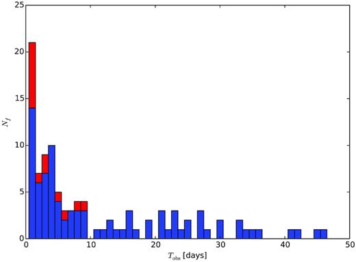
Number of fields Nf with observation time per field Tobs for the ASKAP/CRAFT ‘lat50’ survey reported in Shannon et al. (2018). Primary fields at Galactic latitude |b| = ±50○ are shown in blue; secondary fields are shown in red.
A total of 57 primary fields were studied at |b| = ±50○, separated by 5.4○ in Galactic longitude (shown in blue). For each field, the total time observation time was spread between January 2017 and March 2018. Coverage was not uniform, since fields with high elevation angles were preferentially targeted, and observations times with antennas undergoing commissioning were opportunistic. Additionally, a small number of other fields were included in the survey. Most of these varied Galactic latitude by ±5○ to maximize overlap with the beam of the Murchison Widefield Array (Sokolowski et al. 2018), while some targeted high-latitude FRBs detected by the Parkes radio telescope. The durations of these pointings are indicated in red in Fig. 1.
3.1 ASKAP/CRAFT lat50 beamshape
The beam configuration of ASKAP for most of the survey was ‘closepack36’, with total sensitivity Ω(B) derived in James et al. (2019a). The calibration procedure resulted in uncertainties regarding the outer beam sidelobes – Ω(B) is plotted for both the ‘worst case’ (largest sidelobe) and ‘best case’ (lowest sidelobe) beamshapes in Fig. 2.
![Inverse beamshapes Ω(B) for the closepack36 beam configuration. Best and worst-case sidelobes correspond to different assumptions made during beam calibration [see James et al. (2019a) for details]. ‘Truncated 1d’ results are calculated by first setting beamshapes B(Ω) to zero when fields overlap in Galactic longitude (i.e. in one dimension of the beamshape).](https://oup.silverchair-cdn.com/oup/backfile/Content_public/Journal/mnras/486/4/10.1093_mnras_stz1224/1/m_stz1224fig2.jpeg?Expires=1750189791&Signature=nCoj8aBewGelQNYFPRsa4bCGf71nqDhVli9pI3DJm2rT1X2wki1ceEoOq8oEpXkEVYvZZ9FEonp8Qj~fxDgeb8GimjBoAgbyHSWxWwnJWZLRS2tPuY9OUizd3oQblx1q8tBSX~SIU6fkK9iLZEgGXqWoW5o~EcWkH8Z6l6-dExj8UB8b6MNy0N3z2cNjM~n9tBHiDlXSPKfaWbpsYtXLpmEK1S-aTpTkK0p~wEUx-K6Qt22Et29qzPZhLSbNnPmyo6YF590PKNl36AtjVPX0ab9dDsm68eypc4pA2L3IykmySaH1ZSbPSlKuGNX-PjL4kFQRW4CjnBpI9a8j6dm5DA__&Key-Pair-Id=APKAIE5G5CRDK6RD3PGA)
Inverse beamshapes Ω(B) for the closepack36 beam configuration. Best and worst-case sidelobes correspond to different assumptions made during beam calibration [see James et al. (2019a) for details]. ‘Truncated 1d’ results are calculated by first setting beamshapes B(Ω) to zero when fields overlap in Galactic longitude (i.e. in one dimension of the beamshape).
Following the procedure suggested in Section 2.5, Ω(B) is also calculated by truncating the beams in the direction of Galactic longitude (i.e. one dimension), where adjacent fields overlapped.
For all beamshapes, the peak in the range −0.3 < log10(B) < 0 represents the solid angle spanned by the 36 ASKAP beams near FWHM, while Ω(B) for lower beam power B is the solid angle spanned by sidelobes. The downturns below log10(B) < −2 for the worst-case beams is artificial, and due to the beamshapes being calculated over an 8○ × 8○ region only.2
Since the goal of this work is to calculate upper limits from the non-observation of repeat pulses, from now on only the best-case sidelobes are considered, which (despite the nomenclature) will produce the worst limits on the presence of FRBs through lower total sky coverage.
3.2 ASKAP/CRAFT lat50 sensitivity
The expected total DM of an FRB can be calculated as per Inoue (2004); here, a fully ionized, uniform intergalactic medium with an electron number density in the current epoch of ne(z = 0) = 9.898 × 10⁻⁶Ωbh2 and physical baryon density Ωbh2 = 0.02264 (Bennett et al. 2013) is assumed. No inhomogeneities (see e.g. McQuinn 2014) are considered. Doing so (i.e. ignoring inhomogeneities) produces an approximate intergalactic DM contribution DMIGM of 100 pc cm−3 at z = 0.1 and 1100 pc cm−3 at z = 1, to which would be added Galactic and host contributions, and the DM from intervening galaxies and haloes. For this sample, the total Galactic contribution from the NE2001 model of Cordes & Lazio (2002) is less than 65 pc cm−3, assuming a Galactic halo contribution of 15 pc cm−3 as per Shannon et al. (2018). Thus, at z = 1 the minimum dispersion smearing of a pulse would smear it over four samples. Rather than use a z-dependent threshold therefore, the ASKAP fluence threshold F0 is set at twice the nominal value, i.e. F0 = 52 Jy ms, to account for burst smearing over four samples. A z-dependent threshold is considered in Section 6.
Using this threshold, and noting that zcrit ≈ 0.19 for ASKAP, Fig. 3 shows zlim corresponding to different values of beam sensitivity B (and hence threshold Fth) as a function of observation time Tobs. The most sensitive observations (B = 1 and Tobs ∼ 50 days) produce zlim = 0.7 (DMIGM = 770 pc cm−3) at 68 per cent CL. This range of zlim is broadly consistent with the assumed threshold, which will only be too optimistic for FRBs near z = 0.7 with significant host or halo contributions, and too pessimistic for FRBs at low z (corresponding to zlim for low B, Tobs, and 95 per cent CL) with little to no host or halo contribution.
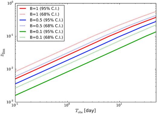
Dependence of zlim on observation time Tobs at different beam sensitivities B and confidence levels CL for an ASKAP threshold of F0 = 52 Jy ms, assuming a Poissonian distribution of burst arrival times.
Fig. 4 plots Ω(zlim) for the ASKAP/CRAFT lat50 survey, calculated as per equation (12). The structure in the range −2.0 < log10(zlim) < −0.9 mimics that of the pointing time histogram. In the truncated case, the removal of sidelobes in one dimension becomes increasingly important at low redshifts. Ω(zlim) is likely underestimated for log10(zlim) ≤ −2.5, since in this region, far sidelobes – which are not included in the ASKAP beamshape estimates – will become important.

The region of sky Ωlim(z) (equation 13) over which the presence of an FRB can be limited is shown in Fig. 5, for the best-case, truncated beam only (see Section 2.5). At low values of z, the total solid angle covered converges on 2 sr. This is approximately double the survey area that would be calculated using the nominal field of view of ∼30 deg2 and the total number of survey fields (Nf = 103), and is due to the influence of sidelobes. Note that the value of Ωlim(z) as z → 0 is somewhat arbitrary, since any radio telescope will cover all 2|$\pi$| sr of the sky at some non-zero value of B. In this case, Ωlim(z) is only greater than the nominal survey area for log10(z) ≲ −2.0 at 95 per cent CL.

The influence of low-sensitivity sidelobes on final limits on repetition is shown to be negligible in Fig. 6, which plots the integrand of equation (14). That is, it is a volume-weighted version of the Ωlim(z) shown in Fig. 5. The much greater volume probed at high z results in a very strong dependence on beam sensitivity, reducing the influence of sidelobes. It also means that the chosen level of confidence has a large effect on the resulting volumetric limits.
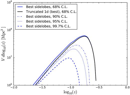
Volumetric limit as a function of z within which the presence of an FRB can be excluded at the stated CLs. Standard results are for the best-case sidelobes; the truncated beam at |$68{{\ \rm per\ cent}}$| CL is presented for comparison purposes only. Calculations correspond to the integrand of equation (14). Assumed FRB properties are given by equations (1) and (2) with Poissonian arrival times.
Integrating over the limited volume of Fig. 6 as per equation (14) produces volumetric limits shown in Table 1. At 95 per cent CL, the presence of a repeating FRB with burst energy distribution given by equations (1) and (2) with Poissonian arrival times can be excluded in a volume of 8.4 × 10⁶ Mpc3. However, the burst arrival time distribution of FRB 121102 is clearly non-Poissonian – this is investigated in the next section.
| CL (per cent) | Vlim (Mpc3) |
|---|---|
| 68 | 2.6 × 10⁷ |
| 90 | 1.2 × 10⁷ |
| 95 | 8.4 × 10⁶ |
| 99.7 | 3.8 × 10⁶ |
| CL (per cent) | Vlim (Mpc3) |
|---|---|
| 68 | 2.6 × 10⁷ |
| 90 | 1.2 × 10⁷ |
| 95 | 8.4 × 10⁶ |
| 99.7 | 3.8 × 10⁶ |
| CL (per cent) | Vlim (Mpc3) |
|---|---|
| 68 | 2.6 × 10⁷ |
| 90 | 1.2 × 10⁷ |
| 95 | 8.4 × 10⁶ |
| 99.7 | 3.8 × 10⁶ |
| CL (per cent) | Vlim (Mpc3) |
|---|---|
| 68 | 2.6 × 10⁷ |
| 90 | 1.2 × 10⁷ |
| 95 | 8.4 × 10⁶ |
| 99.7 | 3.8 × 10⁶ |
4 BURST TIME DISTRIBUTION
The method of Section 2 can be adapted to any time-distribution of bursts, provided that the probability of observing two or more events in the observation period is a readily calculable function of the expected number of events, λ. This then allows λlim to be set to the value at which this probability is equal to the desired level of confidence.
The time distribution of bursts from FRB 121102 is clearly non-Poissonian – this object either has ‘active’ and ‘inactive’ modes, or a ‘bursty’ distribution, over a variety of time-scales (Law et al. 2017; Gajjar et al. 2018; Zhang et al. 2018).3 Connor, Pen & Oppermann (2016) provide a general discussion of non-Poissonian statistics in the context of FRB observations.
Oppermann, Yu & Pen (2018) modelled the distribution of burst arrival times of FRB 121102 as a Weibull distribution. Their fit used data from Spitler et al. (2016) and Scholz et al. (2016), with single observations lasting of order 1 h, and spanning the period from late 2011 to early 2016 (over 3 yr). The fitted index (or shape parameter) k of the Weibull distribution was |$k=0.34^{+0.06}_{-0.05}$| with mean rate |$R=5.7^{+3.0}_{-2.0}$| day−1. A value of k = 1 replicates a Poissonian distribution, and k < 1 implies data which is more clustered, resulting in a greater probability to see both zero and many events. Limiting the presence of a repeating FRB with burst arrival times following a Weibull distribution with k < 1 therefore requires increasing λlim in comparison to Poissonian values.
The probabilities of viewing a given number of events in the case of a single continuous pointing are derived in Oppermann et al. (2018). In particular, the probability of viewing zero or one events – and hence the probability of viewing two or more – is readily evaluated. The resulting values of λlim required for a given level of confidence are shown in Table 2 (columns 2–4). For observations spanning multiple pointings, no analytic expression is obtainable, and the exact case must be simulated through Monte Carlo methods. It is also impossible to reduce multiple overlapping pointings to a single effective exposure (see Section 2.5), as is the case for a Poissonian distribution. In the limit of many short pointings separated by large intervals, however, the expected rate will again become Poissonian.
Critical expectation values, λlim, corresponding to different CLs in three cases of burst time distributions: a Poissonian distribution; a Weibull distribution with shape parameter k viewed by a continuous pointing; and a Weibull distribution viewed by a typical time distribution of CRAFT lat50 pointings.
| λlim | |||||||
|---|---|---|---|---|---|---|---|
| Poisson | Single continuous pointing | CRAFT lat50 pointing | |||||
| CL (per cent) | (k = 1) | k = 0.29 | k = 0.34 | k = 0.40 | k = 0.29 | k = 0.34 | k = 0.40 |
| 68 | 2.36 | 12.5 | 8.08 | 5.7 | 4.6 | 3.8 | 3.2 |
| 90 | 3.89 | 45.0 | 25.4 | 15.8 | 12.3 | 8.6 | 6.6 |
| 95 | 4.84 | 76.5 | 40.8 | 23.9 | 18.4 | 11.9 | 8.7 |
| 99.7 | 7.83 | 330 | 150 | 75.2 | 57 | 30 | 20 |
4.1 λlim for the CRAFT lat50 survey
The CRAFT lat50 survey is an intermediate case of observations spanning typically a few hour per pointing, and totalling several tens of days per survey field, over a 1-yr period. A full calculation of the requisite probabilities of detecting a repeating FRB with burst times following a Weibull distribution therefore would require a dedicated calculation for each and every pointing. To make this tractable, this calculation is performed for a single field only, ‘G217-50’, centred at Galactic coordinates l = 217○, b = −50○. This field was observed for the greatest duration (45.3 antenna-days after accounting for efficiency losses), with observations spread over 172 periods, averaging 6.3 h each. This field is chosen not only because it has the greatest impact on the volumetric limit, but also because fields with shorter total pointing duration could either more sparsely span the same time period, and thus have a more Poissonian distribution of burst probabilities (and hence lower λlim); or be observed with equal regularity, but span a shorter period, and thus tend more towards the single continuous pointing case (and hence higher λlim).
In order to simulate the detection probabilities for a Weibull distribution of burst times in terms of k and R, care must be taken that R is specified in terms of true days, not days observed. A random series of burst waiting times, and hence burst actual times, is then generated, setting the first event to be much earlier than the first observation. The full series is then generated over the observation period, and bursts occurring during the observation times count as being detected. This process is then repeated 104 times for each combination of (k, R) in order to estimate the probability of detecting any given number of events n, allowing the value of R, Rlim, corresponding to a given confidence limit to be obtained. λlim can then be calculated by multiplying Rlim by the total observation time Tobs. These values are shown in Table 2. While the effects of clustering still act to require a higher number of expected events before the presence of an FRB can be excluded at a given CL, the required values are much lower than in the case of a single continuous pointing.
Using these modified values of λlim for k = 0.34, and repeating the calculations of Section 3, produces limiting solid angles Ωlim(z) given in Fig. 7. As expected, Ωlim(z) is contracted to smaller values of z when compared to the Poissonian case (Fig. 4). The resulting values of Vlim, after applying equation (14), are given in Table 3 (second column).

Solid angle Ωlim(z) over which the presence of a repeating FRB with properties given by equations (1) and (2) can be excluded as a function of z at the stated CLs, assuming a Weibull distribution of burst arrival times with shape parameter k = 0.34. Calculations use truncated beams with best-case sidelobes.
Values of Vlim (Mpc3) for repeating FRBs over the range of parameter values compatible with FRB 121102. The units of R0 are day−1.
| CL (per cent) | R0 = 7.4, γ = −0.9, k = 0.34 | R0 = 2.6 | R0 = 11.4 | γ = −0.7 | γ = −1.1 | k = 0.29 | k = 0.40 |
|---|---|---|---|---|---|---|---|
| 68 | 1.2 × 10⁷ | 1.7 × 10⁶ | 1.9 × 10⁷ | 4.8 × 10⁷ | 3.2 × 10⁶ | 7.2 × 10⁷ | 1.3 × 10⁷ |
| 90 | 3.3 × 10⁶ | 4.2 × 10⁵ | 5.2 × 10⁶ | 1.0 × 10⁷ | 9.9 × 10⁵ | 1.4 × 10⁶ | 4.3 × 10⁶ |
| 95 | 1.9 × 10⁶ | 2.4 × 10⁵ | 3.1 × 10⁶ | 5.4 × 10⁶ | 6.2 × 10⁵ | 6.9 × 10⁵ | 2.6 × 10⁶ |
| 99.7 | 3.8 × 10⁵ | 4.9 × 10⁴ | 6.2 × 10⁵ | 7.4 × 10⁵ | 1.7 × 10⁵ | 9.8 × 10⁴ | 6.3 × 10⁵ |
5 VARYING PROPERTIES OF THE REPEATER
The properties of FRB 121102 are hardly well constrained, and furthermore, it would be astounding if all repeating FRBs in the Universe repeated with identical properties to that of FRB 121102. The simplest variation is to consider other values of the standard parameters of equation (2). Given that R0 and E0 are degenerate, E0 is kept constant, and the analysis of Section 4 is repeated for different values of R0 and γ, and the shape parameter of the Weibull distribution, k. In each case, other values of the parameters are fixed to their standard values, i.e. |$R_0=7.4\, {\rm day}^{-1}$|, γ = −0.9, and k = 0.34.
Fig. 8 shows the 95 per cent CL upper limits on Vlim resulting from varying γ in the range −0.5 to −1.5; Fig. 9 does the same when varying R0 (the rate above 1.7 · 1038 erg) between 0.074 and 740 day-1; while Fig. 10 varies k between 0.1 and 1.0 (i.e. a Poisson distribution). Specific values of Vlim for the ranges of R0, γ, and k consistent with FRB 121102 are given in Table 3.


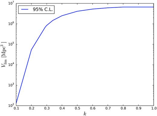
Dependence of Vlim on the Weibull shape parameter k from equation (1), holding other parameters constant. Note that k = 1.0 corresponds to a Poisson distribution of burst arrival times.
Since γ determines the trade-off between sensitivity and observing time (i.e. how much longer one has to wait to view very bright events), steeper (more negative) values of γ reduce the ability of the long ASKAP/CRAFT pointings to probe large volumes of the distant universe using rare, very bright pulses. However, they do not greatly reduce the ability of short observations to observe regular weak pulses from repeating FRBs in the local Universe. The variation in Vlim for −1.5 < γ < −0.5 none the less covers two orders of magnitude.
The dependence of limiting volume on R0 is very strong. Since γ is almost unity, reducing the intrinsic rate by an order of magnitude requires a reduction in observable intrinsic burst energy of almost the same factor through equation (1). This then reduces zlim almost with the square root of R0, and hence Vlim varies approximately as |$R_0^{1.5}$|, which is clearly observed in Fig. 9. The reduction in slope for large R is due to the universe at z > 1 being probed, where cosmological effects become important.
Finally, as k is reduced from the Poissonian value of 1, burst arrival times become more clustered. This increases both the probability of seeing zero and many events at the expense of viewing a few. For values of 0.8 ≤ k ≤ 1, the timing of the observations results in estimated values of λlim, and hence Vlim, being identical to within simulation accuracy of the Poissonian case (k = 1). However, as k becomes small, very large values of λlim are required to exclude the possibility of viewing no repeat events. For example, for k = 0.1 at |$95{{\ \rm per\ cent}}$| CL, λlim ∼ 2900, and only a tiny local volume of 100 Mpc3 is probed. Since the probability of viewing a single event becomes negligible in the case of low values of k, this suggests that the best limits on very bursty FRBs will be derived from the observation of single bursts, rather than the non-observation of repeating bursts as performed here.
6 LIMITS ON THE POPULATION DENSITY OF REPEATING FRBS
The simple method above ignores that limits will be more stringent when considering larger volumes over which the detection probability of individual repeating FRBs is smaller. Furthermore, it cannot account for changing population densities with redshift, i.e. Φ → Φ(z).
6.1 Volumetric limits from the ASKAP/CRAFT lat50 survey
In order to limit Φ0, the z-dependence of the FRB population density ϕ(z) is chosen to be an integer power n of the star formation rate (SFR). As per Macquart & Ekers (2018b), values of n = 0 (no dependence), n = 1 (stellar origin), and n = 2 (approximately tracing AGN activity) are considered. Evidently, this does not encompass models with significant delay-time, e.g. long-duration mergers, as tested by Cao, Yu & Zhou (2018).
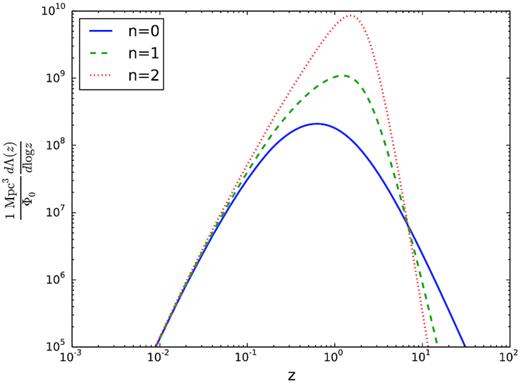
Expected rate of detection λ(z) of repeating FRBs similar to FRB 121102 as a function of redshift z, for the standard parameter set R0 = 7.4 day −1, γ = −0.9, k = 0.34. The normalized FRB population density ϕ(z) is assumed constant (n = 0; solid), or scales as the SFR to the power of n = 1 (dotted) and n = 2 (flat).
For n = 0, the distribution peaks near z = 0.6, rising to z = 1.2 for n = 1 and z = 1.5 for n = 2. Furthermore, while using a clustered burst time distribution (k < 1) increases the chance of seeing no events when the expected rate is high (i.e. in the near universe), it also increases the chance of seeing two or more events when the expected rate is low (i.e. in the distant universe). The first effect reduces the volume in which the presence of a single FRB can be excluded with high confidence, as shown in Section 4. However, when considering the total detection rate of repeating FRBs, the second effect actually increases the expected number. This is because the dominant contribution arises from the larger population at high redshift, where the expected number of bursts λ for a given FRB is small, and the probability of observing two or more bursts increases as k decreases.
However, the high redshifts probed in Fig. 11 illustrate a deficit in the chosen burst energy distribution given in equation (1): there is no maximum burst energy. Shannon et al. (2018) finds maximum FRB energies near 1033 erg Hz−1 (1042 erg assuming a 1 GHz emission bandwidth), while Luo et al. (2018) find maximum burst energies of 2 × 1044 erg s−1 (2 × 1041 erg assuming a 1 ms duration). A two-population scenario where repeating FRBs are only responsible for the weaker observed bursts will result in even lower energy cut-offs.
Recalculating the limits produces Fig. 12, with corresponding 95 per cent upper limits on the population density (i.e. Λrep = 4.84 in equation 22) given in Table 4. Values of Ecut between 1040 erg (where pulses from FRB 121102 have been observed Law et al. 2017) and 1043 erg (well above all known pulse strengths, and beyond which values take their infinite limits) were considered. The result at 1042 erg is taken to be the ‘nominal’ value, i.e. consistent with all FRBs being due to repeaters similar to FRB 121102.

Differential rate of detection of repeating FRBs similar to FRB 121102 as a function of redshift z, for the standard parameter set R0 = 7.4 day −1, γ = −0.9, k = 0.34, normalized by Φ0. Different colours assume different maximum FRB burst energies Ecut (see labels). The normalized FRB population density ϕ(z) is assumed constant (n = 0; solid), or scales as the SFR to the power of n = 1 (dotted) and n = 2 (flat).
Upper limits at 95 per cent CL on Φ0 (repeating FRBs per Gpc3 in the current epoch) for different assumptions about the maximum burst energy Ecut and population evolution (scaling with the SFR to the power n).
| Ecut (erg) | n = 0 | n = 1 | n = 2 |
|---|---|---|---|
| 1040 | 540 | 450 | 380 |
| 1041 | 82 | 54 | 34 |
| 1042 | 27 | 12 | 4.8 |
| 1043 | 15 | 4.7 | 1.1 |
| None | 12 | 3.0 | 0.55 |
| Ecut (erg) | n = 0 | n = 1 | n = 2 |
|---|---|---|---|
| 1040 | 540 | 450 | 380 |
| 1041 | 82 | 54 | 34 |
| 1042 | 27 | 12 | 4.8 |
| 1043 | 15 | 4.7 | 1.1 |
| None | 12 | 3.0 | 0.55 |
As expected, the effect of a strong dependence on SFR increases for high values of Ecut, since this allows the more-distant universe to be probed. For Ecut = 1042 erg – close to the derived value for all FRBs – limits vary by a factor of 2 for each successive n, suggesting that ASKAP observations of repeating FRBs could limit the population evolution model.
Fixing Ecut = 1042 erg, and varying R0, γ, and k over the uncertainties of FRB 121102, produces limits on the number of repeating FRBs per Gpc3 in Table 5. Unlike the case of excluding the presence of an FRB in a certain volume Vlim, where changes in the same range of parameters vary the resulting excluded volumes over three orders of magnitude (see Table 3), limits on Φ0 vary by only a single order of magnitude over the same range of parameters. One key difference is that varying the Weibull shape parameter k only weakly affects these limits – indeed, limits become stronger for k < 1, although they again become weaker for k < 0.34. A steeper burst energy distribution (γ = −1.1) and an intrinsically lower rate (R0 = 2.6 day −1) result in the weakest limits, at Φ0 < 70 FRBs Gpc−3.
Upper limits at 95 per cent CL on Φ0 (repeating FRBs per Gpc3 in the current epoch) for different assumptions about FRB parameters R0, γ, and k, as a function of the population evolution scaling parameter n). The energy cutoff Ecut is fixed to 1042 erg. The standard scenario uses R0 = 7.4 day −1, γ = −0.9, k = 0.34.
| n | Standard | R0 = 2.6 | R0 = 11.4 | γ = −0.7 | γ = −1.1 | k = 0.29 | k = 0.40 | k = 1 |
|---|---|---|---|---|---|---|---|---|
| 0 | 27 | 68 | 19 | 11 | 70 | 29 | 26 | 34 |
| 1 | 12 | 33 | 8.2 | 4.8 | 35 | 13 | 12 | 19 |
| 2 | 4.8 | 14 | 3.2 | 1.9 | 15 | 4.9 | 4.9 | 9.7 |
| n | Standard | R0 = 2.6 | R0 = 11.4 | γ = −0.7 | γ = −1.1 | k = 0.29 | k = 0.40 | k = 1 |
|---|---|---|---|---|---|---|---|---|
| 0 | 27 | 68 | 19 | 11 | 70 | 29 | 26 | 34 |
| 1 | 12 | 33 | 8.2 | 4.8 | 35 | 13 | 12 | 19 |
| 2 | 4.8 | 14 | 3.2 | 1.9 | 15 | 4.9 | 4.9 | 9.7 |
This highlights that while the detection of multiple pulses from any specific repeating FRB in a volume of the universe is both far from likely and highly dependent on particular FRB parameters, the chance of detecting multiple pulses from any repeating FRB at much farther distances is much higher, and more robust to changes in FRB parameters.
6.2 Comparison to the singles rate
This work has so far concentrated on repeat bursts only, the motivation being that single bursts can be explained by a much wider space of FRB parameters. The ASKAP/CRAFT lat50 survey detected 20 single bursts, 19 of which were above the nominal detection threshold of |$9.5\, \sigma$| (Shannon et al. 2018), which begs the question – can these 19 events arise from the allowed population of repeating FRBs?
Until now, all limits on repeating FRBs have been calculated conservatively, i.e. using lowest sidelobe beamshapes, setting the telescope threshold according to the DM smearing from objects at high z, and ignoring the effects of sidelobes on overlapping survey fields. However, placing the most conservative limit on repeating FRBs may correspond to an upper, lower, or intermediate limit on the expected ratio of single to multiple pulses.
Of the effects noted above, using large (worst-case) sidelobes increases the total sensitivity of the telescope to FRB bursts, but without high sensitivity in any given direction, thus favouring single bursts. Since much of this sensitivity will be in neighbouring survey fields, in reality this will help to discover repeat bursts. However, ignoring this effect – as per the discussion of Section 2.5 – will mean only increased sensitivity to single bursts will be accounted-for.
Using a redshift-dependent threshold may or may not favour single versus multiple bursts, warranting the extra complexity of modelling it. Therefore, the full z-dependent threshold of equation (19) is used, using the treatment of Section 3.2. The resulting threshold F0(z) is given in Fig. 13. While this ignores significant contributions from host galaxies and intervening large-scale structures, and breaks down when the IGM ceases to be fully ionized, it should adequately reflect the changing sensitivity to the majority of FRBs in the z < 1 range. This z-dependent threshold then affects the calculation of the expected number of observed bursts in equation (22).
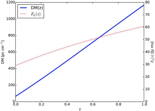
Modelled dependence of DM, and hence detection threshold F0, on redshift z.
Keeping Ecut = 1042 erg (since any lower value cannot by definition account for all singly observed bursts), Λ1 is evaluated for the range of repeating FRB parameters investigated in Table 5.
Calculations used both best-case and worst-case beamshapes. However, the results differed by less than 1 per cent throughout the entire parameter space, and in Table 6 and from hereon, results for best-case beamshapes only are shown.
Maximum expected number of single FRB bursts, Λ1, from the ASKAP/CRAFT lat50 survey, assuming a population of repeating FRBs equal to the 95 per cent CL upper limits – and corresponding parameters – from Table 5.
| n | Standard | R0 = 2.6 | R0 = 11.4 | γ = −0.7 | γ = −1.1 | k = 0.29 | k = 0.40 | k = 1 |
|---|---|---|---|---|---|---|---|---|
| 0 | 3.4 | 4.8 | 2.9 | 2.3 | 4.5 | 2.5 | 4.4 | 14 |
| 1 | 4.0 | 5.7 | 3.5 | 2.6 | 5.5 | 3.0 | 5.3 | 18 |
| 2 | 4.7 | 6.7 | 4.0 | 3.0 | 6.7 | 3.5 | 6.3 | 24 |
| n | Standard | R0 = 2.6 | R0 = 11.4 | γ = −0.7 | γ = −1.1 | k = 0.29 | k = 0.40 | k = 1 |
|---|---|---|---|---|---|---|---|---|
| 0 | 3.4 | 4.8 | 2.9 | 2.3 | 4.5 | 2.5 | 4.4 | 14 |
| 1 | 4.0 | 5.7 | 3.5 | 2.6 | 5.5 | 3.0 | 5.3 | 18 |
| 2 | 4.7 | 6.7 | 4.0 | 3.0 | 6.7 | 3.5 | 6.3 | 24 |
The effect of a z-dependent threshold acted to increase the sensitivity to repeat bursts in comparison to single bursts, i.e. the limits in Table 6 are weaker by typically tens of per cent when using an (incorrect) constant threshold.
Except for repeating FRBs with Poissonian (k = 1) arrival times, none of the parameter combinations examined in Table 6 can produce the 19 single burst events seen by the ASKAP/CRAFT lat50 survey within the limits set in Section 6.1. However, the allowed number of single bursts is only a factor of a few below that observed, and could likely be explained by a larger population of repeating FRBs having a lower rate, or less bursty arrival times. While the ratio of single to multiple bursts also increases with increasing (less negative) γ, extremely flat burst energy distributions (γ → 0) seem implausible.
At what rates R0 are the expected number of single bursts Λ1 consistent with limits on the population density, Φlim, and the observed value of 19? In the case of Poissonian arrival times, this is already almost consistent for R0 = 7.4 day −1. The case of k = 0.34 is shown in Fig. 14 – only a population of repeaters with R0 ≤ 0.02 day −1 are consistent at 95 per cent CL. This suggests that either the majority of repeaters are less bursty, or repeat less often, than FRB 121102.
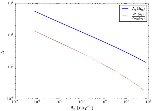
Expected number of single bursts Λ1 as a function of repetition rate, R0, for (blue solid line) a population consisting entirely of FRBs with rate R0; and (red dotted line) the differential rate of single bursts from a population consisting of the distribution in R0 from equation (30). In the latter case, the integral equates to 18 single bursts.
6.3 Comparison to the observed DM/redshift distribution
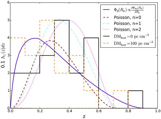
It is also relevant to compare the redshift distribution of observed ASKAP/CRAFT lat50 FRBs with that predicted from the integrand of equation (29). This is shown in Fig. 15, for four cases of R0, and standard parameters k = 0.34, γ = −0.9, Ecut = 1042 erg, and n = 0. The redshifts of ASKAP/CRAFT lat50 FRBs are calculated from the observed DMs (Shannon et al. 2018), and assuming a total Galactic (including halo) contribution of 65 pc cm−3 as per Section 3.2. Host galaxy contributions, DMhost, were set at 0 and 100 pc cm−3 (histograms). The DMhost = 0 case is not consistent with any rate: either the total number of single bursts is underpredicted (R0 = 0.74 and 7.4 day −1), or the peak of the redshift distribution is too low (R0 = 0.074 and 0.0074 day −1). Assuming DMhost = 100 is generally consistent in both shape and magnitude with the R0 = 0.074 and 0.0074 day −1 cases.
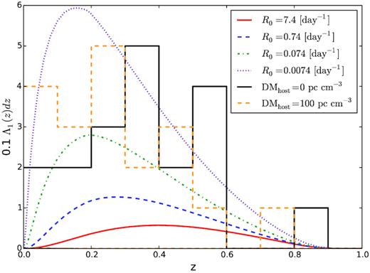
Expected number of single bursts Λ1 in the ASKAP/CRAFT lat50 survey as a function of redshift for populations of identical repeating FRBs producing Λrep = 4.84 repeating sources. Four values of R0 are considered; all other parameters are held constant at k = 0.34, γ = −0.9, Ecut = 1042 erg, and n = 0. Also, plotted are redshift histograms from the ASKAP/CRAFT lat50 survey for 19 above-threshold FRBs, calculated from observed DMs assuming no host DM contribution (black histogram) and a contribution of DMhost = 0 pc cm−3 (orange histogram).
Expected number of single bursts Λ1 in the ASKAP/CRAFT lat50 survey as a function of redshift for different repeating FRBs populations. Three cases where all FRBs are identical are considered, with Poissonian burst arrival times (k = 1), γ = −0.9, and Ecut = 1042 erg; only the scaling parameter n of the population density with the SFR is varied. A fourth case, being the population of repeating FRBs with R0 distribution described by equation (31), and k = 0.34, γ = −0.9, Ecut = 1042 erg, and n = 0 is also shown. In the n = 1 and n = 2 cases, the distribution is normalized to 19 single bursts; in the other two cases, no normalization is applied. Also, plotted are redshift histograms from the ASKAP/CRAFT lat50 survey for 19 above-threshold FRBs, calculated from observed DMs assuming no host DM contribution (black histogram) and a contribution of DMhost = 0 pc cm−3 (orange histogram).
An alternative is that the majority of FRBs obey Poisson statistics, also shown in Fig. 16. The observation of an FRB at z > 0.8 is unlikely in this model, ruling out agreement with DMhost = 0, while too few low-z bursts are predicted when DMhost = 100. Changing the dependence on the SFR from n = 0 to n = 1 or n = 2 (also shown) allows more single bursts than observed. Since a population density less than the maximum allowed by the 95 per cent CL limit (Λrep = 4.84) is clearly possible, the predicted number of single bursts have been re-scaled to the observed number of 19. Doing so only slightly shifts the distribution to the right, however, and solves neither problem.
Further modelling of the full FRB population, including more sophisticated models of DM, and explicit fits to data, is left to a future work.
7 DISCUSSION
The primary result of this work is that the non-observation of repeating pulses in the ASKAP/CRAFT lat50 survey excludes the presence of any repeating FRBs with properties similar to that of FRB 121102 in a volume of 1.9 × 10⁶ Mpc3 at 95 per cent CL. The volume over which FRBs can be excluded ranges from 2.4 × 10⁵ Mpc3 when considering FRBs repeating at the lowest rate estimates for FRB 121102 (R0 = 2.6 day −1), to 5.4 × 10⁶ Mpc3 when considering FRBs with a flatter distribution of pulse strengths (γ = −0.7). The limited volume increases to 8.4 × 10⁶ Mpc3 in the case of a Poissonian distribution of burst arrival times. These ranges are not uncertainties in the limited volume – they are uncertainties in the properties of FRB 121102. Rather, the greatest uncertainties in these limits are due to uncertainties in the ASKAP beamshape, and the treatment of overlapping beamshapes from neighbouring fields. The treatment chosen here is always the most conservative, and a more complete treatment could only act to strengthen the limits. Thus, the limits derived here are robust.
The properties of any purported repeating FRB strongly affect the volume over which it can be limited. For instance, extremely bursty FRBs with burst times following a Weibull distribution with shape parameter k = 0.1 can only be excluded in a volume of 100 Mpc3 at 95 per cent CL. Conversely, limits on extremely bright FRBs are very strong: no FRBs with a rate of 1000 day −1 exist within a volume if 1 Gpc3 (95 per cent CL). Importantly, limits apply independently at each part of the parameter space, e.g. both limits for k = 0.1 and R0 = 1000 day −1 apply simultaneously and independently. For practical reasons, limits for only a small range of parameter combinations have been presented here.
Limiting the population of repeating FRBs as a whole becomes sensitive to any high-energy cut-off in the burst rate, and the population evolution with redshift. Of the range of scenarios covered by Table 4, there are two ‘benchmark’ cut-offs, Ecut. These are Ecut = 1040 erg, which is consistent with the burst energies observed from FRB 121102, but requires a separate population to explain non-repeating bursts; and Ecut = 1042 erg, which covers all known FRBs. Respective upper limits at 95 per cent CL on the population density Φ0 at z = 0 are very low, at 540 FRBs Gpc−3 and 27 FRBs Gpc−3. They are stronger for any evolutionary scenario.
That the number of above-threshold single bursts (19) observed in the ASKAP/CRAFT lat50 survey cannot be explained by repeating populations of FRBs within these limits indicates a population of less frequently repeating FRBs; FRBs repeating with Poisson statistics; or a second population of once-off bursting objects. Compared with the observed DM (∼redshift) distribution, the only consistent scenarios found were a population of FRBs producing no more than 0.074 bursts day−1 above 1.7 × 1038 erg, or a population with a distribution of rates of |${\rm d}\Phi /{\rm d}R_0 \propto R_0^{-2.1}$|. These both required DM contributions from host galaxies to fit the observed distribution. Populations of repeating FRBs obeying Poisson statistics were less consistent, while invoking an appropriate second population of once-off bursts would also have reproduced observations. What can be ruled out with very high confidence is that FRB 121102 is not a typical FRB: it repeats when most do not; it repeats much more frequently than is typical; or (less likely) it repeats with much burstier statistics than is typical.
The only comparable study of the population density of repeating FRBs is that by Caleb et al. (2019). These authors use burst indices in the range 0 > γ > −1 over the burst energy range of 1035–1043 erg, a broad range of intrinsic rates, a population evolving with the SFR (n = 1), and both Weibull and Poisson distributions. A Monte Carlo simulation is used, allowing the DM to be modelled in much greater detail than is performed here. Caleb et al. (2019) do not model a particular survey; however, a single instance of their simulation for a population of Poissonian-distributed FRBs produces 15 single bursts and 3 repeating sources in a hypothetical all-sky survey with Parkes. The true expectation values for single and multiple bursts will thus be in the range |$15^{+5}_{-3}$| and |$3_{-0.9}^{+2.9}$|, respectively (68 per cent confidence intervals). This is similar to the ratios found here, although the difference in beamshape and total time per pointing make exact comparisons difficult. Caleb et al. (2019) also claim that the chance of ASKAP observing repeat pulses is ‘highly unlikely’. This claim is clearly contradicted, since the non-observation of repeat bursts is shown here to be significant, and constrains the population distribution of repeating FRBs.
7.1 Notes of caution
There are three mains caveats to these limits. First, all limits presented in this work apply only in the case of isotropic emission. If, as seems likely, FRBs are beamed with beaming factor fb (i.e. into an angle of 4|$\pi$|/fb sr), then the limits do not apply to FRBs with emission beamed away from Earth, and they will be a factor of fb weaker. This assumes a constant beaming direction for all bursts from a given FRB. If the beaming direction is varies burst to burst, then the rate R should be interpreted as the observed burst rate, with the true burst rate being higher. In such a case, the nominal rate of R0 = 7.4 day −1 for FRB 121102 is also the observed rate, and the limits therefore do not change. Such a consideration does not apply however to conclusions derived from the ratio of single to multiple bursts.
Secondly, no frequency dependence of the FRB rate or spectrum is considered, although the methods clearly could be adapted to such a consideration. The ASKAP/CRAFT lat50 survey from which these limits derive covered the frequency range of 1128–1464 MHz, with observed FRBs found to have a burst spectral index, α (fluence Fν ∝ να), of |$\alpha =-1.5^{+0.2}_{-0.3}$| (Macquart et al. 2019). Most observations of FRB 121102 (see the Appendex), however, have been at higher frequencies. If single ASKAP/CRAFT bursts are attributable to repeating FRBs observed only once (e.g. the scenarios examined in Section 6), this suggests that the lower frequency of the ASKAP/CRAFT lat50 survey was relatively more sensitive to repeating FRBs, not less. This, and the observation of FRB 180814.J0422+73 at even lower frequencies of 400–800 MHz (CHIME/FRB Collaboration et al. 2019a,b), suggests that it is unlikely that the frequency range used in this work weakens the derived limits.
It is also known that many bursts – both from FRB 121102, FRB 180814.J0422 + 73, and the single bursts detected by ASKAP/CRAFT – have complex frequency structure. If bursts occupy a narrow frequency range, which varies from burst to burst, then R0 should be interpreted as the rate at which bursts are produced between 1128(1 + z)−1 and 1464(1 + z)−1 MHz, for bursts emitted at redshift z. In this case, the fitted burst spectral index of |$\alpha =-1.5^{+0.2}_{-0.3}$| reflects not the spectral properties of the bursts themselves, but rather a higher rate of bursts at low frequencies (R ∝ να). Again, the conclusion is that bursts at low frequencies are more likely, and the limits presented here remain strong.
Thirdly, unlike Luo et al. (2018) and Caleb et al. (2018), no detailed modelling of DM contributions from FRB host galaxies or intervening structures is performed. The main effect of fully modelling the DM–z relation is to produce a small fraction of FRBs with large excess DM (McQuinn 2014; Dolag et al. 2015). By making these FRBs less detectable, the limits presented in Sections 3–5 will be slightly weakened to apply only to the majority of the FRB population. The effect is even smaller when considering the observed number of single bursts in Section 6.2, since FRBs with anonymously high DMs will not contribute to either the single or multiple burst detection probabilities. Similar considerations apply to scatter broadening, which can also lead to reduced sensitivity for a small subset of the population (Zhu, Feng & Zhang 2018).
Comparisons to the observed DM distribution in Section 6.3 must be treated with caution however – FRBs with anomalously high DMs in ASKAP/CRAFT data will produce incorrectly high redshifts. This is why models predicting too few low-z FRBs compared to data can be better excluded than those failing to predict the single high-DM (nominally 0.8 < z < 0.9) burst.
7.2 Comparison to known repeating FRBs
The two known repeating FRBs – FRB 121102 and FRB 180814.J0422+73 – are located at distances of z = 0.19273 (Chatterjee et al. 2017) and z ≲ 0.1 (CHIME/FRB Collaboration et al. 2019b), with enclosed volumes of 2.2 and 0.34 Gpc3, respectively. The limit on the population density of FRBs at z = 0 presented in Table 4 allows for at most 27 Gpc−3 in the standard scenario. This suggests that there may not be very many more nearby objects to be found. That any part of the FRB sky is even fractionally complete seems rather incongruous, given that the history of FRBs is one of a few discoveries per year against rates of thousands of bursts per sky per day. However, the advent of long-duration FRB surveys with wide field of view instruments at high sensitivity has resulted in a significant part of the sky being probed – almost 1 sr out to z = 0.03 in the case of the ASKAP/CRAFT lat50 survey. It would be interesting for limits from other FRB-hunting experiments, in particular those using Parkes and CHIME, to be calculated. All repeating FRBs in the local Universe may be discovered in the not-too-distant future.
7.3 Limits on FRB progenitor models
Several theories of FRB origin invoke object classes compatible with the long-term repetition properties of FRB 121102 (see e.g. Pen 2018; Platts et al. 2018), which has been observed to repeat since 2012 (Spitler et al. 2014). Of these models, most have no predictions for the expected FRB population density. Two cases, however – models relating to young neutron stars (NS)/magnetars (Popov & Postnov 2010; Thornton et al. 2013; Lyubarsky 2014; Pen & Connor 2015; Zhang & Zhang 2017), and magnetized white dwarfs (WDs) resulting from WD–WD mergers (Kashiyama, Ioka & Mészáros 2013) – can be estimated from the approximate population densities of their progenitor systems, allowing meaningful comparisons to limits.
The formation rate of young magnetars can be related to the rate of GRBs, since both known classes of GRB (hypernovae and compact object mergers) can lead to magnetar formation (Zhang 2014). Including sub-luminous events, the estimated rate of long-duration GRBs is 2 × 10³–2 × 10⁴ Gpc−3 yr−1 (Guetta & Della Valle 2007), while for short GRBs, it is |$1100_{-470}^{+700}$| Gpc−3 yr−1 (Coward et al. 2012). The single observed NS–NS merger also corresponds to a rate of |${\mathcal {O}}\sim 10^3$| Gpc−3 yr−1 (Abbott et al. 2017; Kruckow et al. 2018).
If a remnant magnetar (which need not be supramassive) emits repeating pulses for at least |${\mathcal {O}}\sim 10$| yr [spanning the time period over which FRB 121102 has been observed, and consistent with Yamasaki, Totani & Kiuchi (2018)], then the population density of such objects is at least 2 × 10⁴ Gpc−3. All combinations of population evolution and energy cut-off studied in Table 4 exclude this optimistic scenario at 95 per cent CL by a factor of at least 40. For Ecut = 1042 erg and n = 0, less than one in 600 such objects could produce FRBs similar to FRB 121102. Estimates of a longer emission time [e.g. Margalit et al. (2018) estimate an age of 30–100 yr for a magnetar powering FRB 121102] result in a larger population, and hence, greater conflict with these limits.
In other words, either FRB 121102 repeats much more frequently than typical objects of its class, and a large number of less frequently repeating objects abound; or only a very small fraction of GRBs produce magnetars; or a very small fraction of young magnetars produce repeating FRBs; or emission from such FRBs is strongly beamed (fb ∼ 600) and FRB 121102 is pointing towards us; or FRBs are not associated with GRBs. The first scenario is consistent with conclusions from the observed DM distribution of ASKAP/CRAFT FRBs, and by noting that the first discovered object of a population is usually exceptional (i.e. repeats more often than average; Macquart & Ekers 2018b). Integrating the population distribution of equation (31) above R0 = 0.074 day −1 produces 1750 FRBs Gpc−3, consistent with the rate of long-duration GRBs.
In the case of the second scenario, while the fraction of GRBs producing black holes or insufficiently magnetized NS will reduce the expected population density, whether or not these effects can account for a factor of 600 is yet to be shown. The third scenario raises the new question of why such a small fraction of magnetars would produce repeating FRBs. The last two cases therefore seem the most likely: beaming is already motivated by the exceptional power of the radio pulses themselves, while of course neither hypernovae nor NS–NS mergers may be associated with repeating FRBs.
The total WD–WD merger rate has been argued to be |${\mathcal {O}}\sim 10^{4}$| Gpc−3 yr−1 by Kashiyama et al. (2013), comparable to the observed rate of SN Ia (e.g. Maoz & Mannucci 2012). The expected beaming factor of radio emission in the model of Kashiyama et al. (2013) is approximately fb = 10. Again assuming a minimum lifetime of 10 yr for subsequent emission (the effect of which is to counter the reduction in event rate due to the beaming factor), all former comments from the magnetar scenario apply, except that the beaming factor is already accounted for. It is likely, however, that only a very small fraction of WD–WD mergers produce massive, magnetized WDs – if this scenario is correct, then fraction must be as low as 0.1 per cent.
The extreme rarity of FRBs with bursts as rapid (or equivalently, as strong) as those from FRB 121102 may thus indicate that effects due to the chance alignment of interstellar medium properties, such as plasma lensing (Cordes et al. 2017) or superradiance (Houde, Mathews & Rajabi 2018), are primarily responsible for the emission. While predictions for such occurrences are non-existent, they require the confluence of very specific properties of the intervening medium, with (presumably) a correspondingly low rate.
8 CONCLUSIONS
A method by which limits can be placed on the number of repeating FRBs in a given volume, and their total population density, has been presented. Applied to the ‘lat50’ survey with ASKAP/CRAFT, in which no repeating pulses were observed, the presence of an FRB with properties similar to FRB 121102 in a volume of 1.9 × 10⁶ Mpc3 can be excluded at 95 per cent CL.
Including the much larger population of distant repeating FRBs, which cannot be excluded on an individual basis, produces a 95 per cent CL upper limit on the population density of such FRBs at z = 0 of 27 Gpc−3 if repeating FRBs produce emission up to 1042 erg, or 540 Gpc−3 if they consistent of a separate population with a burst energy cut-off of 1040 erg. This density is far lower than that of even rare events, such as long duration GRBs, or the mergers of WDs, both of which have been proposed as repeating FRB progenitors.
These limits are weakened when considering beamed emission, bursts unobservable in the ASKAP frequency range of 1.128–1.464 GHz, or (to a lesser extent) anomalously high DMs from intervening matter.
Regardless of either of these considerations, a population of repeating FRBs with properties similar to that of FRB 121102 cannot explain the observed number of single bursts (19) detected in the survey, i.e. FRB 121102 is an atypical object. Comparisons with the observed DM distribution in the lat50 survey favour a much larger population of less-rapidly repeating FRBs, or (less likely) FRBs with a Poissonian distribution of burst arrival times. An alternative explanation is a second population of once-off FRBs.
The ability to use limits to exclude FRB progenitor models is generally hampered by their lack of predictive power. It is hoped that this will change now that the first volumetric limits on the population density of FRBs – albeit only repeating ones of a certain strength – have been published. Other experiments surveying for FRBs are also encouraged to use this or a similar approach to derive limits on the repeating FRB population.
ACKNOWLEDGEMENTS
This work was supported by resources provided by The Pawsey Supercomputing Centre with funding from the Australian Government and the Government of Western Australia. Parts of this research were conducted by the Australian Research Council Centres of Excellence for All Sky Astrophysics (CAASTRO, CE1101020). CWJ acknowledges the help of K. W. Bannister, S. Bhandari, H. Qiu and R. M. Shannon in accessing ASKAP/CRAFT observing times, and R. M. Shannon, S. Oslowski and J. X. Prochaska for comments on the manuscript. Calculations in this work use numpy 1.8.0rc1 (Oliphant 2006) and scipy v0.13.0b1 (Jones et al. 2001).
Footnotes
When FRB discoveries become so numerous that the chance detection of two independent FRBs with the same DM from the same direction is non-negligible, this will no longer apply.
The integral of Ω(B) over all B must come to 4|$\pi$| sr.
The standard deviation in γ, σγ, is approximated as |$\sigma _{\gamma }=\gamma /\sqrt{N}$|.
REFERENCES
APPENDIX: Properties of FRB 121102
Properties of the first repeating FRB, FRB 121102, are used to establish a baseline for the emission properties of repeating FRBs, the population density of which is limited in this article. Due to its much more recent discovery, the properties of the second repeating FRB – FRB 180814.J0422+73 – are far less well constrained.
Results from the Karl G. Jansky Very Large Array (VLA) observations of Law et al. (2017), and the Breakthrough Listen observations of Gajjar et al. (2018) using the Robert C. Byrd Green Bank Telescope (GBT), are used to characterize FRB 121102.
Gajjar et al. (2018) report a total of 21 bursts in a 6 h observation using the 4–8 GHz receiver of the GBT. The corresponding rate R is 3.5 ± 0.75 h−1; however, 18 of the bursts were observed in the first 0.5 h, giving R = 36 ± 8.5 h−1 for this period. While Gajjar et al. (2018) do not publish a detection threshold, it can be estimated from the S/N values of the shortest duration observed pulses and the |$6\, \sigma$| detection criteria to be approximately 0.015 Jy ms to bursts at the time resolution of 0.35 ms. Zhang et al. (2018) extend these results by applying a machine learning algorithm to detect 72 new pulses in the same data set; however, the threshold for each will vary pulse to pulse, is therefore ill defined. The interesting time structure at very short time-scales (10–20 ms) is also not relevant to this work, which is concerned with hour-long time-scales.
A1 Brightness distribution
Unlike R0 from equation (A1), γ can be robustly estimated without consideration of the varying instrumental sensitivity as a function of pulse width and DM. The methods of James et al. (2019b) produce bias-corrected values of γ = −0.61 ± 0.20 (c.f. γ = −0.7 from Law et al. 2017) and γ = −1.05 ± 0.23, respectively.4 Since these are mutually consistent, both samples are combined to estimate γ = −0.91 ± 0.17, which is rounded to −0.9 ± 0.2 for this work.
The different time and frequency resolutions of Law et al. (2017) and Spitler et al. (2018) change the effective threshold to FRB 121102 pulses, which were observed with a DM of approximately 565 pc cm−3 and duration from 0.2–2 ms. In neither case was the dispersion smearing significant compared to the time resolution, tres. Scaling Fth by |$t_{\rm res}^{0.5}$| gives a VLA threshold from Law et al. (2017) approximately 30 times higher than that of GBT observations from Spitler et al. (2018), explaining a rate difference of 20–35 using equation (A1) for γ = −0.91 ± 0.17.
Estimating γ allows rate comparisons between instruments with different thresholds. The rate range 3.5 ± 0.75 h−1 at the GBT threshold of 0.015 Jy ms scales to |$0.44^{+0.34}_{-0.20}$| h−1 at the VLA threshold of 0.148 Jy ms for this range of γ, which is broadly consistent with the observed range of 0.07–0.38 h−1.
Here, nominal values of |$R_0=0.26_{-0.17}^{+0.12}$| h−1 at F0 = 0.148 Jy ms are used, since the sensitivity and times resolution of these observations are much closer to those of the ASKAP/CRAFT lat50 survey described in Section 3. Further scaling to ASKAP’s sensitivity are discussed in Section 3.2.
A2 Intrinsic properties
The least-significant pulse, 57638.49937435, was observed with FWHM of 420 MHz and SI,peak = 130 mJy, giving |$\mathcal {E}=24.6$| Jy ms MHz. Given its S/N of |$12\sigma$| against a threshold of |$7.4\sigma$|, this implies a threshold value |$\mathcal {E}_{\rm th}\approx 76 \times 10^3$| Jy s Hz, or 7.6 × 10⁻¹⁵ erg m−2.
The burst durations of Law et al. (2017) were typically 2 ms, although much shorter intrinsic burst durations are possible due to the time resolution of the observations. Gajjar et al. (2018) observe with much higher time resolution, finding bursts lasting as little as ∼0.2 ms. Burst durations of ΔtFRB = 0.2–2 ms are therefore assumed.
