


Abstract
We derived two semi-empirical calibrations between the metallicity of the narrow-line region (NLR) of type-2 active galactic nuclei and the rest frame of the N v λ1240/He ii λ1640, C43 = log[(C iv λ1549 + C iii]λ1909)/He ii λ1640], and C iii]λ1909/C iv λ1549 emission-line intensity ratios. A metallicity-independent calibration between the ionization parameter and the C iii]λ1909/C iv λ1549 emission-lines ratio was also derived. These calibrations were obtained comparing ratios of measured UV emission-line intensities, compiled from the literature, for a sample of 77 objects (redshift 0 < z < 3.8) with those predicted by a grid of photoionization models built with the cloudy code. Using the derived calibrations, it was possible to show that the metallicity estimations for NLRs are lower by a factor of about 2–3 than those for broad-line regions. Besides, we confirmed the recent result of the existence of a relation between the stellar mass of the host galaxy and its NLR metallicity. We also derived an M–Z relation for the objects in our sample at 1.6 < z < 3.8. This relation seems to follow the same trend as the ones estimated for star-forming galaxies of similar high redshifts but for higher masses.
1 INTRODUCTION
Active galaxy nuclei (AGNs) present prominent metal emission lines in their spectra, easily measured in a wide range of wavelengths even when the objects are located at very high redshift (z > 5). The intensity of these lines can be used to estimate the gas phase metallicity, becoming AGNs essential in studies of chemical evolution of galaxies as well as of the Universe.
In general, it is assumed that fiducial metallicity (Z) estimations of emitter line objects (e.g. AGNs, H ii regions, and planetary nebulae) are those obtained through the Te-method (Osterbrock & Ferland 2006), which, basically, consists of using collisionally excited forbidden emission lines to estimate the electron temperature and the abundance of a given element in relation to the hydrogen abundance, usually O/H. However, Dors et al. (2015) showed that oxygen abundances, estimated from the Te-method and from narrow emission lines of a sample of Seyfert 2 AGNs, are underestimated by up to ∼2 dex (with averaged value of ∼0.8 dex) in relation to the expected values from the extrapolation of radial abundance gradients. These authors also showed that estimations of metallicity based on theoretical calibrations of strong optical emission lines seem to be reliable for AGNs.
Most of the metallicity calibrations for AGNs (Storchi-Bergmann et al. 1998; Castro et al. 2017) for H ii regions (e.g. Pagel et al. 1979; Edmunds & Pagel 1984; Pilyugin 2000, 2001; Kewley & Dopita 2002; Dors & Copetti 2005; Stasińska 2006; Maiolino et al. 2008; Berg, Skillman & Marble 2011; Pérez-Montero 2014; Brown, Martini & Andrews 2016; Pilyugin & Grebel 2016) and even for diffuse ionized gas (Kumari et al. 2019) are based on strong optical emission lines (e.g. [O ii] λ3727, H β, [O iii] λ5007, [N ii] λ6584, H α). These calibrations, together with the large amount of optical spectroscopic data obtained by several surveys, such as the Calar Alto Legacy Integral Field Area (CALIFA) survey (Sánchez et al. 2012) and the Sloan Digital Sky Survey (SDSS; York et al. 2000), have revolutionized the extragalactic astronomy. However, optical emission lines shift out of the K-band atmospheric window for objects at high redshifts (z > 3.5), requiring space-based spectroscopic data to access the most distant objects (Maiolino & Mannucci 2018; Matsuoka et al. 2018). To circumvent this limitation in using optical emission lines, ultraviolet (UV; |$\rm 1000 \: \lt \: \lambda \: \lt 2000\, \mathring{\rm A}$|) lines can be used to estimate metallicities in a wide redshift range (e.g. Nagao, Maiolino & Marconi 2006; Matsuoka et al. 2009; Dors et al. 2014; Pérez-Montero & Amorín 2017; Mignoli et al. 2019). Moreover, UV narrow lines are not significantly affected by gas shocks (Matsuoka et al. 2009), which even with low velocities (v ≲ 400 km s−1) are present in the narrow-line regions (NLRs) of AGNs (Dors et al. 2015; Contini 2017).
One of the first abundance estimations in AGNs using UV emission lines was carried out by Shields (1976), who derived the N/C abundances ratio for the Quasar PKS 1756+237 located at a redshift of z = 1.72. Later, several authors (e.g. Davidson 1977; Osmer 1980; Gaskell, Shields & Wampler 1981; Uomoto 1984; Hamann & Ferland 1992; Ferland et al. 1996; Dietrich & Wilhelm-Erkens 2000; Hamann et al. 2002; Nagao et al. 2006; Shin et al. 2013; Dors et al. 2014; Feltre, Charlot & Gutkin 2016; Yang et al. 2017; Dors et al. 2018) have estimated metallicities and/or elemental abundances (usually nitrogen abundances) in Quasars or Seyferts. These estimations have been mainly based on detailed photoionization models (e.g. Ferland et al. 1996; Dors et al. 2018) or made through diagrams containing observational and model-predicted emission-line intensities (e.g. Nagao et al. 2006; Matsuoka et al. 2009, 2018), as these methodologies are difficult to apply for a large sample of data. In this sense, general calibrations between metallicity and strong emission lines or Bayesian approach (Mignoli et al. 2019) are preferable and easily applicable.
Dors et al. (2014), using photoionization model results, proposed the first calibration between the metallicity of the gas in the NLRs of AGNs and the intensity of UV emission lines through the use of the C43 = log[(C iv λ1549 + C iii] λ1909)/He ii λ1640] emission-lines ratio. This calibration is strongly dependent on the ionization degree of the emitting gas, which, once the ionizing spectrum is determined, can be estimated from the C iii] λ1909/C iv λ1549 emission-lines ratio (Davidson 1972). However, as was pointed out by Dors et al. (2014), this C iii]/C iv ratio is somewhat dependent on the metallicity, mainly for low ionization values.
Recently, Castro et al. (2017) presented a new methodology to calibrate the optical |$N2O2 \rm = \log ([{\rm{N}}{ \,\rm{\small II}}]\lambda 6584/ [{\rm{O}}{ \,\rm{\small II}}] \lambda 3727)$| emission-line ratio with the metallicity of NLRs of AGNs, producing a semi-empirical calibration. This methodology consists of calculating the metallicity (Z) and the corresponding line ratio for a sample of type-2 AGNs through diagnostic diagrams containing both observational data and photoionization model results. This method is based on the idea proposed by Pilyugin (2000, 2001), which consists in obtaining calibrations using oxygen abundances (or metallicities) derived from direct electron temperature estimations. It seems that the Te-method does not work for AGNs (Dors et al. 2015), probably due to the necessity of applying an ionization correction factor to the oxygen abundance determinations through this method (not explored up to now in this kind of objects), and the probable presence of electron temperature fluctuations and/or shocks (neither considered in our photoionization models). However, Dors et al. (2015) showed that O/H derived from the strong emission-line calibrations is in agreement with those (independent) estimations from abundance gradient extrapolations. Thus, the metallicity and the physical conditions of the gas would seem to be better determined applying (semi-)empirical calibrations developed through photoionization models, despite these are subject to several uncertainties (e.g. Viegas 2002; Kennicutt, Bresolin & Garnett D. 2003).
The methodology proposed by Castro et al. (2017) has the advantage of obtaining calibrations considering the closest modelled physical conditions to the real ones for each object parametrized through diagnostic diagrams and, therefore, reducing the uncertainties in metallicity estimations. In fact, for example, for H ii regions it is well known that, in general, oxygen abundances estimated from purely theoretical calibrations are overestimated in comparison to those derived using the Te-method (e.g. Kennicutt et al. 2003; Dors & Copetti 2005). However, Dors et al. (2011) showed that this discrepancy can be alleviated if it is required that the photoionization models simultaneously reproduce observational line ratios sensitive to the metallicity and to the ionization degree of H ii regions (see also Dors & Copetti 2005; Morisset et al. 2016).
Up to now, the unique metallicity calibration for AGNs based on narrow UV line ratios seems to be the theoretical one proposed by Dors et al. (2014), which is based on the C43 index. It is possible to obtain calibrations involving other strong UV line ratios, such as the N v λ1240/He ii λ1640 ratio, suggested by Ferland et al. (1996) as a metallicity indicator.
Keeping the above in mind, we combined observational intensities of UV narrow emission lines of type-2 AGNs compiled from the literature with photoionization model results to obtain semi-empirical calibrations between the metallicity of the gas phase and the N v/He ii emission-line intensity ratio. We also recalibrated the C43 lines ratio with the metallicity. This manuscript is organized as follows: in Section 2, the description of the observational data and the photoionization models is presented; in Section 3, we present the resulting calibrations, while the discussion and conclusions of the outcome are given in Sections 4 and 5, respectively.
2 METHODOLOGY
With the aim of obtaining semi-empirical calibrations between the metallicity and the N v λ1240/He ii λ1640 and C43 emission-line intensity ratios, the same methodology proposed by Castro et al. (2017) was adopted, i.e. the calibrations are derived through diagnostic diagrams containing observational and model-predicted line-intensity ratios. In what follows, the observational data and the photoionization model descriptions are presented.
2.1 Observational data
We compiled from the literature fluxes of the N v λ1240, C iv λ1549, He iiλ1640, and C iii] λ1909 emission lines produced in NLRs of type-2 AGNs. The sample of objects is mainly the one considered by Matsuoka et al. (2018) with the addition of Seyfert 2 AGNs located at low redshifts (z ≲ 0.04). In this way, our sample comprises objects in the redshift range 0 ≲ z ≲ 4.0, divided in Seyfert 2 (9 objects), type-2 quasars (6 objects), high-z radio galaxies (61 objects), and radio-quiet type-2 AGNs (1 object).
In Table 1, the identification, redshift, logarithm of the N v λ1240/He ii λ1640, C iii] λ1909/C iv λ1549, and C43 = log[(C iv λ1549 + C iii] λ1909)/He ii λ1640] emission-line intensity ratios as well as the nebular parameters derived (see below) are listed. The emission lines are not reddening corrected due to the small effect of dust extinction on metallicity and ionization degree determinations obtained from the considered emission-line ratios (Nagao et al. 2006). For some objects were not possible to estimate the error in the line ratios since the uncertainties in the measurements of the emission-line fluxes are not given in the works from which the data were compiled. The N v λ1240 flux is only available for about |$30{{\ \rm per\ cent}}$| of the objects in our sample.
Data of AGNs from the literature and derived parameters. Object name, redshift, logarithm of the emission-line intensity ratios, metallicity (in units of solar metallicityZ/Z⊙), and the logarithm of the number of ionizing photons [|$\log Q(\rm H)$|] derived from the diagnostic diagrams shown in Fig. 3 are listed for each object. Diag. 1 refers to estimations obtained from N v/He ii versus C iii/C iv diagram (Fig. 3: lower panel) and Diag. 2 from C43 versus C iii/C iv (Fig. 3: upper panel). In the last two columns, the logarithm of the stellar mass (in units of the solar mass) taken from Matsuoka et al. (2018), and the references to the works from which emission-line intensities were compiled are listed.
| Diag. 1 | Diag. 2 | |||||||||
|---|---|---|---|---|---|---|---|---|---|---|
| Object | Redshift | log(N v/He ii) | C43 | log(C iii]/C iv) | Z/Z⊙ | log U | Z/Z⊙ | log U | |$\log (\frac{M}{M_{*}})$| | Refs. |
| Seyfert 2 | ||||||||||
| NGC 1068 | 0.004 | 0.07 ± 0.10 | 0.60 ± 0.08 | −0.33 ± 0.09 | – | – | |$0.81_{-0.29}^{+0.34}$| | |$-1.43_{-0.10}^{+0.16}$| | – | 1 |
| NGC 4507 | 0.012 | −0.03 ± 0.11 | 0.53 ± 0.10 | −0.36 ± 0.12 | |$0.82_{-0.29}^{+0.96}$| | |$-1.39_{-0.15}^{+0.12}$| | |$1.03_{-0.45}^{+0.60}$| | |$-1.42_{-0.13}^{+0.20}$| | – | 1 |
| NGC 5506 | 0.006 | – | 0.60 ± 0.15 | −0.09 ± 0.15 | – | – | |$0.44_{-0.12}^{+0.61}$| | |$-1.72_{-0.17}^{+0.17}$| | – | 1 |
| NGC 7674 | 0.029 | – | 0.57 ± 0.15 | −0.15 ± 0.19 | – | – | |$0.60_{-0.07}^{+0.81}$| | |$-1.63_{-0.21}^{+0.24}$| | – | 1 |
| Mrk 3 | 0.014 | −0.47 ± 0.15 | 0.52 ± 0.05 | −0.36 ± 0.06 | |$2.65_{-1.39}^{+0.45}$| | |$-1.44_{-0.05}^{+0.04}$| | |$1.08_{-0.23}^{+0.28}$| | |$-1.42_{-0.07}^{+0.11}$| | – | 1 |
| Mrk 573 | 0.017 | −0.30 ± 0.09 | 0.47 ± 0.08 | −0.51 ± 0.09 | – | – | |$1.45_{-0.40}^{+0.85}$| | |$-1.26_{-0.13}^{+0.12}$| | – | 1 |
| Mrk 1388 | 0.021 | – | 0.49 ± 0.08 | −0.36 ± 0.08 | – | – | |$1.16_{-0.37}^{+0.46}$| | |$-1.43_{-0.09}^{+0.11}$| | – | 1 |
| MCG-3-34-64 | 0.017 | −0.30 ± 0.08 | 0.32 ± 0.10 | −0.30 ± 0.11 | |$1.16_{-0.33}^{+1.40}$| | |$-1.50_{-0.09}^{+0.10}$| | |$1.56_{-0.64}^{+1.30}$| | |$-1.52_{-0.10}^{+0.14}$| | – | 1 |
| NGC 7674 | 0.029 | – | 0.64 ± 0.14 | −0.15 ± 0.14 | – | – | |$0.42_{-0.11}^{+0.61}$| | |$-1.66_{-0.15}^{+0.15}$| | – | 2 |
| Type-2 quasar | ||||||||||
| CDFS-031 | 1.603 | – | 0.41 ± 0.04 | −0.36 ± 0.06 | – | – | |$1.45_{-0.32}^{+0.34}$| | |$-1.44_{-0.04}^{+0.07}$| | 11.43 | 1 |
| CDFS-057(a) | 2.562 | 0.04 ± 0.08 | 0.61 ± 0.04 | −0.12 ± 0.03 | – | – | |$0.52_{-0.17}^{+0.10}$| | |$-1.68_{-0.06}^{+0.05}$| | 10.67 | 1 |
| CDFS-112a | 2.940 | 0.21 ± 0.04 | 0.34 ± 0.05 | −0.52 ± 0.08 | |$0.94_{-0.23}^{+0.50}$| | |$-1.17_{-0.06}^{+0.04}$| | |$2.36_{-0.67}^{+0.95}$| | |$-1.29_{-0.07}^{+0.10}$| | – | 1 |
| CDFS-153 | 1.536 | – | 0.80 ± 0.08 | −0.26 ± 0.05 | – | – | |$0.26_{-0.06}^{+0.28}$| | |$-1.55_{-0.04}^{+0.12}$| | – | 1 |
| CDFS-531 | 1.544 | – | 0.32 ± 0.04 | −0.18 ± 0.05 | – | – | |$1.18_{-0.16}^{+0.33}$| | |$-1.62_{-0.05}^{+0.05}$| | 11.70 | 1 |
| CXO 52 | 3.288 | −0.45 ± 0.10 | 0.51 ± 0.05 | −0.22 ± 0.04 | |$1.13_{-0.48}^{+0.58}$| | |$-1.58_{-0.04}^{+0.04}$| | |$0.82_{-0.20}^{+0.23}$| | |$-1.56_{-0.04}^{+0.04}$| | – | 1 |
| High-z radio galaxy | ||||||||||
| TN J0121+1320 | 3.517 | – | 0.21 ± 0.02 | 0.03 ± 0.01 | – | – | |$1.02_{-0.07}^{+0.05}$| | |$-1.83_{-0.01}^{+0.01}$| | 11.02 | 4 |
| TN J0205+2242 | 3.507 | – | 0.39 ± 0.04 | −0.31 ± 0.05 | – | – | |$1.26_{-0.16}^{+0.47}$| | |$-1.48_{-0.05}^{+0.04}$| | 10.82 | 4 |
| MRC 0316-257 | 3.130 | – | 0.30 ± 0.02 | 0.11 ± 0.02 | – | – | |$0.74_{-0.05}^{+0.07}$| | |$-1.92_{-0.04}^{+0.03}$| | 11.20 | 4 |
| USS 0417-181 | 2.773 | – | 0.26 ± 0.03 | 0.19 ± 0.04 | – | – | |$0.63_{-0.06}^{+0.19}$| | |$-2.04_{-0.04}^{+0.08}$| | – | 4 |
| TN J0920-0712 | 2.758 | −0.30 ± 0.01 | 0.41 ± 0.01 | −0.23 ± 0.01 | |$0.88_{-0.04}^{+0.04}$| | |$-1.54_{-0.01}^{+0.01}$| | |$1.10_{-0.01}^{+0.01}$| | |$-1.56_{-0.01}^{+0.01}$| | – | 4 |
| WN J1123+3141(a) | 3.221 | 0.60 ± 0.01 | 0.61 ± 0.01 | −0.93 ± 0.06 | |$1.86_{-0.34}^{+1.17}$| | |$-0.81_{-0.01}^{+0.02}$| | – | – | <11.72 | 4 |
| 4C 24.28(a) | 2.913 | 0.09 ± 0.01 | 0.32 ± 0.01 | −0.18 ± 0.02 | – | – | |$1.17_{-0.05}^{+0.05}$| | |$-1.62_{-0.02}^{+0.02}$| | <11.11 | 4 |
| USS 1545-234 | 2.751 | 0.18 ± 0.01 | 0.34 ± 0.01 | −0.34 ± 0.02 | – | – | |$1.70_{-0.16}^{+0.10}$| | |$-1.48_{-0.02}^{+0.02}$| | – | 4 |
| USS 2202+128 | 2.705 | −0.25 ± 0.05 | 0.53 ± 0.01 | −0.38 ± 0.01 | |$1.44_{-0.23}^{+0.31}$| | |$-1.43_{-0.02}^{+0.02}$| | |$1.05_{-0.07}^{+0.08}$| | |$-1.40_{-0.02}^{+0.02}$| | 11.62 | 4 |
| USS 0003-19 | 1.541 | – | 0.37 | −0.23 | – | – | 1.16 | −1.56 | – | 5 |
| MG 0018+0940 | 1.586 | – | 0.60 | 0.03 | – | – | 0.34 | −1.89 | – | 5 |
| MG 0046+1102 | 1.813 | – | 0.42 | 0.07 | – | – | 0.61 | −1.89 | – | 5 |
| MG 0122+1923 | 1.595 | – | 0.22 | 0.00 | – | – | 1.05 | −1.80 | – | 5 |
| USS 0200+015 | 2.229 | – | 0.40 | −0.02 | – | – | 0.75 | −1.78 | – | 5 |
| USS 0211-122 | 2.336 | 0.12 | 0.40 | −0.40 | 0.62 | −1.30 | 1.58 | −1.42 | <11.16 | 5 |
| USS 0214+183 | 2.130 | – | 0.42 | −0.22 | – | – | 1.04 | −1.58 | – | 5 |
| MG 0311+1532 | 1.986 | – | 0.43 | −0.20 | – | – | 0.93 | −1.57 | – | 5 |
| BRL 0310-150 | 1.769 | – | 0.57 | −0.30 | – | – | 0.86 | −1.47 | – | 5 |
| USS 0355-037 | 2.153 | – | 0.13 | −0.06 | – | – | 1.34 | −1.73 | – | 5 |
| USS 0448+091 | 2.037 | – | 0.44 | 0.35 | – | – | 0.25 | −2.25 | – | 5 |
| USS 0529-549(b) | 2.575 | – | 0.56 | 0.65 | – | – | – | – | 11.46 | 5 |
| 4C + 41.17 | 3.792 | – | 0.60 | −0.16 | – | – | 0.56 | −1.63 | 11.39 | 5 |
| USS 0748+134 | 2.419 | – | 0.34 | −0.07 | – | – | 0.92 | −1.71 | – | 5 |
| USS 0828+193 | 2.572 | – | 0.31 | 0.02 | – | – | 0.85 | −1.82 | <11.60 | 5 |
| BRL 0851-142 | 2.468 | – | 0.33 | −0.32 | – | – | 1.71 | −1.50 | – | 5 |
| TN J0941-1628 | 1.644 | – | 0.76 | −0.20 | – | – | 0.27 | −1.63 | – | 5 |
| USS 0943-242 | 2.923 | −0.20 | 0.36 | −0.22 | 0.57 | −1.55 | 1.17 | −1.57 | 11.22 | 5 |
| MG 1019+0534 | 2.765 | −0.56 | 0.25 | −0.32 | 2.83 | −1.47 | 2.20 | −1.49 | 11.15 | 5 |
| TN J1033-1339 | 2.427 | – | 0.57 | −0.51 | – | – | 1.12 | −1.24 | – | 5 |
| TN J1102-1651 | 2.111 | – | 0.20 | 0.04 | – | – | 1.01 | −1.84 | – | 5 |
| USS 1113-178(b) | 2.239 | – | 0.80 | 0.21 | – | – | – | – | – | 5 |
| 3C 256.0 | 1.824 | −0.59 | 0.24 | −0.08 | 0.81 | −1.71 | 1.16 | −1.71 | – | 5 |
| USS 1138-262 | 2.156 | – | 0.20 | 0.21 | – | – | 0.76 | −2.03 | <12.11 | 5 |
| BRL 1140-114 | 1.935 | – | 0.50 | −0.22 | – | – | 0.84 | −1.56 | – | 5 |
| 4C 26.38 | 2.608 | – | 0.29 | −0.56 | – | – | 3.06 | −1.23 | – | 5 |
| MG 1251+1104 | 2.322 | – | 0.43 | 0.23 | – | – | 0.36 | −2.10 | – | 5 |
| WN J1338+3532 | 2.769 | – | 0.06 | 0.22 | – | – | 0.86 | −2.08 | – | 5 |
| High-z radio galaxy | ||||||||||
| MG 1401+0921 | 2.093 | – | 0.17 | −0.08 | – | – | 1.27 | −1.72 | 5 | |
| 3C 294 | 1.786 | −0.69 | 0.34 | 0.07 | – | – | 0.72 | −1.89 | 11.36 | 5 |
| USS 1410-001 | 2.363 | −0.17 | 0.24 | −0.47 | 1.78 | −1.34 | 3.05 | −1.32 | <11.41 | 5 |
| USS 1425-148 | 2.349 | – | 0.15 | −0.36 | – | – | 3.37 | −1.42 | – | 5 |
| USS 1436+157 | 2.538 | – | 0.64 | −0.25 | – | – | 0.60 | −1.51 | – | 5 |
| 3C 324.0 | 1.208 | – | 0.42 | −0.02 | – | – | 0.70 | −1.77 | – | 5 |
| USS 1558-003 | 2.527 | – | 0.36 | −0.35 | – | – | 1.65 | −1.47 | <11.70 | 5 |
| BRL 1602-174 | 2.043 | – | 0.42 | −0.56 | – | – | 1.85 | −1.25 | – | 5 |
| TXS J1650+0955 | 2.510 | – | 0.21 | −0.42 | – | – | 3.15 | −1.37 | – | 5 |
| 8C 1803+661 | 1.610 | – | 0.44 | −0.44 | – | – | 1.46 | −1.35 | – | 5 |
| 4C 40.36 | 2.265 | – | 0.33 | −0.02 | – | – | 0.87 | −1.77 | 11.29 | 5 |
| BRL 1859-235 | 1.430 | – | 0.24 | 0.14 | – | – | 0.81 | −1.95 | – | 5 |
| 4C 48.48 | 2.343 | – | 0.38 | −0.33 | – | – | 1.52 | −1.49 | – | 5 |
| MRC 2025-218(a) | 2.630 | 0.24 | 0.67 | 0.14 | – | – | – | – | <11.62 | 5 |
| TXS J2036+0256 | 2.130 | – | 0.41 | 0.30 | – | – | 0.35 | −2.17 | – | 5 |
| MRC 2104-242 | 2.491 | – | 0.53 | −0.15 | – | – | 0.66 | −1.62 | 11.19 | 5 |
| 4C 23.56 | 2.483 | −0.04 | 0.34 | −0.21 | – | – | 1.17 | −1.59 | 11.59 | 5 |
| MG 2121+1839 | 1.860 | – | 0.74 | −0.34 | – | – | 0.52 | −1.40 | – | 5 |
| USS 2251-089 | 1.986 | – | 0.56 | −0.34 | – | – | 0.92 | −1.43 | – | 5 |
| MG 2308+0336(a) | 2.457 | 0.16 | 0.44 | −0.14 | – | – | 0.85 | −1.64 | – | 5 |
| 4C 28.58(b) | 2.891 | – | 0.11 | 0.77 | – | – | 0.24 | −2.71 | 11.36 | 5 |
| MP J0340-6507 | 2.289 | – | 0.18 ± 0.11 | 0.22 ± 0.16 | – | – | |$0.77_{-0.36}^{+0.47}$| | |$-2.05_{-0.19}^{+0.19}$| | – | 6 |
| TN J1941-1951 | 2.667 | – | 0.43 ± 0.12 | −0.65 ± 0.22 | – | – | |$2.08_{-1.03}^{+0.05}$| | |$-1.18_{-0.20}^{+0.29}$| | – | 6 |
| MPerrorJdot2352-6154 | 1.573 | – | 0.39 ± 0.06 | −0.36 ± 0.08 | – | – | |$1.51_{-0.43}^{+0.56}$| | |$-1.46_{-0.06}^{+0.11}$| | – | 6 |
| Radio-quiet type-2 AGNs | ||||||||||
| COSMOS 05162 | 3.524 | – | 0.78 ± 0.05 | −0.46 ± 0.07 | – | – | |$0.46_{-0.17}^{+0.21}$| | |$-1.25_{-0.13}^{+0.16}$| | 10.50 | 7 |
Notes. (a)Observational data located out of the region occupied by the model results in the N v/He ii versus C iii/C iv diagram (see Fig. 3, lower panel). (b)Observational data located out of the region occupied by the model results in the C43 versus C iii/C iv diagram (see Fig. 3, upper panel). References: (1) Nagao et al. (2006), (2) Kraemer et al. (1994), (3) Díaz, Prieto & Wamsteker (1988), (4) Matsuoka et al. (2009), (5) De Breuck et al. (2000), (6) Bornancini et al. (2007), and (7) Matsuoka et al. (2018).
2.2 Photoionization models
The photoionization models were built using the cloudy code version 17.00 (Ferland et al. 2017) in order to compare the predicted UV emission-line intensity ratios with those measured for the type-2 AGNs in our sample. The range of the input values for the photoionization model parameters is similar to the ones used by Dors et al. (2018) and in what follows we described them.
The predicted emission-line intensities of our models for the NLRs of type-2 AGNs are mainly driven by four parameters: the ionization parameter (U), the metallicity (Z), the electron density (Ne), and the shape of the spectral energy distribution (SED). U is defined as |$U= Q_{{\rm ion}}/4\pi R^{2}_{\rm in} N\, c$|, where Qion is the number of hydrogen ionizing photons emitted per second by the ionizing source, Rin is the distance from the ionization source to the inner surface of the ionized gas cloud (in cm), N is the particle density (in |$\rm cm^{-3}$|), and c is the speed of light. Excitation differences owing to variations in the mass of the gas phase, or in the geometrical conditions covering a wide range of possible scenarios, are covered by photoionization models assuming variations of the ionization parameter (Pérez-Montero 2014). We consider U in the range |$-3.5 \: \leqq \: \log U \: \leqq \: -0.5$|, with a step of 0.5 dex; almost the same values considered by Feltre et al. (2016) and Castro et al. (2017).
Regarding the electron density, Dors et al. (2014) found that the NLRs of Seyfert 2 galaxies present gas with low electron density values, |$N_{\rm e} \: \lesssim \: 3000 \: \rm cm^{-3}$| (see also Revalski et al. 2018a,b). We assumed in our models a constant electron density along the radius and equal to |$N_{\rm e}= 500 \:\rm cm^{-3}$|, an averaged value derived by Dors et al. (2014). The outer radius (Rout) was chosen as the one for which the electron temperature reaches 4000 K, since cooler gas practically does not produce UV emission lines. The resulting geometry is plane-parallel. It is worth mentioning that models with different combinations of Qion, Rin, and Ne but that result in the same U are homologous models with about the same predicted emission-line intensities (Bresolin, Kennicutt & Garnett 1999).
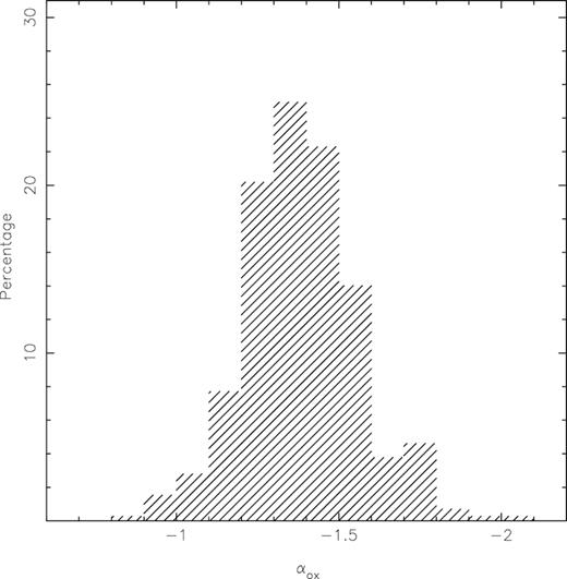
Histogram containing the distribution of the spectral index αox derived by Miller et al. (2011) for about 700 radio-intermediate and radio-loud quasars.
Regarding the metallicity, Dors et al. (2014) found that the C43 index is bivaluated, yielding one lower branch for (Z/Z⊙) ≲ 0.2 and an upper branch for |$(\mathrm{\mathit{ Z}/Z}_{\odot }) \: \gtrsim \: 0.2$|. This problem is also present in the classical Z–R23 calibration (Pagel et al. 1979) for star-forming regions and this degeneracy can be broken by using the [N ii] λ6584/[O ii] λ3727 emission-line ratio (Kewley & Ellison 2008). Due to the small number of measurements of UV emission lines in most of the AGN spectra, the degeneracy in C43 and N v/He ii calibrations can only be eliminated based on physical reasons. Studies of the NLRs of nearby Seyfert 2 AGNs (e.g. Storchi-Bergmann et al. 1998; Groves, Heckman & Kauffmann 2006; Dors et al. 2015; Castro et al. 2017; Revalski et al. 2018a,b; Thomas et al. 2018) and of objects at high redshift (e.g. Nagao et al. 2006; Dors et al. 2014; Matsuoka et al. 2009, 2018) have showed that metallicities of AGNs are generally higher than (Z/Z⊙) = 0.2. Cosmological simulations (see fig. 10 of Dors et al. 2014) and chemical evolution models (Mollá & Díaz 2008) do not predict low metallicities for the nuclear regions of galaxies (including AGNs). Besides, Matsuoka et al. (2018) derived a relation between the stellar mass of galaxies containing type-2 AGNs and their NLR metallicities, which were derived using a comparison between the observational intensities of C iv/He ii and C iii]/He ii line ratios and their photoionization model-predicted values. These authors found two metallicity values for galactic stellar masses log(M⋆/M⊙) between 11 and 11.5, and they pointed out that the lowest metallicity solution (Z/Z⊙ ≲ 0.2) is implausible since a significant decrease of metallicity with the stellar mass would be obtained. As these authors remarked, this behaviour has not been reported for any galaxy population at any redshift, and has not been reproduced by any model or cosmological simulation. Therefore, we adopted only metallicity values higher than (Z/Z⊙) = 0.2 for our AGN models, i.e. we estimated the metallicities using the upper branch of the relation of the metallicity with the C43 index and with N v/He ii emission-line ratio. Assuming a solar oxygen abundance 12 + log(O/H)⊙ = 8.69 (Alende Prieto, Lambert & Asplund 2001), we considered the following values for the metallicity in relation to the solar one (Z/Z⊙): 0.2, 0.5, 0.75, 1.0, 1.5, 2.0, and 4.0.
Regarding the nitrogen and carbon secondary nucleosynthesis elements, their abundance in relation to the oxygen abundance (or metallicity) is poorly known for AGNs. In fact, the unique quantitative nitrogen abundance estimation for AGNs is the one performed by Dors et al. (2017) for a small sample of Seyfert 2 galaxies. The predicted C43 and N v/He ii ratios are dependent on the assumed C–O and N–O relations, respectively. Hence, the derived metallicities are also dependent on the assumed relations. Thus, we performed several simulations in order to try to estimate these relations.
In Fig. 2 (left-hand panels), the diagrams N v/He ii versus C iii]/C iv (lower panel) and C43 versus C iii]/C iv (upper panel) containing the observational data listed in Table 1 and the photoionization model results (Grid-1) are shown. We can see that the predicted intensities of N v/He ii and C43 are not in agreement with the observed ones.
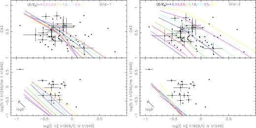
Diagrams containing observational data and photoionization model results. The points represent the observational data listed in Table 1. The curves represent the photoionization model results described in Section 2.2, where the solid lines connect models with equal metallicity (Z) as indicated. Left-hand panel: photoionization model results assuming the N–O (equation 3) and C–O (equation 4) relations proposed by Dors et al. (2017) and Dopita et al. (2006), respectively. The arrow indicates the direction in which the number of ionizing photons increases in the models. Right-hand panel: same as the left-hand panel but assuming the N–Z relation (equation 6) proposed by Hamann & Ferland (1993) and |$\rm C/H=(\mathit{ Z}/Z)_{\odot } \times (C/H)_{\odot }$|.
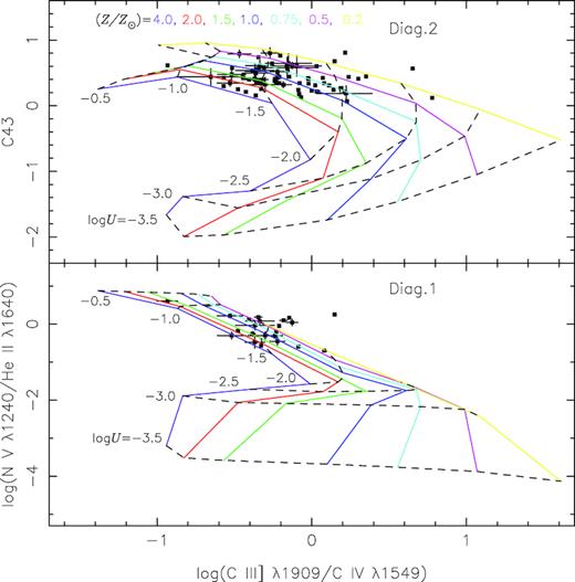
Diagrams containing observational data and the best solution for the photoionization model results, i.e. assuming in the models the relations |$\mathrm{N/H=\, 4.5} \times (\mathrm{\mathit{ Z}/Z}_{\odot })^{1.2} \times \mathrm{(N/H)}_{\odot }$| and C/H =(Z/Z⊙) × (C/H)⊙ (see Section 2.2). The points represent the observational data listed in Table 1. The curves represent the photoionization model results described in Section 2.2, where the solid lines connect models with equal metallicity (Z) and the dashed lines connect models with equal number of ionizing photons, as indicated.
In Fig. 4, top panel, we compare the logarithm of N/O abundance ratio as a function of 12 + log(O/H) (which traces the metallicity) assumed in our models (|$\mathrm{N/H=\, 4.5} \times (\mathrm{\mathit{ Z}/Z}_{\odot })^{1.2} \times \mathrm{(N/H)}_{\odot }$|) with estimations for NLRs of Seyfert 2 galaxies at z < 0.1 from Dors et al. (2017), for H ii regions calculated through the Te-method by Esteban et al. (2002, 2009, 2014), García-Rojas & Esteban (2007), López-Sánchez et al. (2007), Berg et al. (2016), and Pilyugin & Grebel (2016),1 and for the broad-line regions (BLRs) of quasars derived by Uomoto (1984) through detailed photoionization models. Since Uomoto (1984) did not derive the metallicity, i.e. only the N/C and O/C abundance ratios were estimated, his estimations are presented by a hatched area. We can see that our assumed values are in agreement with those for BLRs of quasars and they are higher than the ones for Seyfert 2 and H ii regions.
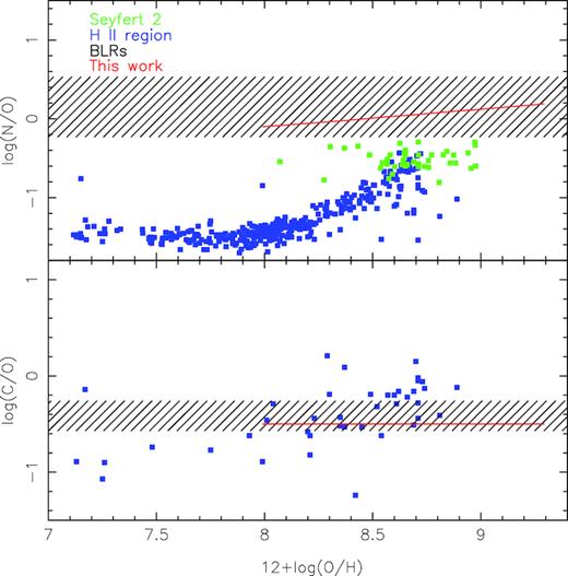
log(N/O) and log(C/O) versus 12 + log(O/H) for different kinds of objects, as indicated. The green points represent abundance ratios for NLRs of Seyfert 2 AGNs at z < 0.1 from Dors et al. (2017). The blue points represent direct estimations of abundance ratios for star-forming regions taken from Esteban et al. (2002, 2009, 2014), García-Rojas & Esteban (2007), López-Sánchez et al. (2007), Berg et al. (2016), and Pilyugin & Grebel (2016). The hatched areas represent the range of log(N/O) and log(C/O) abundance values derived for BLRs of quasars and based on detailed photoionization models by Uomoto (1984). The red lines represent the relations assumed in our models.
Also in Fig. 4, bottom panel, we compare the log(C/O) as a function of 12 + log(O/H) assumed in our models, (i.e. a fixed value |$\rm \log (C/O)=-0.50$|) with values for H ii regions and BLRs of quasars taken from the same references as in the upper panel. Unfortunately, there are no carbon abundance estimation for NLRs of Seyfert 2 galaxies in the literature. We can see that the C–O relation assumed in our models is in consonance with the ones for BLRs and H ii regions. A C/O abundance fixed to the solar value was also considered by Feltre et al. (2016), who built a wide grid of models in order to identify new line-ratio diagnostics to discriminate between gas photoionized by AGNs and by hot main-sequence stars as well as to estimate the metallicity (see also Nagao et al. 2006; Dors et al. 2014; Matsuoka et al. 2018).
As was mentioned above, we consider a fixed value for the electron density (|$N_{\rm e}=500 \rm \:cm^{3}$|). Nevertheless, the electron density varies in this kind of objects (Zhang et al. 2013; Dors et al. 2014), producing uncertainties in Z estimations based on strong emission lines. In fact, Feltre et al. (2016) showed that the location of their models in diagrams containing predicted strong optical and UV emission-line ratios varies when different Ne values are assumed. Also, Nagao et al. (2006) found that metallicities based on UV emission lines are larger when high electron density values (|${\sim } 10^{5} \: \rm cm^{-3}$|) are assumed in photoionization models instead of low electron density values (|${\lesssim } \: 10^{3} \: \rm cm^{-3}$|). In order to test the Ne influence on our Z estimations, first, we construct grids of models assuming Ne = 100, 500, and 3000 |$\rm cm^{-3}$| (the range of values found for NLRs of type-2 AGNs by Dors et al. 2014) constant along the AGN radius. The results of these grids were compared with the observational data (see Section 2.1) in two diagrams (not shown) N v/He ii and C43 versus C iii]/C iv and the interpolated Z/Z⊙ value for each object of the sample was obtained. In Fig. 5, a comparison of these metallicity estimations is shown. It can be seen that slightly higher metallicity values are derived when higher Ne values are assumed in the models. However, the discrepancies between the estimations are of the order of the uncertainties of these. Secondly, we consider models with the density ranging along the AGN radius. Revalski et al. (2018a) obtained spatially resolved optical data of the nuclear region of the Seyfert 2 galaxy Markarian 573. These authors found a density profile in the NLR of this object, with a central electron density peak of about 3000 |$\rm cm^{-3}$| and a decrease in this value following a shallow power law, i.e. Ne ∝ r−0.5, r being the distance to the AGN centre. We built photoionization models assuming this radial density profile (not shown) and the intensities of UV emission-lines predicted by these are about the same ones of models with Ne constant along r. Therefore, electron density variations have an almost negligible influence in the considered line ratios for our estimations.
![Comparison between metallicity (Z/Z⊙) estimations for the sample of objects (see Section 2.1) obtained from the diagrams (not shown) N v/He ii versus C iii]/C iv (left-hand panel) and C43 versus C iii]/C iv (right-hand panel) considering grid of models assuming electron density Ne = 100, 500, and 3000 $\rm cm^{-3}$, as indicated in the axis labels.](https://oup.silverchair-cdn.com/oup/backfile/Content_public/Journal/mnras/486/4/10.1093_mnras_stz1242/1/m_stz1242fig5.jpeg?Expires=1750244122&Signature=ZmiGtt6eO3P4rxc9-UPTd6I8zXUD0WzMjHnVp9oRSuxf0GDI-FT~WRJXdPOqpd6r1eZlkLrqzIyTyjcbHzLD8HKtECNaRhW748QujNgECLFhxB6eyu2Bx9MIB7amOHxxBaRUycBwpCVRrDVkpunDf0S~bpPjoZuVzSm7PUPweEXljyb3Zu~83XyNWYjLqxpGvhdIcuNvfE66rxThNKJgcvKnVnPJHV2eiWzNVwibTH8N~qtHE8IxFO9d4a2lxo0iwLrdLYPkKcZO8qABj9t7ym19D~7Gb4L~yTy~c~6gkatNEReatBGCQXaxqFckO53bVfTqF7IG6y9hz0LMTOQ-Hw__&Key-Pair-Id=APKAIE5G5CRDK6RD3PGA)
Comparison between metallicity (Z/Z⊙) estimations for the sample of objects (see Section 2.1) obtained from the diagrams (not shown) N v/He ii versus C iii]/C iv (left-hand panel) and C43 versus C iii]/C iv (right-hand panel) considering grid of models assuming electron density Ne = 100, 500, and 3000 |$\rm cm^{-3}$|, as indicated in the axis labels.
Finally, we also explore the dependence of the spectral index αox on our metallicity estimations. To do this, we built grids of photoionization models assuming three different index values: αox = −2.0, −1.4, and −0.8. This is the range of αox values found by the observational study carried out by Miller et al. (2011) and represented in Fig. 1. The SED with αox = −2.0 represents an ionizing source with a very soft spectrum, yielding models with very low ionization degree and, hence, with emission-line ratios largely discrepant from those of the observational sample. It must be noted that very few (|${\lesssim } 1{{\ \rm per\ cent}}$|) objects studied by Miller et al. (2011) have αox near to −2.0. The results of these grids were compared with the observational data in two diagrams (not shown) N v/He ii and C43 versus C iii]/C iv and the interpolated Z/Z⊙ values were estimated for each object. In Fig. 6, a comparison of these metallicity estimations is shown. It can be seen that when αox = −0.8 is considered higher (|${\sim } 90{{\ \rm per\ cent}}$|) metallicity values are obtained in comparison with those estimated by models with αox = −1.4. However, as can be seen in Fig. 1, very hard SEDs (αox < −1.0) are derived only for few (|${\sim } 2{{\ \rm per\ cent}}$|) objects and most part of AGNs presents αox around −1.4. Therefore, we conclude that our metallicity estimations based on the models with αox = −1.4 (see Fig. 3) seem to relate to the real metallicity of the observed regions.
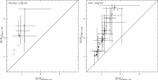
Same as Fig. 5 but for grids of models assuming αox equal to −1.4 and −0.8.
Thomas et al. (2018) presented a Bayesian code that implements a general method of comparing observed emission-line fluxes to photoionization model grids representing AGNs (see also Blanc et al. 2015) and taking into account a large range of nebular parameters (e.g. gas pressure, depletions on to dust grains) and SEDs of the ionizing source. Basically, this method determines the probability of that a set of model parameter values is representative of a set of observational data of a given object. Applying this method, Thomas, Kewley & Dopita (2019) found a correlation between the mass of the host galaxy and the metallicity of the AGN (see also Matsuoka et al. 2018) for a sample from the SDSS (York et al. 2000). Thomas et al. (2019) pointed out that their sophisticated analysis produces almost an identical mass–metallicity relation to the one derived from the Z–N2O2 calibration obtained by Castro et al. (2017) and based on similar photoionization models (and methodology) applied in the present work (see also Mignoli et al. 2019). Therefore, metallicity estimations based on simplified photoionization models seem to be reliable.
3 RESULTS
The diagrams in Fig. 3, N v/He ii versus C iii]/C iv (Diag. 1, lower panel) and C43 versus C iii]/C iv (Diag. 2, upper panel) were used to calculate the logarithm of the number of ionizing photons [|$\log (Q(\rm H)$|] and the metallicity (Z/Z⊙) for each object in our sample applying a linear interpolation between the models. These results are listed in Table 1. The interpolated parameters together with the observational line ratios for each object were used to obtain semi-empirical calibrations.
![Upper panel: bi-dimensional calibrations between the metallicity (Z/Z⊙), log(N v λ1240/He ii λ1640) and log(C iii] λ1909/C iv λ1549) line ratios. The points represent metallicity estimations for objects listed in Table 1 and obtained using the lower panel of Fig. 3 as described in Section 3. The colour coding indicates values of the logarithm of the ionization parameter (log U) estimated for each object. The surface represents the best fit to the points and its expression is given in equation (7). Lower panel: calibration between the metallicity (Z/Z⊙), C43 = log[(C iv λ1549 + C iii] λ1909)/He ii λ1640], and log(C iii] λ1909/C iv λ1549) line ratios using metallicities estimations obtained using the upper panel of Fig. 3 as described in Section 3. The surface represents the best fit to the points and its expression is given in equation (8).](https://oup.silverchair-cdn.com/oup/backfile/Content_public/Journal/mnras/486/4/10.1093_mnras_stz1242/1/m_stz1242fig7.jpeg?Expires=1750244122&Signature=nljNpK7isUm8Iu-Zwpn~hZeAFNZB0ieojPz9xXUEp241AvlJDLYU1fSflqqeC2TkLtOKgYC9NY4~x7roujJY~V4Y7BNYUKq5wrMgYnj84vJ9P00V8VWOYAQ5DTSEkSbWzcQVnBubc2VkvEhYAhriITKqpbZNiwOfyZV4zhAZF9EXAZrd9W2JxzKaYFqnT5I7gDZ0Nvba5mMZyhu7AWDlpavMkHgBLq9yLcy1Mo3l2i2jZf9oZPe0xo5RRUp40qoAxiJShN1rH66GNqdJvYrt3MJi3y2H1HTyoKqpx2RP2sjdQrQM-GlJZ3Ug1GvNVmO7qTBSaLCzKTzaYqMQTn-WwA__&Key-Pair-Id=APKAIE5G5CRDK6RD3PGA)
Upper panel: bi-dimensional calibrations between the metallicity (Z/Z⊙), log(N v λ1240/He ii λ1640) and log(C iii] λ1909/C iv λ1549) line ratios. The points represent metallicity estimations for objects listed in Table 1 and obtained using the lower panel of Fig. 3 as described in Section 3. The colour coding indicates values of the logarithm of the ionization parameter (log U) estimated for each object. The surface represents the best fit to the points and its expression is given in equation (7). Lower panel: calibration between the metallicity (Z/Z⊙), C43 = log[(C iv λ1549 + C iii] λ1909)/He ii λ1640], and log(C iii] λ1909/C iv λ1549) line ratios using metallicities estimations obtained using the upper panel of Fig. 3 as described in Section 3. The surface represents the best fit to the points and its expression is given in equation (8).
![As in Fig. 7 but for log U as a function of the logarithm of C iii] λ1909/C iv λ1549 emission-line ratio. The line represents the best fit.](https://oup.silverchair-cdn.com/oup/backfile/Content_public/Journal/mnras/486/4/10.1093_mnras_stz1242/1/m_stz1242fig8.jpeg?Expires=1750244122&Signature=kTCWcmY0LAtsWt7kOgHkRjYrfsxsXantC4y2VU6-mbqs0LFhtNR7tZujRqYARhVvpAAQPBy08WaeGDtzHfm8IpvcrpEW2uVidav6lc35AANEO7InDj92I70nRBqcr5KYUdQ0-lMKLrZP~BYmuxHvcttGIbGi~nKu-F3P5MJqm7qknwu8lo6OlpqVMiUWOiPYsbXzk8xA1ZhrJKCs0uxIusykOSF22HUhycUb64Ln4e4JkQtrJPce1QJ6uCx1TS2gijttsqfJEKnYDQPgkOcE7rHiKqjqap9elBk2U52vBBceDvypf2oG2NsqhVCUsUEbSAXrykrR5QbBITBJoMIGBg__&Key-Pair-Id=APKAIE5G5CRDK6RD3PGA)
As in Fig. 7 but for log U as a function of the logarithm of C iii] λ1909/C iv λ1549 emission-line ratio. The line represents the best fit.
In Fig. 9, the logarithms of the ionization parameter obtained with the diagnostic diagrams presented in Fig. 3 (Diag. 1 and Diag. 2) and listed in Table 1 are compared. This figure shows a very good agreement between both estimations.

4 DISCUSSION
4.1 Metallicity in narrow- and broad-line regions
The first metallicity estimations in BLRs of AGNs based on UV emission lines were obtained by Shields (1976) and Davidson (1977), who used the initial photoionization models (see Davidson 1972; Shields 1974; Baldwin & Netzer 1978) to investigate which combinations of line ratios are the most appropriate to estimate abundance ratios (e.g. N/C and O/C). Later, Uomoto (1984) obtained UV spectra of a sample of six quasars (|$1.6 \: \lt \, z \: \lt 2.1$|) and, fitting photoionization models to the observational line measurements, Uomoto found about solar oxygen abundances and a slight enhancement of nitrogen abundances for two of these quasars. Other studies, as for example Hamann et al. (1997), concluded that BLRs, in fact, present supersolar abundances (Z > 5 Z⊙) and an enhancement of N abundances (see also Peimbert 1968; Alloin 1973; Storchi-Bergmann & Pastoriza 1990; Storchi-Bergmann 1991; Dietrich et al. 2003; Bradley, Kaiser & Baan 2004). More recently, Sameshima, Yoshii & Kawara (2017) derived the metallicity, traced by the Fe/H and Mg/Fe abundance ratios, in the BLRs of a sample of about 17 500 quasars (0.7 ≲ z ≲ 1.7), whose observational data were taken from the SDSS (York et al. 2000). To obtain the metallicity, these authors compared observational fluxes and equivalent widths of Fe ii (calculated by integrating the fitted Fe ii template in the |$\rm 2200\!-\!3090\, \mathring{\rm A}$| wavelength range) and Mg ii λ2798 lines with photoionization model results. They found that the majority of the objects have oversolar metallicities with a median value of Z ≈ 3 Z⊙, reaching up to (Z/Z⊙) ∼ 100 (see also Dietrich & Wilhelm-Erkens 2000; Hamann et al. 2002; Batra & Baldwin 2014).
In order to compare our NLRs Z estimations with those for BLRs, a histogram containing the metallicity distribution for our sample, derived using equation (8), and the results of Sameshima et al. (2017) is presented in Fig. 10. We limited their estimations to |$(\mathrm{\mathit{ Z}/Z}_{\odot }) \:\leqq \: 10$| since few objects present higher metallicities. In Fig. 10, the NLR metallicity results derived by Castro et al. (2017), from a semi-empirical calibration between Z and the optical ratio N2O2 = log([N ii] λ6584/[O ii] λ3727), are also shown. We found that the majority (|${\sim } 60 {{\ \rm per\ cent}}$|) of the NLRs metallicity estimations based on the C43 are in the 0.5 ≲ (Z/Z⊙) ≲ 1.5 range, with a median value of <Z/Z⊙ > ∼1.1. Very different metallicity distributions are found for NLRs and BLRs, the latter being more extended and with a median value higher, by a factor of 2–3, than the former. This difference could be probably due to the fact that broad lines originate in a small region with a radius lower than 1 pc (Kaspi et al. 2000; Suganuma et al. 2006), which may evolve more rapidly than the NLRs (Matsuoka et al. 2018). As can be seen in Fig. 10, our metallicity estimations follow the same distribution than those derived by Castro et al. (2017) for the NLRs of Seyfert 2 AGNs, who found metallicities in the 0.7 ≲ (Z/Z⊙) ≲ 1.2 range for most of their objects.

Histograms containing NLRs and BLRs metallicity distributions. The red (empty-filled) histogram represents NLRs metallicity distribution for our sample (0.04 < z < 4.0) and using the equation (8). The black histogram (with slant-filled pattern) represents NLRs metallicity distribution for a sample of Seyfert 2 AGNs (z < 0.1) derived using a semi-empirical calibration proposed by Castro et al. (2017). The Cyan histogram (with x-filled pattern) represents BLRs metallicity distribution for a sample of quasars (|$1.6 \: \lt \, z \: \lt 2.1$|) derived by Sameshima et al. (2017).
4.2 Metallicity estimations from distinct calibrations
Previous studies of metallicities in AGNs (e.g. Shemmer & Netzer 2002; Dietrich et al. 2003; Dhanda et al. 2007) and in star-forming regions (e.g. Kewley & Ellison 2008; López-Sánchez & Esteban 2009; Dors et al. 2011) have shown that different methods or different calibrations of the same index provide different metallicity values, with discrepancies of up to 1.0 dex.
In order to compare the estimations from our two calibrations, in the bottom panel of Fig. 11, Z estimations for the objects in our sample obtained from the bi-parametric calibration |$(\mathrm{\mathit{ Z}/Z}_{\odot })=f({\rm{N}}\,{\rm{\small V}}/{\rm{He}}{ \,\rm{\small II}},{\rm{C}}{\rm\,{\small III}}]/ {\rm{C}}{\rm\,{\small IV}})$| (equation 7) are plotted against the estimations via |$(\mathrm{\mathit{ Z}/Z}_{\odot })=f(\rm C43,{\rm{C}}{\rm\,{\small III}}]/ {\rm{C}}{\rm\,{\small IV}})$| (equation 8). It can be seen that, despite the large scattering and the few number of points, the estimations are in consonance with each other.
![Comparison between NLRs metallicity estimations for the objects in our sample obtained through distinct calibrations. The solid lines represent the one-to-one relation between the estimations. Bottom panel: estimations via $\mathrm{\mathit{ Z}/Z}_{\odot }=f({\rm{N}}\,{\rm{\small V}}/{\rm{He}}{ \,\rm{\small II}},{\rm{C}}{\rm\,{\small III}}]/ {\rm{C}}{\rm\,{\small IV}})$ (equation 7) versus those via $\mathrm{\mathit{ Z}/Z}_{\odot }=f({\rm C43},{\rm{C}}{\rm\,{\small III}}]/ {\rm{C}}{\rm\,{\small IV}})$ (equation 8). Upper panel: estimations via the theoretical calibration $(\mathrm{\mathit{ Z}/Z}_{\odot })=f({\rm C43},{\rm{C}}{\rm\,{\small III}}]/ {\rm{C}}{\rm\,{\small IV}})$ proposed by Dors et al. (2014) versus those via $\mathrm{\mathit{ Z}/Z}_{\odot }=f({\rm C43},{\rm{C}}{\rm\,{\small III}}]/ {\rm{C}}{\rm\,{\small IV}})$ (equation 8).](https://oup.silverchair-cdn.com/oup/backfile/Content_public/Journal/mnras/486/4/10.1093_mnras_stz1242/1/m_stz1242fig11.jpeg?Expires=1750244122&Signature=sujDRrEUqOWR6ghX5lLVJ79mbL3xevXWwp4Igt9E560dbypwgxkwSzjSr95rA-slcncn-3jA-hTFVSMLrcKWMo~TN48eqDz~bF5~C92MRtGEKItyEWKEy24Vm~V6m8i1M77SkBOEtoSbQGcINhYuAijn4DNW3LIU5~CwdaVxnI4O1DWLssu4DNyl-qIIUQsrrnMNlsVJ23HlIQFnDx0px10GTxdcI6XV5wj2gOSSSeT2t3KUg3T3X2Gs-pUPjKaGX-YQYnKpfBvNQUdbO0d2wj~HK5EqOWSYnZPGqjogB6hhkWGEmrP4eI7aW~QXths8KcXiXqXWAkoajARW5S1bgg__&Key-Pair-Id=APKAIE5G5CRDK6RD3PGA)
Comparison between NLRs metallicity estimations for the objects in our sample obtained through distinct calibrations. The solid lines represent the one-to-one relation between the estimations. Bottom panel: estimations via |$\mathrm{\mathit{ Z}/Z}_{\odot }=f({\rm{N}}\,{\rm{\small V}}/{\rm{He}}{ \,\rm{\small II}},{\rm{C}}{\rm\,{\small III}}]/ {\rm{C}}{\rm\,{\small IV}})$| (equation 7) versus those via |$\mathrm{\mathit{ Z}/Z}_{\odot }=f({\rm C43},{\rm{C}}{\rm\,{\small III}}]/ {\rm{C}}{\rm\,{\small IV}})$| (equation 8). Upper panel: estimations via the theoretical calibration |$(\mathrm{\mathit{ Z}/Z}_{\odot })=f({\rm C43},{\rm{C}}{\rm\,{\small III}}]/ {\rm{C}}{\rm\,{\small IV}})$| proposed by Dors et al. (2014) versus those via |$\mathrm{\mathit{ Z}/Z}_{\odot }=f({\rm C43},{\rm{C}}{\rm\,{\small III}}]/ {\rm{C}}{\rm\,{\small IV}})$| (equation 8).
In the top panel of Fig. 11, the estimations from the semi-empirical calibration |$(\mathrm{\mathit{ Z}/Z}_{\odot })=f({\rm C43},{\rm{C}}{\rm\,{\small III}}]/ {\rm{C}}{\rm\,{\small IV}})$| (equation 8) are compared to those derived via the theoretical relation by Dors et al. (2014), where it can be seen that the later one produces Z values higher than the former, mainly for the high-metallicity regime. This difference is probably due to Dors et al. (2014) did not deeply explore the dependence between the metallicity and the U–C iii/C iv relation. Since the semi-empirical and bi-parametric calibrations (equations 7 and 8) are derived taken into account observational data, they are, in principle, more robust and confident than the purely theoretical calibration derived by Dors et al. (2014).
The estimations using these optical calibrations are compared with the ones via equations (7) and (8) in Table 2. We can see that the f(C43,C iii]/C iv) relation (equation 8) produces the closest values to the ones from the optical calibrations (equations 10 and 11). Nevertheless, it must be noted that only three objects do not constitute a statistically significant comparison sample.
4.3 Mass–Metallicity relation

M–Z relation for type-2 AGNs. Metallicity values were calculated via equation (7) (bottom panel) and equation (8) (upper panel). The solid lines represent the linear regressions (equations 13 and 14). In the upper panel, the dashed line represents the linear regression without taking into account the more massive object (equation 15). The arrows indicate that only the upper limit of the stellar mass was quoted in the literature (see Table 1).
Unfortunately, as can be seen in the lower panel of the Fig. 12, we have a small number of objects with metallicities derived from equation (7) and with estimations of their stellar masses. Hence, we consider that the M–Z relation given by equation (13) is not statistically significant; hereafter, we will only discuss the M–Z relation given by equation (15).
In Fig. 13, the M–Z relation given by equation (15) is compared with the relation obtained by Thomas et al. (2019) for local (z < 0.2) Seyfert 2 AGNs (in the mass interval 10.1 < [log (M∗/M⊙)] < 11.3), and with M–Z relations for star-forming galaxies at different redshift ranges derived by Maiolino et al. (2008). We can see a difference between our M–Z relation and the one derived by Thomas et al. (2019). Taking into account the very different redshift ranges between the Thomas and collaborators and our samples, this difference in the M–Z relation could be explained by the evolution of this relation with the redshift. This interpretation is based on the observed gradual declination of the metallicity with the redshift for a given mass in SF galaxies from the Maiolino and collaborators work as can be seen in Fig. 13 (see also Savaglio et al. 2005; Erb et al. 2006; Yabe et al. 2014; Ly et al. 2016). It is noticeable that our relation (equation 15) seems to complement the one derived by Maiolino et al. (2008) for z ∼ 3.5 towards higher masses. It is worth emphasizing that a larger sample of AGNs with metallicity estimations and with estimations of the stellar mass of the host galaxies, mainly covering a wider range in masses, is needed to improve the M–Z relation.

5 CONCLUSION
We compared the observational intensities of UV emission lines with results of photoionization models in order to obtain two semi-empirical calibrations between the metallicity of the NLR of type-2 active galactic nuclei and the N v λ1240/He ii λ1640, C43 = log[(C iv λ1549 + C iii] λ1909)/He ii λ1640], and C iii] λ1909/C iv λ1549 emission-line ratios. We also derived a metallicity-free calibration between the ionization parameter and the C iii] λ1909/C iv λ1549 emission-line ratio. We showed that the metallicity in NLRs of AGNs is lower by a factor of 2–3 than the metallicity in BLRs. Using the derived calibrations, we confirmed the recent result of the existence of a relation between the stellar mass of the host galaxy and its NLR metallicity. We were able to derive two M–Z relations even though we consider that one of them is not statistically significant due to the small number of objects available to derive it. The adopted M–Z relation was obtained using type-2 AGNs at z between 1.6 and 3.8. Comparing our relation with the ones derived by Maiolino et al. (2008) for star-forming galaxies at high redshifts, we found that the M–Z relation of type-2 AGNs seems to complement the sequences towards higher masses following the same trend.
ACKNOWLEDGEMENTS
We are grateful to the anonymous referee for her/his very useful comments and suggestions that helped us to clarify and improve this work. OLD and ACK are grateful to FAPESP and CNPq. AFM is grateful to CAPES. MVC and GFH are grateful to CONICET. OLD is grateful to Dr. Sameshima and Dr. Miller for making their BLR metallicity estimations and αox values available, respectively.
