


Abstract
The extreme infrared (IR) luminosity of local luminous and ultraluminous IR galaxies (U/LIRGs; |$11 \lt \log L_{\rm IR}\,/\, L_\odot \lt 12$| and |$\log L_{\rm IR}\,/\, L_\odot\,\, \gt\,\, 12$|, respectively) is mainly powered by star formation processes triggered by mergers or interactions. While U/LIRGs are rare locally, at z > 1, they become more common, dominate the star formation rate (SFR) density, and a fraction of them are found to be normal disc galaxies. Therefore, there must be an evolution of the mechanism triggering these intense starbursts with redshift. To investigate this evolution, we present new optical SWIFT integral field spectroscopic H α + [N ii] observations of a sample of nine intermediate-z (0.2 < z < 0.4) U/LIRG systems selected from Herschel 250 |$\mu$|m observations. The main results are the following: (a) the ratios between the velocity dispersion and the rotation curve amplitude indicate that 10–25 per cent (1–2 of 8) might be compatible with being isolated discs, while the remaining objects are interacting/merging systems; (b) the ratio between un-obscured and obscured SFR traced by H α and LIR, respectively, is similar in both local and these intermediate-z U/LIRGs; and (c) the ratio between 250 |$\mu$|m and the total IR luminosities of these intermediate-z U/LIRGs is higher than that of local U/LIRGs with the same LIR. This indicates a reduced dust temperature in these intermediate-z U/LIRGs. This, together with their already measured enhanced molecular gas content, suggests that the interstellar medium conditions are different in our sample of intermediate-z galaxies when compared to local U/LIRGs.
1 INTRODUCTION
Discovered in large numbers by the Infrared (IR) Astronomical Satellite (IRAS), luminous (|$11\,\,\lt\,\, \log L_{\rm IR(8-1000\mu m)}\,/\, L_{\odot }\,\, \lt\,\, 12$|; LIRGs) and ultraluminous IR galaxies (|$\log L_{\rm IR(8-1000\mu m)}\,/\, L_\odot \,\,\gt\,\, 12$|; ULIRGs) are amongst the most intensely star-forming galaxies in the Universe. While scarce locally, they are far more numerous at high redshifts and are responsible for about 50 per cent of the total star formation rate (SFR) density at z > 1 (e.g. Le Floc’h et al. 2005; Pérez-González et al. 2005; Caputi et al. 2007; Magnelli et al. 2011). As such, U/LIRGs represent an important population for understanding galaxy evolution.
In the local Universe, U/LIRGs are primarily found in interacting and/or merging systems. They exhibit a wide range of morphologies suggesting different dynamical phases ranging from isolated discs in low-luminosity LIRGs to strongly interacting galaxies and fully merged systems (Kim, Veilleux & Sanders 1998; Farrah et al. 2001, 2003, 2013; Veilleux, Kim & Sanders 2002; Arribas et al. 2008; Bellocchi et al. 2013; Kim et al. 2013). It is now well established that interactions and mergers are responsible for their intense star-forming activity specially at the higher end of the luminosity range (Melnick & Mirabel 1990; Clements et al. 1996; Bushouse et al. 2002). The spectral energy distributions (SEDs) of U/LIRGs are dominated by dust thermal emission arising from reprocessing of ultraviolet radiation produced either by young massive stars or an active galactic nucleus (AGN) with dust temperatures in the range of 40–60 K (Symeonidis et al. 2010; Clements et al. 2018). Local U/LIRGs have high star formation efficiencies (SFEs; defined as the ratio of the total IR luminosity over the molecular gas mass) of the order of >100 |$L_{\odot }\,/\, M_{\odot }$| (Gao & Solomon 2004) and are characterized by compact star-forming regions, confined within the central kiloparsec of the merging systems (Iono et al. 2009; Elbaz et al. 2011; Rujopakarn et al. 2011). However, the star-forming regions are more spatially extended in isolated LIRGs and LIRGs in weakly interacting galaxy groups (see Alonso-Herrero et al. 2006; Pereira-Santaella et al. 2015).
At higher redshifts, however, the properties of U/LIRGs appear to diverge from those of their local counterparts. Recent morphological studies have found that high-z ULIRGs appear to be a mixture of merging/interacting systems and disc galaxies (e.g. Kartaltepe et al. 2012; Kaviraj et al. 2013; Alcorn et al. 2018; Wisnioski et al. 2018). Continuous gas accretion via cold gas flows and minor mergers have been proposed as mechanisms to supply gas directly to the centre of galaxies to maintain the high levels of star formation (SF) observed in these high-z disc galaxies (Ocvirk, Pichon & Teyssier 2008; Dekel, Sari & Ceverino 2009). In addition, studies based on Spitzer and Herschel measurements have shown that the IR SEDs of high-z U/LIRGs are more similar to those of local galaxies of lower luminosity, exhibiting stronger polycyclic aromatic hydrocarbon features (Pope et al. 2006; Farrah et al. 2008) and colder dust temperatures (e.g. Muzzin et al. 2010; Magdis et al. 2012; Symeonidis et al. 2013) than local U/LIRGs. Engelbracht et al. (2008) suggested that such differences in the SEDs of local and high-z U/LIRGs are qualitatively consistent with decreased metallicities by a factor of 1.5–2, while differences in the physical size of the star-forming regions have also been implicated.
To fully understand the evolution of the ULIRG phenomenon, studies of the properties of U/LIRGs in the 0.2 < z < 1 redshift range are necessary. Incidentally, this is the era when the Universe experienced a strong decrease in its SFR density (Magnelli et al. 2011). For this purpose, we have defined a sample of intermediate-z U/LIRGs originally drawn from Herschel observations of well-studied fields in the sky, including Bootes, Extended Groth Strip, the Cosmic Evolution Survey, and the Hubble Deep Field North. A detailed study of the SEDs, the properties of their interstellar medium (ISM), and their molecular gas content have already been presented in Rigopoulou et al. (2014) and Magdis et al. (2014). Spatially resolved kinematic studies of intermediate-z U/LIRGs are a powerful diagnostic of the main source of dynamical support as they allow us to distinguish between relaxed virialized systems and merger events. The morphology of lower luminosity star-forming galaxies at intermediate redshifts shows that only a few per cent show signs of interaction (e.g. Lee et al. 2017). Similarly, the distance to the main sequence seems to be enhanced by galaxy interactions. However, the SFE seems to be independent of the interaction stage (e.g. Bauermeister et al. 2013; Lee et al. 2017).
In this paper, we present optical (H α +[N ii] plus adjacent continuum) integral field spectroscopy (IFS) measurements of nine systems observed with the SWIFT spectrograph (Thatte et al. 2006). We focus on the study of the optical emission line spectra and kinematics probing the prevalence of AGN amongst the sample as well as the mechanism (e.g. merger versus secular evolution) that drives SF activity in U/LIRGs between the present day and z ∼ 1.
This paper is organized as follows: The SWIFT sample and observations are described in Section 2. The analysis of the H α and [N ii] emission and the kinematic models is presented in Section 3. In Section 4, we compare the properties of our sample of intermediate-z U/LIRGs and local U/LIRGs. In Section 5, we summarize the main results of this work. Throughout this paper, we assume the following cosmology: H0 = 70 km s−1 Mpc−1, Ωm = 0.3, and ΩΛ = 0.7.
2 OBSERVATIONS AND DATA REDUCTION
2.1 The sample
We selected the targets from the sample of intermediate-z U/LIRGs presented in Rigopoulou et al. (2014) and Magdis et al. (2014). In brief, this sample of intermediate-z U/LIRGs was originally selected from the photometric catalogues from the Herschel Multitiered Extragalactic Survey (Oliver et al. 2012) by applying the following two criteria: first, the sources had to have S250 >150 mJy and secondly, their redshift (photometric or spectroscopic) had to be 0.2 < z < 0.8. The flux cut was imposed so that the sources would be IR luminous (LIR > 1011.5 L⊙), while the redshift cut ensured that the far-IR line [C ii] 158 |$\mu$|m line would shift in the wavelength range covered by the Spectral and Photometric Imaging REceiver-Fourier Transform Spectrometer (SPIRE-FTS; Griffin et al. 2010) on board Herschel. No other criteria such as optical colours, morphologies, stellar mass, or presence of an AGN were taken into consideration. This is particularly important, as one of the goals of the current investigation is to establish whether intermediate-z U/LIRGs are major mergers/interacting systems as is the case for most of their local counterparts. This initial selection resulted in a sample of 21 sources in the redshift range 0.219 < z < 0.887. Amongst the targets, there were two lensed sources XMM1 (zspec = 2.308) and SWIRE6 (zspec = 2.957), which were initially selected as the zspec = 0.502 and zspec = 0.584 foreground galaxies of the lensed SMGs HXMM01 (Fu et al. 2013) and HLSW-01 (Rigopoulou et al. 2018). All intermediate-z U/LIRGs were subsequently targeted with the SPIRE-FTS. Of those, [C ii] emission was detected in 17 of them. Details of the spectroscopic CO follow-up and SED modelling of this sample can be found in Magdis et al. (2014).
Most of the objects in the parent sample of intermediate-z U/LIRGs are star-forming main-sequence galaxies (see Fig. 1 and Magdis et al. 2014). This figure shows that our sample has SFEs (i.e. LIR /|$L^{\prime }_{\rm CO}$| ratio) similar to those of disc galaxies (the black circles), and lie close to the relation observed in main-sequence galaxies (the black solid line). For comparison, local U/LIRGs (the orange circles) and intermediate-z ULIRGs selected with IRAS (the green squares), which are starburst objects, have higher SFEs than most of the objects in our sample.
![Infrared luminosity versus CO (1–0) luminosity for the galaxies in the parent sample of intermediate-z U/LIRGs with CO and [C ii] observations (the red circles; Magdis et al. 2014; Rigopoulou et al. 2014). The black circles are disc galaxies with 0.3 < z < 2.5 (Daddi et al. 2010; Genzel et al. 2010; Geach et al. 2011), the orange circles are local U/LIRGs (Solomon et al. 1997), and the green squares are warm z ∼ 0.3 U/LIRGs selected with IRAS (Combes et al. 2011). The solid and dashed black lines represent the relation observed for main-sequence and starburst galaxies, respectively (Sargent et al. 2014).](https://oup.silverchair-cdn.com/oup/backfile/Content_public/Journal/mnras/486/4/10.1093_mnras_stz1218/1/m_stz1218fig1.jpeg?Expires=1750306014&Signature=W3ILMgq9DzVz9jV8OKJ9U1k24NkW87eOLxPnXInJ5figzxxbw3t5J3VIAjOp5YHoefNG74-xIOan6eRJJTVQtRlgKK2MzO05M7iAryC~Rl7iXRfXsWOyqG840c2R8lSsqOZc2-pzXU2j0c1EKMRjhtuUhyXtsZbXX1eYv1k7gelVAbMZv-nUBzcMwWe5EKAKCJVF4AAG~1P1Z1VaHs1MMOMCJ9l7mGKWwLory3pXTA1QN0FfCtmqWvGf6i0k5yjvOW53eBkFl5J3yLECJmO0~12gwuqQxoQ8cphPIFNNgzktMWpgarAl2EAuB2g0mhE~qQ8-TZfxBz0I4xbCt~AVUA__&Key-Pair-Id=APKAIE5G5CRDK6RD3PGA)
Infrared luminosity versus CO (1–0) luminosity for the galaxies in the parent sample of intermediate-z U/LIRGs with CO and [C ii] observations (the red circles; Magdis et al. 2014; Rigopoulou et al. 2014). The black circles are disc galaxies with 0.3 < z < 2.5 (Daddi et al. 2010; Genzel et al. 2010; Geach et al. 2011), the orange circles are local U/LIRGs (Solomon et al. 1997), and the green squares are warm z ∼ 0.3 U/LIRGs selected with IRAS (Combes et al. 2011). The solid and dashed black lines represent the relation observed for main-sequence and starburst galaxies, respectively (Sargent et al. 2014).
For this paper, we selected the nine northern intermediate-z U/LIRGs for follow-up with the SWIFT integral field spectrograph. The SWIFT sample is presented in Table 1 with the naming convention as in Magdis et al. (2014).
Sample of intermediate-z U/LIRGs.
| Name | RA a | Dec. a | z b | |${\log L_{\rm IR}\,/\, L_\odot }$| c | Separation d | Obs. date | Seeing FWHM e | SFRIR f |
|---|---|---|---|---|---|---|---|---|
| (J2000.0) | (J2000.0) | (arcsec kpc−1) | (arcsec kpc−1) | (M⊙ yr−1) | ||||
| XMM2 W | 2:19:57.30 | −5:23:48.8 | 0.199 | 11.87 | 6.9/23 | 2013-10-23 | 1.2/3.9 | 110 |
| XMM2 E | 2:19:57.72 | −5:23:51.8 | 0.200 | – | – | – | – | – |
| CDFS2 N | 3:28:18.02 | −27:43:07.5 | 0.248 | 11.83 | 6.8/27 | 2013-10-24 | 1.5/5.8 | 98 |
| CDFS2 S | 3:28:18.26 | −27:43:13.5 | 0.248 | – | – | – | – | – |
| CDFS1 W | 3:29:04.39 | −28:47:53.0 | 0.289 | 11.80 | 7.0/31 | 2013-10-25 | 1.4/6.0 | 91 |
| CDFS1 E | 3:29:04.89 | −28:47:55.5 | 0.291 | – | – | – | – | – |
| SWIRE5 Wg | 10:35:57.80 | + 58:58:46.5 | 0.195 | ⋅⋅⋅ | ⋅⋅⋅ | 2013-01-16 | 2.7/8.7 | ⋅⋅⋅ |
| SWIRE5 E | 10:35:57.99 | + 58:58:46.0 | 0.366 | 12.07 | – | – | 2.7/13.7 | 170 |
| SWIRE3 | 10:40:43.63 | + 59:34:09.2 | 0.147 | 11.61 | ⋅⋅⋅ | 2013-01-17 | 3.0/7.7 | ⋅⋅⋅ |
| SWIRE7 | 11:02:05.68 | + 57:57:40.4 | 0.414 | 12.10 | ⋅⋅⋅ | 2013-01-17 | 2.1/11 | 190 |
| BOOTES1 | 14:36:31.95 | + 34:38:29.2 | 0.351 | 12.69 | ⋅⋅⋅ | 2012-05-12 | 1.5/7.4 | ⋅⋅⋅ |
| BOOTES2 | 14:32:34.90 | + 33:28:32.2 | 0.249 | 11.90 | ⋅⋅⋅ | 2012-05-14 | 1.4/5.5 | 93 |
| FLS02 N | 17:13:31.49 | + 58:58:04.4 | 0.436 | 12.42 | 3.6/21 | 2012-05-09 | 1.6/9.0 | 380 |
| FLS02 S | 17:13:31.64 | + 58:58:01.0 | 0.437 | – | – | – | – | – |
aCoordinates from the i-band SDSS images except for the CDFS1 and CDFS2 systems for which we used the ALMA CO (3–2) emission (Rigopoulou et al., in preparation) and the R DSS image, respectively.
cTotal 8–1000 |$\mu$|m IR luminosity derived from the IR spectral energy distribution fitting (Magdis et al. 2014).
dProjected separation between the two nuclei of the system.
eSeeing FHWM measured from the telluric star observation and its equivalent linear size at distance of the observed system.
fSFR derived from the total IR luminosity using the Murphy et al. (2011) calibration (see Section 4.2). We do not compute SFRIR for SWIRE3 and BOOTES1 because they may host a bright AGN based on the broad H α emission line profile (Section 3.2) and this AGN might contribute to the observed IR luminosity.
gThis is a foreground galaxy at z = 0.195 unrelated to the ULIRG, SWIRE5 E, discussed in this paper. Note that the redshift of SWIRE5 W is coincident with the spectroscopic redshift given by Rowan-Robinson et al. (2010) for SWIRE5.
2.2 Optical integral field spectroscopy
We obtained optical I- and z-band optical IFS of the U/LIRGs in our sample using the SWIFT instrument mounted on the 5.1 m Hale Telescope at the Palomar Observatory in California. SWIFT covers the spectral range from 0.63 to 1.04 |$\mu$|m with a spectral resolving power R of 3200–4400 (∼90–70 km s−1). The data were obtained using the 0|${^{\prime\prime}_{.}}$|235 pixel scale that provides a field of view of 10|${^{\prime\prime}_{.}}$|3 × 20|${^{\prime\prime}_{.}}$|9. The observations were carried out over four observing runs between 2012 and 2013. The median seeing measured from the telluric star observations is 1|${^{\prime\prime}_{.}}$|6 (see Table 1).
We reduced the data using the SWIFT data reduction pipeline (see Houghton et al. 2013). This pipeline performs the bias subtraction, flat-field correction, wavelength calibration, and produces a data cube for each frame. The observing strategy consisted of a nodding on integral field unit pattern that included the target in all the frames. Because of the relatively small size of these objects, it was possible to estimate the sky emission directly from the science frames. Therefore, the sky was subtracted using subsequent frames. The remaining hot-pixels/columns of the detector were manually masked. Finally, the sky-subtracted and masked data cubes for each frame were aligned and combined to obtain a final cube for each galaxy. The final cubes were corrected for telluric absorption and calibrated in flux using standard star observations taken at a similar airmass. We used the SDSS i- and z-band photometric observations available for 6 of the 9 targets to assess the accuracy of the flux calibration. Calculating the synthetic photometry from the data cubes, we find that the SWIFT i- and z-band integrated fluxes are comparable to those of SDSS within ±35 per cent on average. Therefore, we assume a 35 per cent uncertainty in the flux calibration of the SWIFT cubes.
3 DATA ANALYSIS
3.1 Emission maps
We created H α 656.3 nm and [N ii]658.3 nm emission line maps by modelling the spectrum of each spaxel of the data cubes. We fitted a model consisting of three Gaussian profiles with the same σ to account for the H α 656.3 nm, [N ii]654.8 nm, and [N ii]658.3 nm emission lines and a linear function for the stellar continuum ±5 nm around these lines. The ratio between the fluxes of the two [N ii] lines was fixed and set to [N ii]654.8 nm/[N ii]658.3 nm = 0.34 according to the expected theoretical ratio. The H α stellar absorption is not taken into account because the signal-to-noise ratio (SNR) of stellar continuum is not high enough to model this absorption. We assumed a common line-of-sight velocity for the three lines, so the position of the three Gaussians is solely determined by this common line-of-sight velocity and their rest-frame wavelengths. The best-fitting model was obtained by an χ2 minimization. In one of the systems, BOOTES1, we identified broad (σ ∼300–400 km s−1; FWHM∼750−900 km s−1) and narrow (σ < 100 km s−1) emission profiles in the three emission lines (see also next Section 3.2) in multiple spaxels. Therefore, we used a model with six Gaussian profiles (three narrow and three broad) for this galaxy. The shift between the narrow and broad components was left free during the fit.
The H α and [N ii]658.3 nm line emission and continuum maps are shown in Figs 2 and 3 and Figs A1-A3 and B1-B12 in Appendices A and B. In Fig. 2 and A1-A3, we show the continuum and line emission on the whole SWIFT field of view for the four close pair systems in our sample. The projected separation between the galaxies of these systems is 20–30 kpc (Table 1). Fig. 3 and B1-B12 show the emission maps as well as the velocity field and the velocity dispersion (σ) for all the individual objects in our sample.
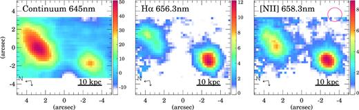
![SWIFT emission maps of the XMM2 system. The panels show rest-frame 645 nm continuum (left), H α 656.3 nm (middle), and [N ii]658.3 nm (right). The units for the continuum and emission line maps are 10−15 erg cm−2 s−1 $\mu$m−1 and 10−17 erg cm−2 s−1, respectively. The scale represents 10 kpc at the distance of the system. The red circle in the right-hand panel corresponds to the seeing FWHM. The two arrows in the lower left-hand corner indicate the North and East directions on the maps.](https://oup.silverchair-cdn.com/oup/backfile/Content_public/Journal/mnras/486/4/10.1093_mnras_stz1218/1/m_stz1218fig2.jpeg?Expires=1750306014&Signature=KMyQBAbaMi6CafluPMGOIw40wLG0-4tJfFnwzFjhN9phzpyvd3ezNCzcSzQujztDpnOXF4~GCuS2zPJP2dboh2CRkYXyGC0k17mGLRksl-2BmqAQ9iR-rdbw0t-O-TC8B9GYLCRZdNDEEsHpGJAU6czrdpRN0FVvbkEC6JdYIDac86tBnA3daCe2JTh~-0tKyjvufy0JYNbhBqitiETSg7UNbGXZJNbrrecSnlMw4BTL9J04mmQccjH5-Hcq1tUotpKppv9iSaFTot3ZGjc~EqlrMZA9SHDWM93aZZ1VOrfHwb3l6HLU59sjWpJGjHPup4VlZzTyAia1hCYG1ZEdtw__&Key-Pair-Id=APKAIE5G5CRDK6RD3PGA)
SWIFT emission maps of the XMM2 system. The panels show rest-frame 645 nm continuum (left), H α 656.3 nm (middle), and [N ii]658.3 nm (right). The units for the continuum and emission line maps are 10−15 erg cm−2 s−1 |$\mu$|m−1 and 10−17 erg cm−2 s−1, respectively. The scale represents 10 kpc at the distance of the system. The red circle in the right-hand panel corresponds to the seeing FWHM. The two arrows in the lower left-hand corner indicate the North and East directions on the maps.
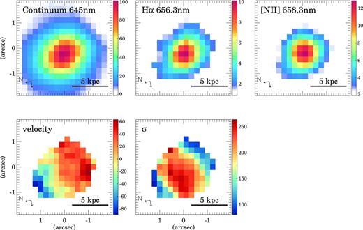
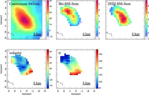
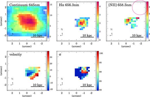
![SWIFT emission maps of XMM2 W. The top panels show rest-frame 645 nm continuum (left), H α 656.3 nm (middle), and [N ii]658.3 nm (right). The units for the continuum and emission line maps are 10−15 erg cm−2 s−1 $\mu$m−1 and 10−17 erg cm−2 s−1, respectively. The bottom panels show the velocity field (left) with respect to the systemic velocity (see Table 1) and the velocity dispersion σ (right). Both velocity maps are in km s−1. The scale represents 5 kpc at the distance of the galaxy. The two arrows in the lower left-hand corner indicate the North and East directions on the maps.](https://oup.silverchair-cdn.com/oup/backfile/Content_public/Journal/mnras/486/4/10.1093_mnras_stz1218/1/m_stz1218fig3.jpeg?Expires=1750306014&Signature=xAXSvFujnZBDoltSFXi4asWhlihxfNEX3yvV3MSW6f9OYAAsxFvib~8-XpuZEST2ciZasHF1n33vI-8nqcVnWxhR2K0Bw51NVW9skpUm-1jBzt8JtPeRwtIcV5c1--dr4MCzXtZlr-dnkWBdd4r~psDGgtk~KTLPqxTk0-XudWDwjuTrJhi9B9bEbPm1ifS8bTlvl7napQCfKx3V4P0cPkjDTrQ8BInNuertp6BovoT6o9-qd6mPKu~KmZUP9pzBkhFwavNK5tinqOIY3DeWcmhjUcEpRSbGJSgNuZZwlayS0LvoDEbtTA0aSFcDD3x1rDPF7ennon968nerfpm9Fg__&Key-Pair-Id=APKAIE5G5CRDK6RD3PGA)
SWIFT emission maps of XMM2 W. The top panels show rest-frame 645 nm continuum (left), H α 656.3 nm (middle), and [N ii]658.3 nm (right). The units for the continuum and emission line maps are 10−15 erg cm−2 s−1 |$\mu$|m−1 and 10−17 erg cm−2 s−1, respectively. The bottom panels show the velocity field (left) with respect to the systemic velocity (see Table 1) and the velocity dispersion σ (right). Both velocity maps are in km s−1. The scale represents 5 kpc at the distance of the galaxy. The two arrows in the lower left-hand corner indicate the North and East directions on the maps.
For the kinematic analysis in Section 3.3, we use the individual maps presented in Fig. 2 and Appendix A. These emission line and kinematic maps have been clipped to a SNR > 5 to exclude noisy spaxels from the modelling.
3.2 Integrated spectra
We extracted the integrated spectra of the individual objects in our sample by adding those spaxels where any emission line is detected at more than three times the standard deviation of the continuum. Similar to the spatially resolved analysis, we fitted a model consisting of a linear function for the stellar continuum and three Gaussian profiles with the same constraints described in Section 3.1. For BOOTES1 and SWIRE3, we added three broad Gaussian profiles to account for the broad profiles observed in their integrated spectra. We note, that the SWIRE3 emission line is dominated by the broad component. Therefore, the narrow component is not detected in the individual spaxels and it is only apparent in the higher SNR-integrated spectrum.
The results of the fits are presented in Tables 2 and 4 for the galaxies with narrow and narrow plus broad line profiles, respectively. We show the observed spectra and the best-fitting models in Fig. 4.
![SWIFT-integrated spectra around the redshifted H α emission line for the individual objects (the black histogram). The best-fitting model is indicated by the red solid line. For BOOTES1 and SWIRE3, the best-fitting model includes the narrow (the green line) and broad (the blue line) Gaussian profiles for the H α and [N ii] emissions.](https://oup.silverchair-cdn.com/oup/backfile/Content_public/Journal/mnras/486/4/10.1093_mnras_stz1218/1/m_stz1218fig4.jpeg?Expires=1750306014&Signature=kIqUUSY-RIez38mmmiszrPb6vQXVLXRgXBTVugyUJudPLgaIpc-FVDmCc-Z6dt9kmLEHOeQv9ZjdqyRxMD3WOsgYrrQIrA1936LEkqcvg6IAF9rBh2IxmqTkdCjH7aFGSppuAcUGcJbzTse35GP49AV5jrRYWoj797jiYRKC5Vj-7zv6wjmDQ0VZySdsBU67baiSPWgrBY63CMZGTuSn9BdkABQf1CiRjY7ihCXy96-BW7nUHDldkcExKviGEKcpTsBSaorhfLJ6UxuqBsC8Bki4u7TYbLKynUOheDlAdSrhV8bWdHs~HEFYhjUoGS6z0PuTob312hCjUthh666iYA__&Key-Pair-Id=APKAIE5G5CRDK6RD3PGA)
SWIFT-integrated spectra around the redshifted H α emission line for the individual objects (the black histogram). The best-fitting model is indicated by the red solid line. For BOOTES1 and SWIRE3, the best-fitting model includes the narrow (the green line) and broad (the blue line) Gaussian profiles for the H α and [N ii] emissions.
H α and [N ii]658.3 nm emission properties.
| Name | λH αa | F(H α)b | |$\frac{\rm [NII]658.3\, nm}{\rm H\alpha }$| c | vd | σ e | L(H α)f | SFR(H α)g |
|---|---|---|---|---|---|---|---|
| (nm) | (10−16 erg cm−2 s−1) | (km s−1) | (km s−1) | (1040 erg s−1) | (M⊙ yr−1) | ||
| XMM2 W | 786.9 ± 0.9 | 9.22 ± 0.33 | 2.26 ± 0.09 | 53817 ± 63 | 191 ± 53 | 10.5 | 0.56 |
| XMM2 E | 787.4 ± 1.3 | 5.10 ± 0.17 | 1.41 ± 0.06 | 54004 ± 91 | 192 ± 78 | 5.8 | 0.31 |
| CDFS2 N | 819.2 ± 0.6 | 9.15 ± 0.21 | 1.16 ± 0.03 | 65409 ± 48 | 159 ± 71 | 17.1 | 0.92 |
| CDFS2 S | 819.2 ± 0.2 | 7.29 ± 0.04 | 0.71 ± 0.01 | 65402 ± 12 | 129 ± 50 | 13.6 | 0.73 |
| CDFS1 W | 845.9 ± 0.8 | 2.68 ± 0.12 | 2.05 ± 0.10 | 74483 ± 69 | 163 ± 51 | 7.1 | 0.38 |
| CDFS1 E | 847.2 ± 0.1 | 4.79 ± 0.02 | 0.39 ± 0.01 | 74915 ± 6 | 90 ± 11 | 12.9 | 0.69 |
| SWIRE5 Wh | 784.4 ± 0.9 | 0.64 ± 0.03 | 0.72 ± 0.05 | 52896 ± 60 | 80 ± 2 | 0.7 | 0.04 |
| SWIRE5 E | 896.7 ± 0.4 | 50.13 ± 0.48 | 0.58 ± 0.01 | 90655 ± 39 | 204 ± 37 | 230.2 | 12.36 |
| SWIRE7 | 927.8 ± 0.2 | 3.73 ± 0.05 | ⋅⋅⋅ | 99839 ± 19 | 80 ± 2 | 22.8 | 1.23 |
| BOOTES2 | 819.7 ± 1.8 | 8.74 ± 0.45 | 2.24 ± 0.13 | 65560 ± 140 | 237 ± 98 | 16.4 | 0.88 |
| FLS02 N | 942.5 ± 0.2 | 3.76 ± 0.03 | 0.90 ± 0.01 | 104004 ± 17 | 152 ± 74 | 26.1 | 1.40 |
| FLS02 S | 942.9 ± 0.1 | 1.55 ± 0.01 | 0.71 ± 0.01 | 104118 ± 15 | 135 ± 56 | 10.8 | 0.58 |
aObserved wavelength of the H α transition.
bObserved H α flux.
cObserved [NII]658.3 nm/H α ratio.
dVelocity derived from the H α and [NII]658.3 nm emission using the relativistic velocity definition.
eWidth of the best-fitting Gaussian profiles.
fObserved H α luminosity.
gSFR derived from the observed H α luminosity using the Murphy et al. (2011) calibration.
hSWIRE5 W is a foreground galaxy not related to the ULIRG SWIRE5 E (see Table 1).
3.3 Kinematic models
To analyse the kinematic information in the data cubes, we used galpak3D (Bouché et al. 2015). This software takes the observed data cube as input and, using a Bayesian approach, produces a best-fitting rotating disc model. To determine the best-fitting parameters, galpak3D convolves the model with both the point spread function (Table 1) and the spectral line spread function (about 80 km s−1). Doing so, it is possible to recover the intrinsic velocity dispersion and amplitude of the rotation curve even when the galaxies are just marginally spatially resolved like in our case.
For the rotating disc model, we assume that the H α emission intensity in these galaxies follows a 2D Gaussian distribution, which the rotation curve can be modelled with an arctan functional form, and that the intrinsic velocity dispersion (σ) is spatially constant in the disc (see Bouché et al. 2015 for details). Then, galpak3D finds the spatial parameters (radius, inclination, and position angle) for the 2D Gaussian intensity distribution as well as the kinematic parameters (intrinsic velocity dispersion, systemic velocity, turnover radius, and maximum velocity) for the arctan model.
We show the best-fitting models in Figs 5 and C1-C7 in Appendix C. These models can reproduce the observed flux with residuals lower than 10–20 per cent for most of the galaxies. For the velocity fields, the typical residual is lower than 20 km s−1. For the σ maps, the residuals are also about 20 km s−1. The best-fitting parameters are listed in Table 3.
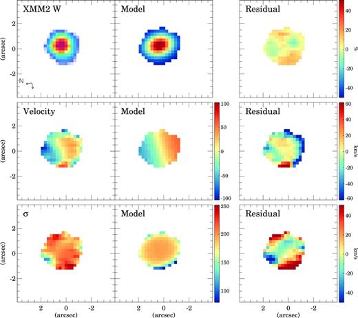
galpak3D model of XMM2 W. The first column shows the observed flux, velocity, and velocity dispersion (σ). The second column is the best-fitting model, and the third column the residuals. The velocity and σ panels are in km s−1 units. The residual flux map shows the difference between the observed and the model in percentage. The two arrows in the lower left-hand corner indicate the North and East directions on the maps.
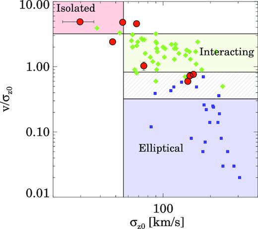
Ratio between the amplitude of the rotation curve and the velocity dispersion for the SWIFT intermediate-z U/LIRGs (the red circles), local U/LIRGs with |$\log L_{\rm IR}\,/\, L_\odot\,\, \gt\,\, 11.6$| (the green diamonds; García-Marín et al. 2009; Bellocchi et al. 2013), and local ellipticals (the blue squares; Cappellari et al. 2007). The observed velocity dispersions of the intermediate-z U/LIRGs have been corrected to account for the expected increase of the velocity dispersion with z (see Section 4.1). The red, green, and blue shaded areas indicate the typical ratios observed in isolated, interacting, and elliptical objects. The area filled with the green and blue lines indicates a range a ratios common for both interacting and elliptical galaxies (see Section 4.1).
Parameters of the best-fitting galpak3D model.
| Name | i a | PA b | R c | vmax d | σ e | v/σ f | |$\frac{f_{\rm gas}({\rm z = 0)}}{f_{\rm gas}({\rm z = z_{\rm U\,/\, LIRG}})}$| g | |$\sigma _{\rm z_0}$| h |
|---|---|---|---|---|---|---|---|---|
| (deg) | (deg) | (arcsec kpc−1) | (km s−1) | (km s−1) | (km s−1) | |||
| XMM2 W | 62 | 5 | 0.66/2.2 | 86 ± 9 | 195 ± 10 | 0.44 ± 0.05 | 0.73 | 142 |
| XMM2 E | 35 | 26 | 0.41/1.4 | 119 ± 10 | 212 ± 15 | 0.56 ± 0.06 | 0.73 | 155 |
| CDFS2 S | 46 | −48 | 0.61/2.4 | 78 ± 16 | 109 ± 8 | 0.72 ± 0.16 | 0.69 | 75 |
| CDFS1 W | 67 | 125 | 2.58/11 | 265 ± 9 | 84 ± 5 | 3.15 ± 0.22 | 0.65 | 55 |
| CDFS1 E | 48 | −49 | 0.82/3.6 | 115 ± 6 | 74 ± 6 | 1.55 ± 0.15 | 0.65 | 48 |
| SWIRE5 E | 37 | 19 | 0.92/4.7 | 310 ± 11 | 114 ± 9 | 2.72 ± 0.24 | 0.60 | 68 |
| SWIRE7 | 30 | 51 | 0.48/2.7 | 144 ± 18 | 52 ± 8 | 2.77 ± 0.55 | 0.53 | 76 |
| BOOTES2 | 44 | 47 | 0.80/3.1 | 108 ± 7 | 215 ± 12 | 0.50 ± 0.04 | 0.69 | 148 |
aGalaxy inclination.
bPosition angle (East of North) of the blue-shifted part of the kinematic major axis.
cFWHM/2 of the 2D Gaussian spatial model in angular and linear units at the distance of the each object.
dDe-projected semi-amplitude of the rotation curve.
eIntrinsic velocity dispersion of the discs. This model assumes that the velocity dispersion is uniform within the disc.
fDynamical ratio between the de-projected velocity semi-amplitude and the intrinsic velocity dispersion.
H α and [N ii]658.3 nm emission properties in galaxies with a broad component.
| Name | λH α a | F(H αnarrow)b | |$\frac{\rm H\alpha _{\rm broad}}{\rm H\alpha _{\rm narrow}}$| c | |$\frac{\rm [NII]658.3\, nm}{\rm H\alpha _{\rm narrow}}$| d | |$\frac{\rm [NII]658.3\, nm}{\rm H\alpha _{\rm broad}}$| e | vnarrow f | vbroad g | σnarrow h | σbroad i | L(H αnarrow) j |
|---|---|---|---|---|---|---|---|---|---|---|
| (nm) | (10−16 erg cm−2 s−1) | (km s−1) | (km s−1) | (km s−1) | (km s−1) | (1040 erg s−1) | ||||
| SWIRE3 | 752.7 ± 0.8 | 11.50 ± 0.53 | 12.49 ± 0.58 | 0.87 ± 0.06 | 0.77 ± 0.01 | 40835 ± 44 | 41039 ± 51 | 71 ± 53 | 313 ± 80 | 6.7 |
| BOOTES1 | 886.8 ± 0.3 | 7.40 ± 0.13 | 1.77 ± 0.05 | 0.90 ± 0.02 | 2.80 ± 0.07 | 87614 ± 26 | 87507 ± 64 | 96 ± 34 | 377 ± 72 | 30.8 |
aObserved wavelength of the narrow H α transition.
bObserved flux of the narrow H α component.
cRatio between the broad and narrow H α fluxes.
d,eObserved [NII]658.3 nm/H α ratio for the narrow and broad components of these transitions, respectively.
f,gVelocity derived from the narrow and broad H α and [NII]658.3 nm emission using the relativistic velocity definition, respectively.
h,iWidth of the best-fitting Gaussian profiles for the narrow and broad components, respectively.
jObserved luminosity of the H α narrow component.
We excluded from the kinematic modelling CDFS2 N, SWIRE3, BOOTES1, FLS02 N, and FLS02 S, so in total we have modelled eight objects with galpak3d. For CDFS2 N, the emission map and the velocity field might be compatible with two counter-rotating interacting galaxies approximately along the East–West direction separated by ∼10 kpc (see Fig. B2). SWIRE3 and BOOTES1 have broad H α emission (see Fig. 4) so the narrow emission, associated with the disc rotation, is not well constrained. For FLS02 N, the H α emission seems to be spatially unresolved so no kinematic information is available from this transition (see Fig. B11), and FLS02 S contains too few spaxels with H α emission for a reliable modelling (see Fig. B12).
SDSS images are available for 7 of 9 systems in our sample. However, the limited angular resolution and sensitivity of these images is not sufficient to study the morphology of these objects, identify perturbed morphologies, or detect tidal tails. High angular resolution imaging of these system would be needed to firmly establish their actual morphology.
4 DISCUSSION
Magdis et al. (2014) found that intermediate-z (0.2 < z < 0.9) U/LIRGs have physical properties that differ from those of local U/LIRGs. Based on Herschel [C ii]158 |$\mu$|m and ground-based CO observations, these intermediate-z U/LIRGs present stronger [C ii] emission with respect to the total LIR and lower SFEs than local ULIRGs. To explain these differences, Magdis et al. (2014) proposed that the starbursts of these intermediate-z U/LIRGs are not driven by galaxy mergers and that, unlike local ULIRGs, they might take place in extended regions within the galaxy. Also, Magdis et al. (2014) suggested that the evolution of the metal content of the U/LIRGs at these intermediate-z might also explain the observed physical properties.
To investigate these possibilities, in this section, we compare the kinematics, SFR obscuration, metal abundances, and dust temperatures of local U/LIRGs and our sample of intermediate-z U/LIRGs.
4.1 Dynamical ratio
The dynamical ratio defined as the ratio between the velocity amplitude of the rotation curve and the velocity dispersion can be used to parametrize the kinematic state of a system (e.g. Epinat et al. 2010; Bellocchi et al. 2013). Objects that are rotationally supported (i.e. discs) have high |$v\,/\, \sigma$| ratios, whereas interacting and merging systems have higher velocity dispersions (σ) and therefore lower |$v\,/\, \sigma$| ratios.
For this comparison, we plot the dynamical ratio for the eight intermediate-z U/LIRGs whose gas kinematics were modelled with galpak3D (see Section 3.3) using the corrected |$\sigma _{\rm z_0}$| values. Galaxy pairs are considered individually in this Section. We also plot the dynamical ratios of local U/LIRGs with similar optical IFS data from García-Marín et al. (2009) and Bellocchi et al. (2013). We limit the local sample to galaxies with |$\log L_{\rm IR}\,/\, L_\odot \gt 11.6$| to match the luminosity range of the intermediate-z objects. From the dynamical ratios and velocity dispersions observed in isolated U/LIRGs (defined as class 0 objects in Bellocchi et al. 2013), we determine a threshold value to separate isolated and interacting galaxies as the mean value of isolated objects plus (minus) three times the standard deviation of the velocity dispersion (dynamical ratio). These threshold values are σ < 56 km s−1 and v|$\,/\, \sigma \,\,\gt\,\, 3.2$|. We also compare with the velocity dispersions and dynamical ratios of local elliptical galaxies from Cappellari et al. 2007. Similarly, the threshold between interacting and elliptical is calculated using the mean dynamical ratio plus /minus three times its standard deviation. We note that dynamical ratios between 0.3 and 0.8 are observed in both elliptical and interacting systems.
Using the criteria described above, we find that half, 4 of 8, of the SWIFT intermediate-z U/LIRGs are compatible with the kinematic parameters measured in interacting systems and elliptical galaxies. Three of these objects belong to systems with various galaxies (CDFS2 S,1 XMM2 E, and W). For the fourth object, BOOTES2, the continuum image suggests that it is an isolated object. This might indicate a more advanced phase of the interaction where the separation between the two nuclei is not resolved by the SWIFT data (5.5 kpc spatial resolution for this object). CDFS1 W and SWIRE7 lie in the region of isolated systems, so they might actually be isolated galaxies (SWIRE7) or be at an early stage of the interaction (CDFS1 W). Finally, two objects (SWIRE5 E and CDFS1 E) have intermediate dynamical ratios and velocity dispersions. This diagram suggests that some fraction (1–2 of 8) of the intermediate-z U/LIRGs (0.2 < z < 0.4) are isolated discs.
4.2 Obscured star formation
SF in local interacting U/LIRG usually occurs in compact (r < 1 kpc) nuclear regions (e.g. Rujopakarn et al. 2011; Arribas et al. 2012). These compact starbursts are heavily affected by dust extinction (e.g. Rigopoulou et al. 1999; Piqueras López et al. 2013) and the SFRs derived from the optical H α emission can be a few orders of magnitude lower than those derived from IR tracers (e.g. Hopkins et al. 2001; Dopita et al. 2002; Rodríguez-Zaurín et al. 2011).
By contrast, higher redshift (z > 1−3) U/LIRGs have more extended SF (r > 2 kpc; e.g. Iono et al. 2009; Simpson et al. 2015; Rujopakarn et al. 2016) and are less affected by dust extinction (e.g. Buat et al. 2015).
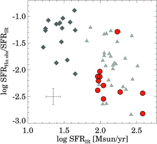
Ratio between the SFR from the observed H α emission (not corrected for extinction) and the IR SFR as a function of the IR SFR. The red circles correspond to the SWIFT intermediate-z U/LIRGs and the grey triangles to local U/LIRGs (|$\log L_{\rm IR}\,/\, L_\odot \,\,\gt\,\, 11.6$|) from Rodríguez-Zaurín et al. (2011). The dark grey diamonds correspond to lower luminosity LIRGs also from Rodríguez-Zaurín et al. (2011). The average uncertainties are indicated by the error bars at the bottom left-hand corner.
The SFRH α/SFRIR ratio is a proxy for the average obscuration of the SF, assuming a constant SFR during the last ∼100 Myr since H α is only sensitive to the less obscured SF, while the IR luminosity traces the obscured SF (see e.g. Kennicutt & Evans 2012). For comparison, we plot the same ratio for the sample of local U/LIRGs of Rodríguez-Zaurín et al. (2011) scaled to the Murphy et al. (2011) SFR calibrations.
The average log SFRH α/SFRIR ratio of our intermediate-z U/LIRGs is −2.2 ± 0.4, while this ratio is −1.9 ± 0.4 for local U/LIRGs. Therefore, our intermediate-z U/LIRGs have average dust extinctions slightly higher than those of local U/LIRGs for the same LIR but within the scatter observed in local objects. Therefore, we do not find evidence for the expected decrease of the dust extinction in these intermediate-z U/LIRGs. This suggests that the SF taking place in these intermediate-z galaxies resembles the SF of local U/LIRGs in terms of obscuration. To fully confirm that the SF in local and intermediate-z U/LIRGs is similar, we will need direct measurements of the size of the SF regions through high-angular resolution data.
4.3 Metallicity
In this section, we use the [N ii]658nm/H α ratio (N2 index) to compare the metalicity of the SWIFT U/LIRGs and that of local U/LIRGs. The N2 index is well correlated with the metal abundance of galaxies (e.g. Pettini & Pagel 2004; Marino et al. 2013). However, this optical index may be subject to extinction effects, specially in dusty systems such as U/LIRGs. Pereira-Santaella et al. (2017) used far-IR metallicity diagnostics, which are not affected by dust extinction, and found that, for local ULIRGs, optical and far-IR metallicity diagnostics provide compatible results. Therefore, the results presented in this section should not be sensitive to the obscuration on these systems.
We plot the N2 index in Fig. 8 as a function of the IR luminosity for the SWIFT U/LIRGs and for local U/LIRGs from Rupke, Veilleux & Baker (2008), Alonso-Herrero et al. (2009), and Monreal-Ibero et al. (2010). SWIFT sources with broad emission lines (i.e. AGN) are excluded from this plot. We find that the SWIFT U/LIRGs have N2 indexes (1.1 ± 0.8) slightly higher than local U/LIRGs (0.7 ± 0.3). However, this difference is not statistically significant.
![[N ii]658nm/H α ratio (N2 index) as a function the IR luminosity for the SWIFT U/LIRGs (the red circles) and for local U/LIRGs (the grey triangles $\log L_{\rm IR}\,/\, L_\odot \,\,\gt\,\, 11.6$; and the dark grey diamonds $\log L_{\rm IR}\,/\, L_\odot\,\, \lt\,\, 11.6$). The data for the local U/LIRGs are from Rupke et al. (2008), Alonso-Herrero et al. (2009), and Monreal-Ibero et al. (2010). The solid grey line marks the mean N2 index for local U/LIRGs and the dashed line its ±1σ confidence range. The two SWIFT U/LIRGs with broad H α profiles (SWIRE3 and BOOTES1) are not included in this figure. The average uncertainties are indicated by the error bars at the top left-hand corner.](https://oup.silverchair-cdn.com/oup/backfile/Content_public/Journal/mnras/486/4/10.1093_mnras_stz1218/1/m_stz1218fig8.jpeg?Expires=1750306014&Signature=nPEcmQiRyj-zv3nVJzNzFjh0cEl4Sc3fpaT5mN7wC9ka3tJYjAgIiledd4YvwaTdXyl~tYGvheB8aG5MiBq0pfSHimcKM1ph61hSVCUfmFdurVbYJ1Ng~EgX0DVAZha-TwkH-lXPdpLL7svCWMcFfNIZqTPEATqU5zh~XFdVZ0TuG92FHbJs62dHVn4szCN4fuAEiSNmMlf1dpcWve7KcgWpW8LZ6LwbF1vBWVoJmfsra5VFQkxeT6K-tJDj2iGkA071~LczeiaNI3KkuGWbBhp0amrMr~KwPBE3XGx4Jj9dpYyapVbIYxQ1N52R-1l7iRuY7tHSwoZFKBY2PEJfgw__&Key-Pair-Id=APKAIE5G5CRDK6RD3PGA)
[N ii]658nm/H α ratio (N2 index) as a function the IR luminosity for the SWIFT U/LIRGs (the red circles) and for local U/LIRGs (the grey triangles |$\log L_{\rm IR}\,/\, L_\odot \,\,\gt\,\, 11.6$|; and the dark grey diamonds |$\log L_{\rm IR}\,/\, L_\odot\,\, \lt\,\, 11.6$|). The data for the local U/LIRGs are from Rupke et al. (2008), Alonso-Herrero et al. (2009), and Monreal-Ibero et al. (2010). The solid grey line marks the mean N2 index for local U/LIRGs and the dashed line its ±1σ confidence range. The two SWIFT U/LIRGs with broad H α profiles (SWIRE3 and BOOTES1) are not included in this figure. The average uncertainties are indicated by the error bars at the top left-hand corner.
4.4 Dust temperature
The sample of intermediate-z U/LIRGs studied in this work was selected based on their observed 250 |$\mu$|m flux. This wavelength is considerably longer than the 60 |$\mu$|m flux used for the selection of U/LIRGs both locally (Kim & Sanders 1998) and at intermediate-z (Combes et al. 2011) based on IRAS observations. Therefore, the 250 |$\mu$|m selection might be more sensitive to selecting galaxies with colder dust than samples selected at shorter wavelengths.
To investigate this, we compare the L250/LIR ratio measured in our intermediate-z U/LIRGs and that of local U/LIRGs (Fig. 9). For the intermediate-z galaxies, we use the Herschel/SPIRE 250 |$\mu$|m fluxes from Magdis et al. (2014). For the local U/LIRGs, we take SPIRE 250 |$\mu$|m fluxes, distances, and LIR published by Chu et al. (2017). This includes most of the local U/LIRGs in the Revised Bright Galaxy Sample (Sanders et al. 2003). In addition, we obtained the SPIRE 250 |$\mu$|m fluxes for another 16 ULIRGs observed by Herschel (Sturm et al. 2011; Farrah et al. 2013) from the SPIRE Point Source Catalog (Schulz et al. 2017). A k-correction was applied to the observed 250 |$\mu$|m fluxes for all the galaxies assuming a dust temperature of 40 K. This correction varies <15 per cent for dust temperatures between 25 and 50 K and reduces the 250 |$\mu$|m fluxes by 15 per cent and 50 per cent on average for the local and the intermediate-z ULIRGs, respectively.
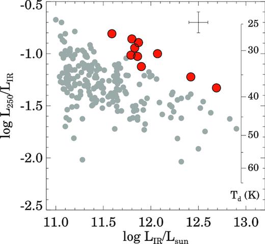
L250/LIR ratio as a function of the total IR luminosity (LIR). The red circles represent our sample of intermediate-z U/LIRGs. The grey circles correspond to local U/LIRGs from Chu et al. (2017), Sturm et al. (2011), and Farrah et al. (2013). The dust temperature (Td) scale is calculated assuming a grey body with β = 1.6 (see Section 4.4 for details). The average uncertainties are indicated by the error bars at the top right-hand corner.
The L250/LIR ratio is sensitive to the dust temperature. Assuming that the IR emission is well represented by a grey-body with β = 1.6 (Casey 2012), we calculated the L250/LIR ratio as a function of the dust temperature (see Fig. 9). We find that most of the U/LIRGs have ratios compatible with dust temperatures between 25 and 50 K. Also, we observe the known trend of increasing dust temperatures with increasing LIR (e.g. Hwang et al. 2010).
We find that these intermediate-z U/LIRGs have L250/LIR ratios higher than local U/LIRGs with the same LIR. This suggests that the average dust temperature in these systems is lower than in local U/LIRGs. Therefore, the selection of our sample at 250 |$\mu$|m reveals a population of cold intermediate-z U/LIRGs different from local U/LIRGs and warm intermediate-z U/LIRGs selected at 60 |$\mu$|m (Combes et al. 2011).
5 CONCLUSIONS
We compared the properties of a sample of nine intermediate-z (0.2 < z < 0.4) U/LIRG systems with those of local U/LIRGs using optical IFS data. We aim to determine if the differences between local U/LIRGs and z > 1 U/LIRGs are already present at 0.2 < z < 0.4. We used the H α + [N ii] emission to model the 2D kinematics and to measure the N2 metallicity index. These new results for the intermediate-z U/LIRGs, combined with their IR properties (LIR and L250 |$\mu$|m), were used to compare the dynamical state, SFR obscuration, metallicity, and dust temperature of local and intermediate-z U/LIRGs. The main results of this paper are the following:
The optical IFS data reveal that 4 of 9 U/LIRGs are composed by two individual objects located at projected distances between 20 and 30 kpc. Therefore, they are at an early stage of the interaction. The remaining five objects in our sample appear as isolated galaxies. However, higher angular resolution imaging is needed to identify, if present, signs of recent interaction/merger events in these five objects. In two systems, we find broad H α profiles σ = 300−400 km s−1 (FWHM∼750−900 km s−1) in their integrated spectra suggesting the presence of an AGN.
The corrected for redshift effects velocity dispersion (|$\sigma _{\rm z_0}$|) and dynamical ratio (|$v\,/\, \sigma _{\rm z_0}$|) of these intermediate-z U/LIRGs indicate that half of them (4 of 8) belong to interacting systems and 1 or 2 of 8 are compatible with being isolated galaxies. For most cases (6 of 8), this classification is in agreement with that obtained from the images.
The ratio between the obscured SFR traced by the IR luminosity and the un-obscured SFR traced by H α of the intermediate-z U/LIRGs is compatible with the range measured in local U/LIRGs with the same LIR. Therefore, the obscuration properties of the SF regions in intermediate-z U/LIRGs seem to be comparable to those of local U/LIRGs.
The average N2 metallicity index ([N ii]658nm/H α ratio) of the intermediate-z U/LIRGs is slightly higher (1.1 ± 0.8) than that of local U/LIRGs (0.7 ± 0.3), although this difference is not statistically significant.
We find that the ratio between the 250 |$\mu$|m luminosity and the total LIR of these intermediate-z U/LIRGs is higher than that of local U/LIRGs with the same LIR. This is compatible with reduced dust temperatures in these intermediate-z U/LIRGs compared to local U/LIRGs. This, together with the enhanced molecular gas content traced by their CO emission (see Magdis et al. 2014), suggests different ISM conditions in these intermediate-z and local U/LIRGs.
In summary, the main differences between these intermediate-z U/LIRGs and local U/LIRGs are (1) intermediate-z U/LIRGs seem to be at an earlier interaction stage and (2) the dust temperature is lower in these U/LIRGs selected at 250 |$\mu$|m. On the contrary, the obscuration level of the SFR seems to be similar in both local and these intermediate-z U/LIRGs.
SUPPORTING INFORMATION
supplement.zip
Please note: Oxford University Press is not responsible for the content or functionality of any supporting materials supplied by the authors. Any queries (other than missing material) should be directed to the corresponding author for the article.
ACKNOWLEDGEMENTS
We thank the anonymous referee for useful comments and suggestions. MPS and DR acknowledge support from STFC through grant ST/N000919/1. MPS, NT, FC, MT, and MR acknowledge support from STFC through grant ST/N002717/1.
Footnotes
CDFS2 N is not modelled with galpak3D since it shows a complex kinematics that does not resemble a rotating disc (see Section 3.3).
REFERENCES
APPENDIX A: SWIFT CLOSE PAIRS EMISSION MAPS
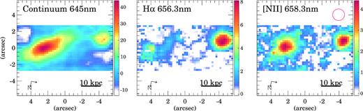
Same as Fig. 2 but for CDFS2.
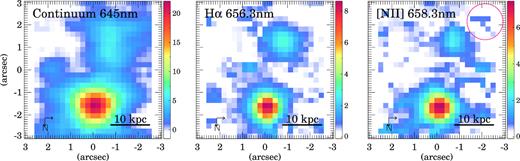
Same as Fig. 2 but for CDFS1.
Same as Fig. 2 but for FLS02.
APPENDIX B: SWIFT INDIVIDUAL EMISSION MAPS
Same as Fig. 3 but for XMM2 E.
Same as Fig. 3 but for CDFS2 N.
Same as Fig. 3 but for CDFS2 S.
Same as Fig. 3 but for CDFS1 W.

Same as Fig. 3 but for CDFS1 E.
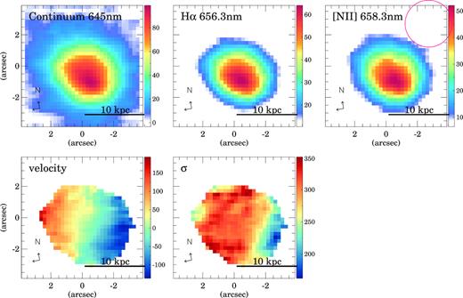
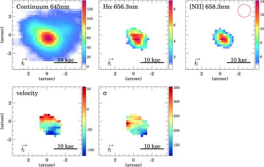
![Same as Fig. 3 but for SWIRE5. Note that the SWIRE5 W H α and [N ii] emission are not included in the maps because of the lower redshift of this component (0.195) compared to the redshift (0.366) of the main IR emitter of the system (SWIRE5 E). The red circle in the right-hand panel corresponds to the seeing FWHM.](https://oup.silverchair-cdn.com/oup/backfile/Content_public/Journal/mnras/486/4/10.1093_mnras_stz1218/1/m_stz1218figb6.jpeg?Expires=1750306014&Signature=nuZ-sPOr5Al2IQ1UyNVV4eS~Y6pZIaESegb7iWQTrf2vFTKvLHz5zwy7lB~r7jtuqfLAZDztdRBZjQtn1AroHsIoC7KqdMaCIgrtn-SZ1atQe9MWxcFQ8DtgrJL81jLj-TyZpCkXf6SuXGNN7naVmrwqtqCUcYpgwpogzbyZ~55Lz7r7ziqHwQSh4oelGb-qBc2ndzWLqvfbJcwjy6LbF3~ZQCZkTnUVCy6KtrA1B0kxOIHDWEQ6FtCRie5SQH3Gaeb8r2lx-vSpRyyZAaqD9Gp5wZMW40Flyz~3eB2fE5YsV8ENHJh68LaVzTNp3CfzQtC-V~MRoRiKXXkXR0tz0w__&Key-Pair-Id=APKAIE5G5CRDK6RD3PGA)
Same as Fig. 3 but for SWIRE5. Note that the SWIRE5 W H α and [N ii] emission are not included in the maps because of the lower redshift of this component (0.195) compared to the redshift (0.366) of the main IR emitter of the system (SWIRE5 E). The red circle in the right-hand panel corresponds to the seeing FWHM.
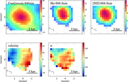
Same as Fig. 3 but for SWIRE3. The red circle in the right-hand panel corresponds to the seeing FWHM.
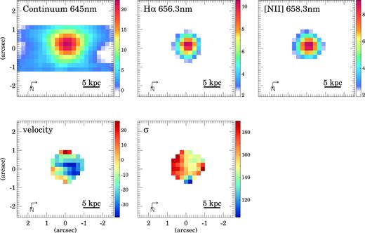
Same as Fig. 3 but for SWIRE7. The red circle in the right-hand panel corresponds to the seeing FWHM.
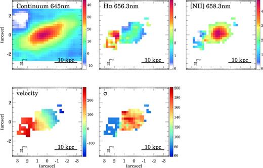
![Same as Fig. 3 but for BOOTES1. The velocity dispersion is not well constrained so this map is not included here. The lower panels also show the distribution of the broad H α (middle), and [N ii] (right) emissions. The red circle in the right-hand panel corresponds to the seeing FWHM.](https://oup.silverchair-cdn.com/oup/backfile/Content_public/Journal/mnras/486/4/10.1093_mnras_stz1218/1/m_stz1218figb9.jpeg?Expires=1750306014&Signature=HDeeLBwZA27wiJMKHj3Q34dHk-e2oxOYSMqXCZ9B2RgEHMKZA8eqRCjphKR451XVKIsoMyT7EQhtTVgc4wkgj5WWkftXWQ1-y17FBX2ro~ttc2xkHImlEbIBi3eQ4F3OCYcZI1ze3-fl6e4E2qiWuMcn8ueKadFxlYqEKOfSta17D2yXA0fLQ-~hBEAaU-iazzyOApQQ0vzNl6XyXIWckl4eqoQMwR7qqNaDD6O6H3my2kdUGdRX0f9Zr4dods2MQqwiVyF35ywq2IDqKjmQ-kIvJl6gMCaECoqTmW5A~waq65eyqW--G9xam9BL3GNnyp3q3RkYDEMnRCOyUYaq0w__&Key-Pair-Id=APKAIE5G5CRDK6RD3PGA)
Same as Fig. 3 but for BOOTES1. The velocity dispersion is not well constrained so this map is not included here. The lower panels also show the distribution of the broad H α (middle), and [N ii] (right) emissions. The red circle in the right-hand panel corresponds to the seeing FWHM.
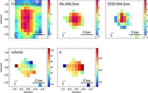
Same as Fig. 3 but for BOOTES2. The red circle in the right-hand panel corresponds to the seeing FWHM.
Same as Fig. 3 but for FLS02 N.
Same as Fig. 3 but for FLS02 S.
APPENDIX C: galpak3D MODELS
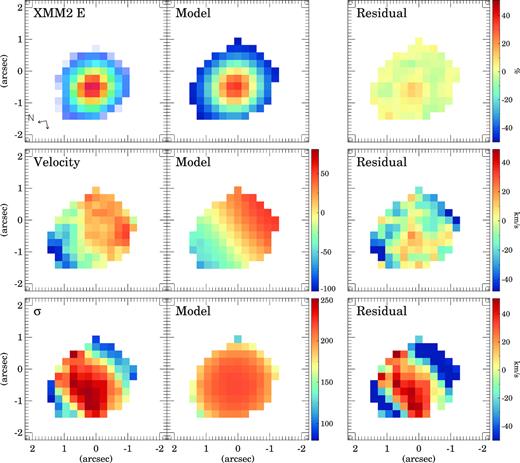
Same as Fig. 5 but for XMM2 E.
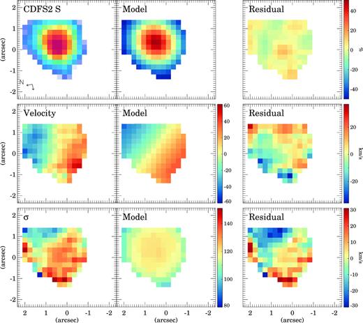
Same as Fig. 5 but for CDFS2 S.
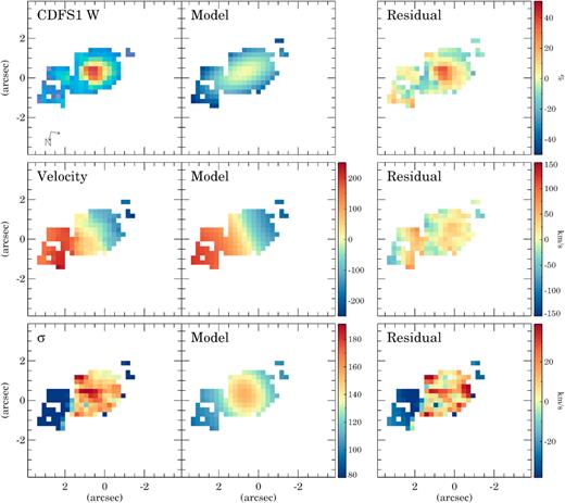
Same as Fig. 5 but for CDFS1 W.
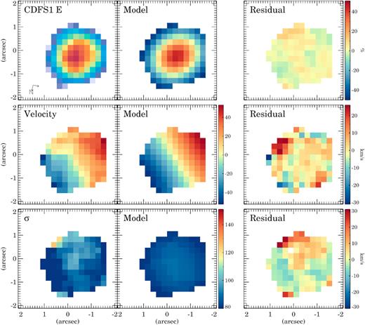
Same as Fig. 5 but for CDFS1 E.
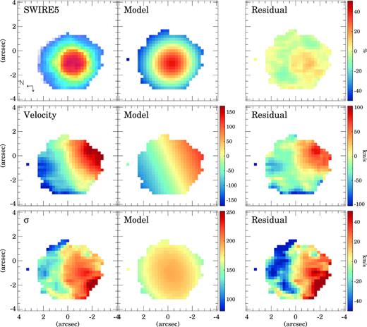
Same as Fig. 5 but for SWIRE5.
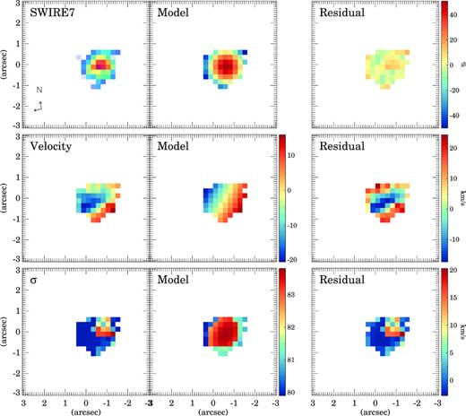
Same as Fig. 5 but for SWIRE7.
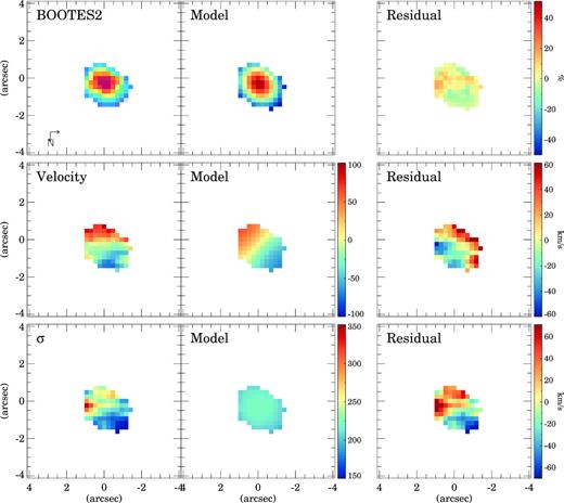
Same as Fig. 5 but for BOOTES2.
