


ABSTRACT
We use the cross-correlation between the thermal Sunyaev–Zeldovich (tSZ) signal measured by the Planck satellite and the luminous red galaxy (LRG) samples provided by the SDSS DR7 to study the properties of galaxy cluster and intra-cluster gas. We separate the samples into three redshift bins |$z_{1}=(0.16,\, 0.26)$|, |$z_{2}=(0.26,\, 0.36)$|, |$z_{3}=(0.36,\, 0.47)$|, and stack the Planck y-map against LRGs to derive the averaged y-profile for each redshift bin. We then fit the stacked profile with the theoretical prediction from the universal pressure profile (UPP) by using the Markov Chain Monte Carlo method. We find that the best-fitting values of the UPP parameters for the three bins are generally consistent with the previous studies, except for the noticeable evolution of the parameters in the three redshift bins. We simultaneously fit the data in the three redshift bins together, and find that the original UPP model cannot fit the data at small angular scales very well in the first and third redshift bins. The joint fits can be improved by including an additional parameter η to change the redshift dependence of the model (i.e. |$E(z)^{8/3}\, \rightarrow \, E(z)^{8/3+\eta }$|) with best-fitting value as |$\eta =-3.11^{+1.09}_{-1.13}$|. This suggests that the original UPP model with less redshift dependence may provide a better fit to the stacked tSZ profile.
1 INTRODUCTION
The clusters of galaxies are the important objects in learning the structure formation and cosmology in general. Around hot clusters, the gas is generally ionized with temperature above |$10^{6}\,$|K (McCarthy et al. 2007) and provides high density of hot electrons. The intra-cluster medium (ICM) can be studied by using direct X-ray imaging or the Sunyaev–Zeldovich effect (SZ effect; Sunyaev & Zeldovich 1972, 1980). Intensity of the former is proportional to the square of the electron density |${\sim } n^{2}_{\rm e}$| which could be sensitive to the centre baryons. In contrast, observation of the SZ effect depends on the integration of pressure profile, which could be used to trace down the gas distribution in the lower density region. These regions, such as filament, sheets and voids, are the locations believed to host most of the baryons (Haider et al. 2016; Tanimura et al. 2019a). For this reason, there has been a growing interest in predicting and measuring the SZ effect by using various techniques in microwave and radio bands (Birkinshaw & Gull 1978; Birkinshaw 1999; Carlstrom, Holder & Reese 2002; Ma et al. 2015).
One the other hand, by accurately measuring the Compton y-parameter, a more precise modelling of the pressure profile can be obtained. In 2010, Arnaud et al. (2010) investigated the cluster pressure profile with 33 local (z < 0.2) samples of clusters drawn from REXCESS catalogue observed by XMM–Newton. These samples span the mass range of 1014M⊙ < M500 < 1015M⊙ where the M500 is the mass of the centre of cluster within the radius of density equal to 500ρcrit. Arnaud et al. (2010) proposed the universal pressure profile (UPP) for the clusters and determined the parameter values by using the 33 massive clusters. Following Arnaud et al. (2010), Planck Collaboration V (2013) used the Planck’s 14-month nominal survey and 62 massive nearby clusters, and re-investigated the cluster UPP, and refined the parameter values. Besides these observational probes, Le Brun, McCarthy & Melin (2015) used the cosmo-OWLS simulation and tested the UPP against different AGN models, and refined the UPP model parameters.
In these studies, the tSZ effect is a very useful tool to explore the high-redshift galaxy clusters. Because the signal y is expected to be nearly independent of the redshift, the effect does not diminish with the increasing redshift. Therefore, the effect is very suitable for finding high-redshift clusters (Planck Collaboration VIII 2011) and cross-correlation with other large-scale structure tracers [e.g. cross-correlation with weak-lensing measurement (Ma et al. 2015; Hojjati et al. 2017)]. In addition, luminous red galaxies (LRGs) are early-type massive galaxies consisting mainly of old stars with little ongoing star formation. Thus LRGs are good tracers of galaxy clusters and underlying dark-matter distribution, and should be correlated with thermal SZ signal (Hoshino et al. 2015).
In this work, we will study this cross-correlation and explore the UPP of clusters. Since the Sloan Digital Sky Survey (SDSS) released its data, there have been increasingly large LRG catalogues that span more orders of magnitude in mass and occupy different distances. The samples we use here are DR7 LRG samples, which have mass range to 3 × 10¹² to 3 × 10¹⁴ M⊙ and redshift range of 0.16 < z < 0.47, and significantly overlap with the Planck all-sky Compton y-map. Therefore, providing the stacking results of the LRG samples at cosmological distances and fitting the UPP model is the main aim of this paper. We will provide robust tests of the UPP model parameters by this large LRG sample from SDSS DR7.
This paper is organized as follows. In Section 2, we present the Planck y-maps from the CMB and LRG catalogues from SDSS-DR7 used in this study, and the stacking results of LRG y-profile. In Section 3, we present the modelling of the stacked profiles by calculating the one-halo and two-halo terms of the stacked profile. In Section 4, we discuss the data analysis procedure and χ2 study in our work. In Section 5, we present the results of our numerical fitting and compare our results with other works. The summary and discussion are presented in the last section.
Throughout this paper, we adopt a spatially flat fiducial ΛCDM cosmology with Planck cosmological parameter values (Planck Collaboration XVI 2014), which are the fractional baryon density Ωb = 0.0490, fractional matter density Ωm = 0.3175, spectral index ns = 0.9624, rms matter fluctuation amplitude σ8 = 0.834, and h = 0.6711 defined as |$H_{0}=100\, h\, {\rm km}\, {\rm s}^{-1}\, {\rm Mpc}^{-1}$|, where H0 is the Hubble constant. We note that our constraint results are not very sensitive to the current determined values of cosmological parameters.
2 DATA
We adopt the same data sets used in Tanimura et al. (2019b) in our analysis: the LRG catalogue from the Sloan Digital Sky Survey seventh data release Kazin et al. (2010) and the Planck Compton y-map (Planck Collaboration XXII 2016) from the 2015 data release (Planck Collaboration I 2016). Each data is described briefly in this section.
2.1 LRG catalogue
LRGs are early-type, massive galaxies with little ongoing star formation, which are selected based on magnitude and colour cut. They are typically located in the centres of galaxy groups and clusters and have been used to detect and characterize the remnants of baryon acoustic oscillations at low to intermediate redshift (Eisenstein et al. 2005; Kazin et al. 2010; Anderson et al. 2014). The SDSS DR7 LRGs are selected in Kazin et al. (2010) and cover ∼20 per cent of the sky with almost a flat distribution. The LRG catalogue provides 105 831 LRGs with galaxy positions, magnitudes, and spectroscopic redshifts. Stellar masses of the LRGs are estimated in the New York University Value-Added catalogue (NYU-VAGC)1 using the K-correct software2 of Blanton & Roweis (2007) based on a stellar initial mass function of Chabrier (2003) and stellar evolution synthesis models of Bruzual & Charlot (2005). They are given in unit of h−2M⊙ and we adopt h = 0.6711 (Planck Collaboration XVI 2014).
Since not all LRGs are located in the centres of galaxy clusters, some LRGs may reside in them as ‘satellite’ galaxies. To minimize the satellite LRGs in our sample, we select locally (geometrically) most-massive LRGs (based on stellar mass) using a criterion that is analogous to that used in Planck Collaboration XI (2013): we remove a galaxy if a more massive galaxy resides within a tangential distance of 1.0 Mpc and within a radial velocity difference of |cΔz| < 1000 km s−1. After this selection, 101 407 locally most-massive LRGs are left that are likely to be ‘central’ LRGs. The detail of the sample is described in Tanimura et al. (2019b).
2.2 Planck y-map
The Planck tSZ map from the Planck 2015 data release is provided in HEALPix format (Gorski et al. 2005) 3 with a pixel resolution of Nside = 2048. Two types of algorithms, MILCA (Hurier, Macias-Perez & Hildebrandt 2013) and NILC (Remazeilles, Aghanim & Douspis 2013), are applied for the Planck band maps to extract the tSZ signal. They are based on ILC (internal linear combination) techniques aiming to preserve an astrophysical component for which the electromagnetic spectrum is known (Bennett et al. 2003). Our analysis is based on the MILCAy-map, but we find consistent results with the NILCy-map.
The 2015 data release also provides sky masks suitable for analysing the y-maps. The mask covers a point-source mask and galactic masks that exclude 40 per cent, 50 per cent, 60 per cent, and 70 per cent of the sky. We combine the point source mask with the 40 per cent galactic mask, which excludes ∼50 per cent of the sky. The mask is used in our stacking process such that for a given LRG, masked pixels in the y-map near that LRG are not accumulated in the stacked image. Since the mask may bias the y-profile, we accept 74 681 LRGs, for which ≥80 per cent of the region within a 40 arcmin circle around each LRG is available.
2.3 Stacking y-map centred on LRGs
We describe our procedure for stacking the Planck y-map at the positions of LRGs. We set a two-dimensional (2D) angular coordinate system of −40 arcmin < Δl < 40 arcmin and −40 arcmin < Δb < 40 arcmin, divided in 80 × 80 bins. For each LRG in the catalogue, we place it at the centre of the coordinate and subtract its local background signal of the mean tSZ signal in the annular region between 30 and 40 arcmin. This procedure nulls a large scale mode of fluctuation in the y-map, not due to the target object. We repeat this procedure for our sample of LRGs, stack them and finally divide the stack by the number of our sample.
In order to investigate a redshift evolution of tSZ signal (evolution of pressure profile), we divide our LRG sample into three redshift bins of sub-samples, z1 bin (0.16 < z < 0.26), z2 bin (0.26 < z < 0.36), and z3 bin (0.36 < z < 0.47). These redshift bins are selected to have an equal interval in redshift to probe the redshift evolution of pressure profiles around z ∼ 0.2, 0.3, and 0.4. The number of LRGs in each redshift bin is 18 083 in z1 bin, 29 586 in z2 bin, and 27 012 LRGs in z3 bin.
To study the redshift evolution of pressure profile, the effect due to differences of the mass distributions in different redshift bins (see Fig. 1) must be removed, and it needs to be probed by comparing the y-profiles with the ‘same’ mass distribution. The original mass distributions of LRG haloes at the three redshift bins are shown in Fig. 1 in halo mass (M500), for which halo masses are estimated by the stellar-to-halo mass relation in Wang et al. (2016) obtained from gravitational lensing measurements. Tanimura et al. (2019b) shows the y-profile of the LRGs can be described using this stellar-to-halo relation. We find that our constraint results are not quite sensitive to the stellar-to-halo relation. To obtain the same mass distributions in the three redshift bins, we find and select the minimum number of LRGs in a mass bin in the three z-bins (or the overlapped region of the three mass distributions, see Fig. 1), and adopt these LRGs as our sub-sample used in the following discussion. The derived mass distribution for the three z-bins is shown as hatched area in Fig. 1 and it provides 11 660 LRGs for each redshift bin.
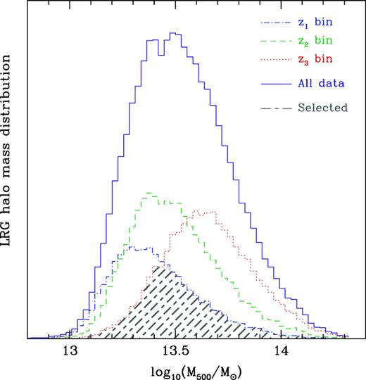
The halo mass distributions of the LRG samples in different redshift ranges. The blue, green, and red dashed curves are for z1, z2, and z3 bins, respectively. The mass distribution of the whole redshift range is denoted in solid purple curve. The grey hatched region shows the selected sub-samples, which are used in our analysis, with the same mass distribution for the three z-bins.
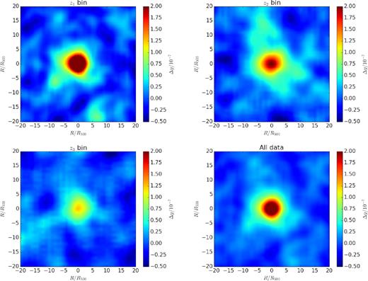
Fig. 2 shows the average y-map stacked against 11 660 LRGs at z1, z2, and z3 bin, respectively, with the same mass distribution. The corresponding y-profiles as a function of angular scale θ with their 1σ statistical uncertainties are shown in Fig. 3. The uncertainties are estimated by a bootstrap resampling by drawing a random sample of LRGs in a redshift bin. For example, in z1 bin, 11 660 LRGs are resampled from the total of 18 083 LRGs with a replacement allowed. For the mass distribution to be unchanged, we replace an LRG with another LRG of the same mass. We repeat this process 1000 times and the bootstrapped data produce 1000 average y-profiles. The rms fluctuation of the profiles is shown as an uncertainty in Fig. 3. We find that the average y-profiles have central peaks of y = (3.3 ± 0.2) × 10−7 in z1 bin, y = (1.7 ± 0.2) × 10−7 in z2 bin, y = (1.3 ± 0.2) × 10−7 in z3 bin, and y = (2.1 ± 0.1) × 10−7 for all data summed over the three redshift bins. As can be seen, we detect the tSZ signal out to ∼30 arcmin that is well beyond the Planck beam of 10 arcmin. Note that there are correlations between different angular scales when deriving y-profiles. The correlation coefficient matrices in different redshift ranges are shown in Fig. 4. Therefore, instead of using the independent errors shown in Fig. 3, we adopt the full covariance matrix to estimate the χ2 in the fitting process.
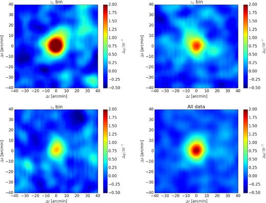
The stacked y-intensity maps for z1 bin (upper left), z2 bin (upper right), z3 bin (bottom left), and the whole redshift range with all LRG data (bottom right). The number of selected LRGs stacked in each map is 11 660 with the same mass distribution as shown in Fig. 1. The mean tSZ intensity in the annular region between 30 and 40 arcmin has been subtracted as the local background.
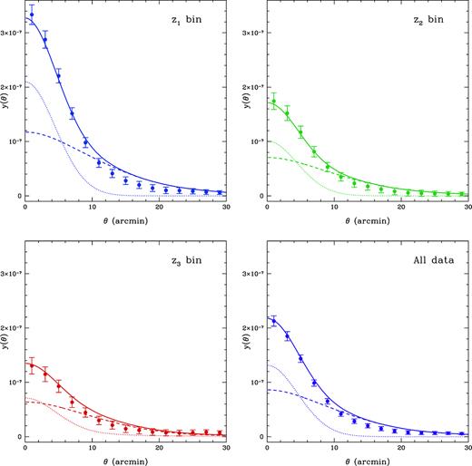
The angular cross-correlations of tSZ signal and galaxy cluster distribution in different redshift ranges. The data points are derived from the stacked intensity maps shown in Fig. 2. The error bars are simply derived from the diagonal elements of the covariance matrix in each case. The solid, dotted, and dashed curves are the best fits of total, one-halo, and two-halo correlation functions, respectively. All of data points and curves are rescaled based on the average values of corresponding intensities between 30 and 40 arcmin.
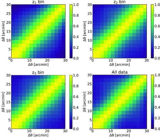
The correlation coefficient matrices between angular scales for the y-profiles y(θ) in different redshift ranges. The angular scale θ has been divided into 15 bins with Δθ = 2 arcmin.
We also notice that, given the same angular scale θ, y(θ) actually cover different physical scales of clusters at different redshifts. To investigate the stacked tSZ signal at the same cluster physical scales, and as a comparison, we also derive the stacked y-profiles as a function of r/R500, where r is the physical scale of radius. The corresponding y(r/R500) results are shown in the Appendix. In principle, the results of constraints on the UPP parameters do not depend on whether physical or angular scale is chosen, as long as the same theoretical halo model is used to compare with the same data sets. Since it has great convenience for the y(θ) when convolving with the beam function (as shown in Sec. 3.2), and considering accuracy and time consumption in the computation process, we choose to use y(θ) in our following discussion.
3 STACKED tSZ PROFILE MODELLING
3.1 Compton y-parameter
3.2 Theoretical stacked tSZ profile
3.3 Predicted stacked tSZ profile
3.3.1 Separating into mass and redshift bins
Using such a binning strategy, the computation speed becomes faster since we do not need to calculate the |$\mathcal {O}(10^{4})$| number of y(θ) profile individually. To verify the accuracy of such approach, we compute the |$\bar{y}(\theta)$| for such binning strategy and the individual sum up, and the difference is only at ∼1 per cent at most in different redshift ranges. Hence, we will use this scheme to compute the one-halo term as follows (see equation 19).
3.3.2 One-halo term
Since we have the information of LRG redshift z, M500, and R500, we can directly predict the one-halo term for each cluster, instead of using the halo mass function dn/dM in equation (11).
3.3.3 Two-halo term
4 FITTING METHOD
We employ the Markov Chain Monte Carlo (MCMC) method to perform constraints on the free parameters in the UPP. The Metropolis-Hastings algorithm is adopted to determine the accepting probability of the new chain points (Metropolis et al. 1953; Hastings 1970). The proposal density matrix is obtained by a Gaussian sampler with adaptive step size (Doran & Muller 2004). We assume uniform flat priors for all the free parameters, and their ranges are set to be P0 ∈ (0, 20), c500 ∈ (0, 10), α ∈ (0, 10), and β ∈ (0, 10). We also add a free parameter η on the power-law index of E(z) in equation (6), when simultaneously fitting the three redshift bins together. This parameter can adjust the redshift-dependence of the electron pressure profile, and we set η ∈ (−10, 10). We run fifteen parallel chains for each case we explore, and obtain 105 chain points for one chain after it reaches the convergence criterion (Gelman & Rubin 1992). After performing the burn-in and thinning the chains, we merge all chains together and obtain about 10 000 chain points to illustrate one-dimensional (1D) and 2D PDFs of the free parameters.
5 RESULTS OF CONSTRAINTS
In Fig. 3, we show the fitting results for different redshift ranges. The solid, dotted, and dashed curves are the best fits of total, one-halo, and two-halo correlation functions, respectively. Note that we use the covariance matrix between different angular scales instead of the error bars shown in Fig. 3 in the fitting process. These error bars are simply derived from the diagonal elements of the corresponding covariance matrix. As shown in Table 1, We find that the minimum reduced chi-square, which is defined by |$\chi ^2_{\rm red}=\chi _{\rm min}^2/(N-M)$|, where N and M are the number of data and free parameters in the model for the three main redshift bins and the whole range with all LRG data are 1.65, 0.45, 0.52, and 1.88, respectively. This indicates that the data can be well fitted in each case, expecially for the z2 and z3 bins.
| Case | P0 | c500 | α | β | γ | η | |$\rm \chi ^2_{\rm red}$| |
|---|---|---|---|---|---|---|---|
| z1 bin | |$3.35^{+8.18}_{-1.35}$| | |$1.45^{+0.56}_{-0.41}$| | |$4.31^{+0.66}_{-2.88}$| | |$5.14^{+3.00}_{-0.86}$| | 0.31 | – | 1.65 |
| z2 bin | |$10.46^{+1.54}_{-6.85}$| | |$1.88^{+0.53}_{-0.55}$| | |$4.03^{+0.96}_{-2.79}$| | |$4.39^{+3.45}_{-0.79}$| | 0.31 | – | 0.45 |
| z3 bin | |$6.15^{+5.25}_{-3.67}$| | |$2.23^{+2.42}_{-0.80}$| | |$1.24^{+3.68}_{-0.50}$| | |$3.00^{+0.43}_{-0.30}$| | 0.31 | – | 0.52 |
| All data | |$2.18^{+9.02}_{-1.98}$| | |$1.05^{+1.27}_{-0.47}$| | |$1.52^{+1.47}_{-0.58}$| | |$3.91^{+0.87}_{-0.44}$| | 0.31 | – | 1.88 |
| 3 bins | |$3.04^{+15.53}_{-1.93}$| | |$2.12^{+0.82}_{-1.01}$| | |$5.80^{+3.89}_{-4.46}$| | |$4.83^{+2.20}_{-0.78}$| | 0.31 | – | 1.61 |
| 3 bins with η | |$2.99^{+3.44}_{-1.57}$| | |$1.16^{+0.79}_{-0.29}$| | |$2.66^{+1.67}_{-0.97}$| | |$5.48^{+2.39}_{-1.38}$| | 0.31 | |$-3.11^{+1.09}_{-1.13}$| | 1.39 |
| A10 | 8.403 |$h_{70}^{-3/2}$| | 1.177 | 1.0510 | 5.4905 | 0.3081 | – | – |
| Planck13 | 6.41 | 1.81 | 1.33 | 4.13 | 0.31 | – | – |
The corresponding best fits and 1σ errors of P0, c500, α, and β are shown in Table 1, and the 1D PDFs are given in Fig. 5. We find that the P0 is not well constrained by the data, and its 1D PDFs extend in large parameter space with a wide peak between 2 and 11 in different redshift ranges. The constraint result of c500 in each case is in a good agreement that the probability peaks are around 1.5, although the width of the PDF of the z3 bin is wider than others. We do not obtain stringent constraints on α in the three z-bins separately. As can be seen, the PDFs have flat tops extending from 1.5 to 4.5 for the z1, z2, and z3 bins. The constraint is significantly improved for the all-data case with a peak at 1.5. For β, we find that the results of the z2 and z3 bins are well consistent, while the best-fitting value is apparently smaller in the z3 bin.
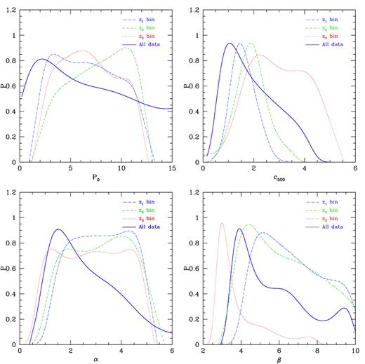
The 1D PDFs of P0, c500, α, and β in different redshift ranges. The blue dash–dotted, green dashed, and red dotted curves are the results in z1, z2, and z3 bins, respectively. The solid purple curve is for the whole redshift range with all stacked data.
We also find that, generally, the fitting results of the four cases are consistent with that given by Arnaud et al. (2010) and Planck Collaboration V (2013), especially for the all-data case (e.g. the constraints on c500, α, and β). This implies that our method is feasible and effective for the studies of the cluster electron pressure profile. Beside, as indicated in Table 1, there is noticeable evolution of the parameters, i.e. c500, α, and β, in the three redshift bins. We can see that α, and β become smaller and smaller as the redshift increases, while c500 tends to be larger at high redshift.
In order to suppress the fitting uncertainties of the free parameters and check the consistency of the UPP model in different redshift bins, we also try to simultaneously fit the data in the three redshift bins using |$\chi ^2_{\rm 3bins}=\chi ^2_{z_1}+\chi ^2_{z_2}+\chi ^2_{z_3}$|. As shown in the left-hand panel of Fig. 6, we find that the data can be fitted with |$\chi ^2_{\rm red}=1.61$| (see Table 1), adopting the usual model of electron UPP with four free parameters, i.e. P0, c500, α, and β.4 However, we can see that, except for the z2 bin, the theoretical curves cannot fit the data very well within angular scales less than 5 arcmin in the z1 and z3 bins.
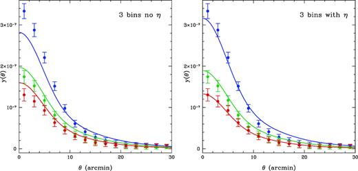
Left: The fitting result of ycross(θ) by simultaneously fitting the three redshift bins without parameter η. Right: The same as left-hand panel but η included. As can be seen, the data cannot be well fitted within θ < 5 arcmin in the z1 and z3 bins in the left-hand panel, and it can be improved by including η as shown in the right-hand panel.
Since we can find that, by comparing to the data, the predicated curve is lower in the z1 bin, and higher in the z3 bin, we can adjust the redshift dependence of the model by adding a free parameter η on the power-law index of E(z) in equation (6) (i.e. E(z)8/3 → E(z)8/3 + η). In the right-hand panel of Fig. 6, we show the fitting result when including η. We can find that the fitting results are significantly improved with |$\chi ^2_{\rm red}=1.39$|, that is ∼5 smaller for the |$\chi ^2_{\rm min}$| than the case without η (see Table 1). We find that the best fit of η is |$-3.11^{+1.09}_{-1.13}$|, which significantly changes the previous power-law index (i.e. 8/3) of E(z). This indicates that our result prefers weaker redshift dependence for the cluster gas pressure model.
The 1D PDFs and 2D contour maps of the free parameters for the three bins with and without η are shown in Fig. 7. The 1σ (68.3 per cent), 2σ (95.5 per cent), and 3σ (99.7 per cent) confidence levels are shown here. We can find that the fitting results of the three bins with and without η are basically consistent with each other. Besides, by comparing to fig. 5 in Planck Collaboration V (2013), we find that our constraint results (contours and 1D PDFs) are in a good agreement with their results, and our method can even offer more stringent constraints on c500 and β. The constraint can be further improved in the future with more LRG sample included.
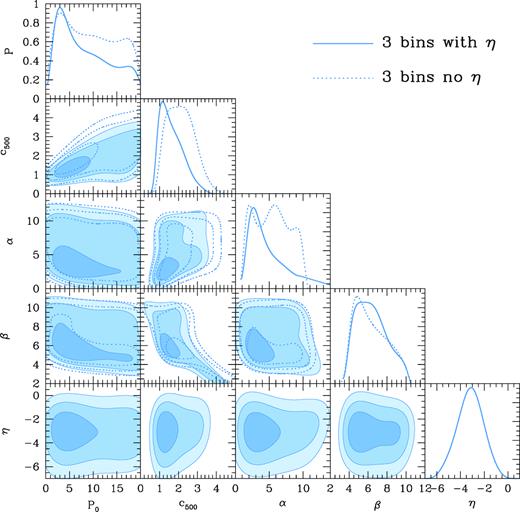
The contour maps and 1D PDF of free parameters when fitting the data of all three bins with and without η. The 68.3 per cent, 95.5 per cent, and 99.7 per cent confidence levels are shown. We can find that the best fit of |$\eta =-3.11^{+1.09}_{-1.13}$|, which significantly changes the power-law index 8/3 of E(z) in equation (6). This indicates that our result prefers weaker redshift dependence of the electron pressure profile than Arnaud et al. (2010).
6 SUMMARY AND DISCUSSION
In this work, we make use of the cross-correlation between the tSZ signal measured by Planck satellite and LRGs from SDSS DR7 to study the UPP of galaxy clusters. We first stack the Planck y-map against the LRGs and derive the mean y-profile. The LRG sample is given by SDSS DR7 with 0.16 < z < 0.47 and 3 × 10¹² ≲ M500 ≲ 3 × 10¹⁴|$\rm {{\rm M}_{\odot }}$|. In order to study the redshift evolution of the properties of intra-cluster gas, we divide the LRG sample into sub-samples in three redshift bins. We find that the peaks of the mass distributions in the three redshift bins move towards higher halo mass as the redshift increases. In order to remove the effect of non-matching mass distribution in our analysis, we select sub-sample from each redshift bin with the same mass distribution.
Then we derive theoretical stacked tSZ y-profile with the help of the halo model. The Planck beam function is also considered in the estimates. To obtain more realistic and accurate predictions, we take into account of the information from measurements, such as the redshift, M500, and R500, and simplify the calculation by dividing the LRG sample into sub-redshift and mass bins. We adopt the MCMC technique to illustrate the probability distribution of the parameters in the gas pressure profile, and set wide parameter ranges as prior distributions.
We separately fit the y-profile data obtained from the stacked y-map in the z1, z2, and z3 redshift bins, and the whole redshift range with all stacking data. We find that the fitting results of the four parameters, i.e. P0, c500, α, and β, are mainly consistent with one another. They are also in a good agreement with the results from Arnaud et al. (2010) and Planck Collaboration V (2013), especially for the all-data case. We find that there is evolution for c500, α, and β from the low to high redshift that the best fits of α, and β become smaller, while c500 becomes greater as the redshift increases.
In order to further investigate the redshift evolution and check the consistence of the UPP model at different redshift bins, we fit the data in the three redshift bins simultaneously by summing up the χ2 of the three bins together. Interestingly, we find that the UPP model cannot provide good fits on the data at θ < 5 arcmin in the z1 and z3 bins. After checking the results, we propose to add a parameter η on the power-law index of E(z) to change the redshift dependence of the model. The best-fitting value of η is |$-3.11^{+1.09}_{-1.13}$|, which suggests that the power index of redshift evolution of the UPP profile should be equal to |$\eta +8/3=-0.44^{+1.09}_{-1.13}$|. This result implies that the UPP profile may be less redshift dependent than its original form. Physically, this result indicates that the cluster pressure profile is less evolved than it was thought to be, and Compton y-profile could be nearly redshift independent. By including this factor, we find the |$\chi ^2_{\rm red}$| decreases from 1.61 to 1.39, which is ∼5 smaller in |$\chi ^2_{\rm min}$| than that given by the usual UPP model. By comparing the 1D and 2D PDFs with Planck Collaboration V (2013), we find our results from the three bins with and without η cases can match theirs very well, and can even offer more stringent constraints on c500 and β. This indicates that our method can provide reliable results that prefer less redshift dependence of the UPP mode. We will include more samples and further confirm our result in the future work, e.g. analysing the SDSS DR12 data, and provide more accurate constraints on the cluster pressure profile.
Besides, this study also can be an important step towards fully quantify the distribution of missing baryons. This is because, a significant amount of baryons are associated with filaments, voids and sheets which have much weaker signals of SZ effect than haloes (Haider et al. 2016). As one can see in Tanimura et al. (2019a), the stacked SZ signal of the filaments is usually entangled with the halo contribution. Therefore, improvement on the halo model’s pressure profile will lead to a more precise subtraction of the halo contribution, and will result in better measurement of the signals from filaments and sheets. Although this is out of the scope of this paper, our study can eventually contribute to the more precise determination of the baryons within filaments and sheets.
ACKNOWLEDGEMENTS
YG acknowledges the support of NSFC-11822305, NSFC-11773031, NSFC-11633004, the Chinese Academy of Sciences (CAS) Strategic Priority Research Program XDA15020200, the NSFC-ISF joint research programme no. 11761141012, and CAS Interdisciplinary Innovation Team. YZM is supported by the National Research Foundation of South Africa with grant no. 105925, no. 110984, and NSFC-11828301. This research has been also supported by funds from the European Research Council (ERC) under the Horizon 2020 research and innovation programme grant agreement of the European Union: ERC-2015-AdG 695561 (ByoPiC, https://byopic.eu).
Footnotes
We also check the fitting result by setting γ as a free parameter, and the result is almost the same (but with wider PDFs).
REFERENCES
APPENDIX: STACKED tSZ PROFILE IN PHYSICAL SCALES
In order to stack the tSZ signal at the same physical scales from each LRG, we stack the Planck y-map at the positions of LRGs in physical coordinates, instead of angular coordinate. We reset a 2D physical coordinate system of −20 < r/R500 < 20 and −20 < r/R500 < 20, divided in 80 × 80 bins. The local background region is also redefined in physical scale, which is an annular region between |r/R500| = 15 and 20 for each LRG. Then, we follow the same procedure as described in Section 2.3 for stacking. After removing the LRGs with |$\ge 20{{\ \rm per\ cent}}$| masked region within a r/R500 = 20 circle, we obtain 18 117, 29 074, and 26 401 LRGs, respectively, for the z1, z2, z3 bins, and total 73 592 in the whole redshift range. We finally select 11 926 LRGs in each redshift bin with the same mass distribution. This mass distribution is quite similar with that in the y(θ) case.
The y-maps, cross-correlations of tSZ signal and galaxy cluster distribution, and correlation coefficient matrices between physical scales in the y(r/R500) case are shown in Figs A1–A3, respectively. By comparing to the y(θ) case, as shown in Figs 3 and A2, we find that there is a bump feature around r/R500 ∼ 10 in the y(r/R500) profiles, especially for the z1 bin, which is mainly due to the two-halo term. This feature is smoothed out in the y(θ), since it is obtained by stacking different cluster physical scales at the same angular scale θ.
The stacked y-intensity maps for z1 bin (upper left), z2 bin (upper right), z3 bin (bottom left), and the whole redshift range with all LRG data (bottom right). The number of selected LRGs stacked in each map is 11 926 with the same mass distribution. The mean tSZ intensity in the annular region between r/R500 = 15 and 20 has been subtracted as the local background.
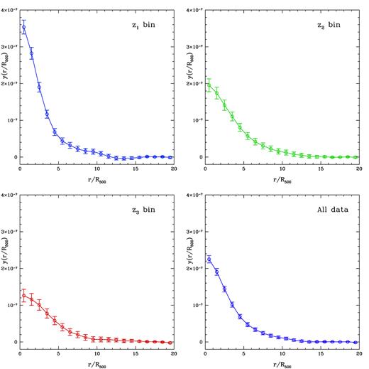
The cross-correlations of tSZ signal and galaxy cluster distribution as a function of r/R500 in different redshift ranges. The error bars are simply derived from the diagonal elements of the covariance matrix in each case. All of data points are rescaled based on the average values of corresponding intensities between r/R500 = 15 and 20.
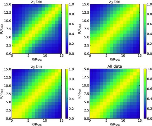
The correlation coefficient matrices between physical scales for the y-profiles y(r/R500) in different redshift ranges. The scale r/R500 has been divided into 15 bins.
