


ABSTRACT
To better understand the origin and evolution of the Milky Way bulge, we have conducted a survey of bulge red giant branch and clump stars using the High Efficiency and Resolution Multi-Element Spectrograph on the Anglo–Australian Telescope. We targeted ARGOS survey stars with predetermined bulge memberships, covering the full metallicity distribution function. The spectra have signal-to-noise ratios comparable to, and were analysed using the same methods as the GALAH survey. In this work, we present the survey design, stellar parameters, distribution of metallicity, and alpha-element abundances along the minor bulge axis at latitudes b = −10°, − 7.5°, and −5°. Our analysis of ARGOS stars indicates that the centroids of ARGOS metallicity components should be located ≈0.09 dex closer together. The vertical distribution of α-element abundances is consistent with the varying contributions of the different metallicity components. Closer to the plane, alpha abundance ratios are lower as the metal-rich population dominates. At higher latitudes, the alpha abundance ratios increase as the number of metal-poor stars increases. However, we find that the trend of alpha-enrichment with respect to metallicity is independent of latitude. Comparison of our results with those of GALAH DR2 revealed that for [Fe/H] ≈ −0.8, the bulge shares the same abundance trend as the high-α disc population. However, the metal-poor bulge population ([Fe/H] ≲ −0.8) show enhanced alpha abundance ratios compared to the disc/halo. These observations point to fairly rapid chemical evolution in the bulge, and that the metal-poor bulge population does not share the same similarity with the disc as the more metal-rich populations.
1 INTRODUCTION
Despite its prominent role in the formation and evolution of the Galaxy, the bulge is perhaps the least understood stellar population. The bulge is host to a great diversity of stars, with up to five peaks in its metallicity distribution function (MDF; Ness et al. 2013a; Bensby et al. 2017), including some of the oldest stars in the Galaxy (see e.g. Howes et al. 2015; Nataf 2016; Barbuy, Chiappini & Gerhard 2018; for a review). It is also a major Galactic component, comprising 30 per cent of the Milky Way’s total mass (Portail et al. 2015; Bland-Hawthorn & Gerhard 2016). Studies of the bulge are therefore essential for understanding the formation and evolution of the Milky Way, and by inference, other spiral galaxies.
Galaxy bulges are typically referred to either as a ‘classical’ or ‘pseudo’-bulge (Kormendy & Kennicutt 2004). Classical bulges are thought to have formed via rapid dissipative collapse consistent with λCDM cosmological predictions (White & Rees 1978; Rahimi et al. 2010; Tumlinson 2010). The properties of classical bulges largely mirror that of elliptical galaxies: they consist of old stars with random stellar motions. On the other hand, pseudo-bulges, formed via secular evolution are flatter in shape, contain younger stars, and show evidence of cylindrical rotation (Kormendy & Kennicutt 2004). While most nearby galaxies appear to have a pseudo-bulge, some contain both types of bulges (Fisher & Drory 2011; Erwin et al. 2015). The traditional view of the Galactic bulge is that it is exclusively old (>10 Gyr), based on the observed colour–magnitude diagram in multiple fields (e.g. Zoccali et al. 2003; Clarkson et al. 2008). Using Hubble Space Telescope photometry, Clarkson et al. (2011) and Bernard et al. (2018) estimated the young stellar population (<5 Gyr) in the bulge to be <3.4 per cent and 11 per cent, respectively.1 Early detailed abundance studies of the bulge corroborated this view: bulge giants are typically overabundant in α-elements such as O, Si, and Ti, but especially so in Mg (e.g. McWilliam & Rich 1994; Zoccali et al. 2006; Lecureur et al. 2007). Fulbright, McWilliam & Rich (2007) suggested that the abundances of bulge stars plateau at [Mg/Fe] = 0.3 dex even at supersolar metallicity, and the bulge has a separate chemical enrichment to the disc in the solar neighbourhood. Furthermore, multiple authors found a vertical metallicity gradient in the bulge (Minniti et al. 1995; Zoccali et al. 2008). Together these results were interpreted as signatures of a classical bulge population, formed early and rapidly via mergers or dissipational collapse prior to the formation of the disc (e.g. Matteucci & Brocato 1990).
The discovery of a significant fraction of young (<5 Gyr), relatively metal-rich ([Fe/H] > −0.4) microlensed bulge turn-off and subgiant stars thus came as a surprise (Bensby et al. 2013, 2017).2 The presence of such stars would be inconsistent with the classical scenario and instead point to disc-instabilities channelling stars from the disc into the bulge (e.g. Athanassoula 2005; Martinez-Valpuesta & Gerhard 2013; Di Matteo et al. 2014; Fragkoudi et al. 2018). Abundance studies now suggest that the Milky Way bulge and thick disc share strong chemical similarities. Meléndez et al. (2008) found that the α-abundance trends in the bulge follow that of the local thick disc. Alves-Brito et al. (2010) reached the same conclusion from their re-analysis of Fulbright et al. (2007); as have many recent studies (Gonzalez et al. 2011; Johnson et al. 2014; Ryde et al. 2016; Bensby et al. 2017). However, Bensby et al. (2017) observed that their microlensed bulge stars lie in the upper envelope of the thick disc, implying that the bulge may have experienced a faster chemical enrichment than typical thick disc stars in the solar neighbourhood. An increasing number of kinematic studies show that the bulge rotates cylindrically (Kunder et al. 2012; Ness et al. 2013b; Zoccali et al. 2014; Molaeinezhad et al. 2016; Ness et al. 2016), which is also evidence against a primarily classical bulge population. Furthermore, infrared imaging reveal that the bulge is ‘boxy’, or X-shaped (Dwek et al. 1995; Ness & Lang 2016), and the split red clump observed in photometric studies is often attributed to this X-structure (McWilliam & Zoccali 2010; Wegg & Gerhard 2013; Nataf et al. 2015; Gonzalez et al. 2015b; Zasowski et al. 2016; Ciambur, Graham & Bland-Hawthorn 2017).3 The most recent observational evidence thus point to a primarily pseudo-bulge population in the Milky Way.
The MDF of the bulge has proven to be complex that there is not yet a consensus on the metallicity range (see Barbuy et al. 2018 for a review). Many studies have shown that it is composed of multiple components (e.g. Babusiaux et al. 2010; Hill et al. 2011; Ness et al. 2013a; Zoccali et al. 2014; Rojas-Arriagada et al. 2017; García Pérez et al. 2018). In particular, Ness et al. (2013a) showed that there are up to five components based on ≈14 000 bulge red-giant stars. They associated stars with [Fe/H] ≈ −0.5 with the inner thick disc, while the more metal-rich populations with mean [Fe/H] = −0.2 and +0.2 differ in their kinematics such that stars with the highest metallicity are more prominent near the plane. Ness et al. (2013a) concluded that these metal-rich populations originated in different parts of the early thin disc due to bar-induced disc instabilities. The strength of each MDF component varies with latitude, manifesting as the vertical metallicity gradient seen in earlier studies. Thus, the vertical metallicity gradient cannot be interpreted as a signature of merger or dissipative collapse bulge formation (Zoccali et al. 2008; Babusiaux et al. 2010; Ness et al. 2013a; Rojas-Arriagada et al. 2017). In agreement with Ness et al. (2013a), Bensby et al. (2017) found five peaks in their MDF for a much smaller sample of microlensed bulge dwarfs and subgiants, four of which matched the ARGOS MDF peaks. The sample age distribution of microlensed bulge stars also show multiple peaks that could be interpreted as star formation episodes in the bulge. Bensby et al. (2017) suggested that the peaks at 11 and 8 Gyr could be the onset of the thick and thin discs; and at 6 and 3 Gyr could be associated with the younger parts of the thin disc/Galactic bar.
It is possible that a classical bulge component exists in the Milky Way despite mounting evidence for a predominantly pseudo-bulge population. Studies have shown that fields at latitudes |b| > 5 have a combination of X-shaped and classical bulge orbits (Ness et al. 2012; Uttenthaler et al. 2012; Pietrukowicz et al. 2015). In addition, the most metal-poor bulge RR Lyrae stars do not show characteristics of the boxy bulge, such as cylindrical rotation (Dékány et al. 2013; Kunder et al. 2016). Spatial and kinematic results from the GIBS survey (Zoccali et al. 2017) indicate that the metal-poor population of the bulge is centrally concentrated and rotates more slowly than the metal-rich population, although the authors do not argue strongly for a classical component. If such a component did exist, disentangling it from those originated in the disc may be very challenging (Saha 2015). Schiavon et al. (2017) have shown that chemical abundances can serve as a powerful diagnostic for identifying subpopulations in the bulge, having found possible evidence of a dissolved globular clusters using APOGEE abundances.
Studies of the bulge have previously been hindered by high extinction in the bulge region, and the faintness of bulge stars. The sample sizes are typically small if observed at high resolving power (e.g. Johnson et al. 2014; Bensby et al. 2017; Jönsson et al. 2017). While alpha abundance trends are well established for bulge stars with results from the GIBS, Gaia–ESO, and APOGEE surveys (Gonzalez et al. 2015a; Rojas-Arriagada et al. 2017; Schultheis et al. 2017), information on other elements, especially the neutron-capture elements, are still scarce (Johnson et al. 2012; Van der Swaelmen et al. 2016). In this paper, we present the High Efficiency and Resolution Multi-Element Spectrograph (HERMES) Bulge Survey (HERBS), which was designed to be in synergy with the GALAH survey (De Silva et al. 2015). Here, we aim to provide a large chemical inventory for stars in the bulge by leveraging the wavelength coverage of the HERMES spectrograph, which allows us to obtain chemical abundances for up to 28 elements, including the light, alpha, iron-peak, and heavy elements. In addition, we will be using similar spectroscopic analysis method and linelist to the GALAH survey, which facilitates a consistent comparison of the chemical properties of bulge and disc stars.
2 DATA DESCRIPTION
2.1 Target selection
For our observations, we selected giants and red clump stars from the analysed sample of the ARGOS survey (Freeman et al. 2013; Ness et al. 2013a). ARGOS stars were selected to be between magnitude K = 11.5–14 from the 2MASS catalogue (Skrutskie et al. 2006), with J, K magnitude errors <0.06 and all quality flags = 0 (Freeman et al. 2013). To exclude most dwarfs, a colour cut in (J − K)0 = 0.38 was made; each of the ARGOS field was de-reddened using the Schlegel, Finkbeiner & Davis (1998) reddening map. The magnitude and colour selection of ARGOS aimed to minimize very cool and metal-rich giants, but at the same time include very metal-poor giants (Freeman et al. 2013). Any remaining foreground dwarfs are excluded after the ARGOS stellar parameters analysis based on their surface gravity.
In order to exclude background and foreground giants, distances were used to infer |RGC| for each star. Ness et al. (2013a) computed stellar distances by assuming that stars between log (g) = 1.8–3.2 and Teff = 4500–5300 K are clump giants, and have absolute magnitude MK = −1.61 ± 0.22 (Alves 2000). For stars that are not located near the clump, MK is obtained by matching stellar parameters with the closest point on a grid of 10 Gyr BaSTI isochrones. The error of red clump based distances is ≈15 per cent, and ≈38 per cent for isochrone-based distances. Ness et al. (2013a) noted that their red clump sample could be contaminated with non-clump giants, but this contamination should be small. Furthermore, a small subset of their sample shows that isochrone only and red clump only distances return consistent results (Ness et al. 2013a). The ARGOS study defined the bulge region to be within Galactocentric radius |RGC| ≤ 3.5 kpc.
This study aims to obtain a thorough chemical inventory of red clump and giant stars, probing the different subpopulations found by Ness et al. (2013a) and their variation with latitude. We have therefore used the ARGOS RGC and [Fe/H] measurements to select stars that most likely reside in the bulge region, i.e. those with |RGC| ≤ 3.5 kpc, and gave greater weights to more metal-poor/metal-rich stars in the selection process. We achieved this by allocating ≈100 per cent of ARGOS stars at low and high metallicity, and ≈50 per cent elsewhere. This ensures that we cover the entire metallicity range and all subpopulations in each field, especially increasing the relative fraction of metal-poor stars.
Because the integration time required for faint bulge stars is much greater for HERMES than AAOmega (see the next section for details), we could only observe a few ARGOS fields to complete the project in a feasible time frame. Fig. 1 shows locations of the observed fields (the shaded blue), which includes three ARGOS fields along the minor axis at (ℓ, b) = (0, 5); (ℓ, b) = (0, −7.5); (ℓ, b) = (0, −10). In addition to the ARGOS fields, we observed the field (ℓ, b) = (2, −3), which was selected due to its relative low extinction and it being covered by K2, which could in principle provide accurate age estimates from asteroseismology (e.g. Silva Aguirre et al. 2015). We also added suitable bulge metal-poor candidates ([Fe/H]EMBLA < −1.5) from the EMBLA survey (Howes et al. 2016) to fields (0,−10) and (0,−5).
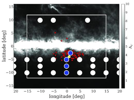
Locations of bulge fields observed by the HERBS survey, shown in the blue circles. Also shown are ARGOS fields (the white circles, Ness et al. 2013a), microlensed stars (the red stars, Bensby et al. 2017), and Baade’s Window (the yellow circle). The white square indicates roughly the bulge vicinity, and the background map shows the dust extinction.
2.2 Observations
The observations were taken using the HERMES spectrograph (Sheinis et al. 2015) on the 2dF system of the Anglo–Australian Telescope. The pilot survey, which targeted field (0, −7.5) was completed in 2014 August, and observations of the remaining fields were completed between 2015 May and 2016 June.
The 2dF system contains two observing plates that cover a 2° diameter field of view. Each 2dF plate has a set of 400 optical fibres, each of them 2 arcsec in diameter. Of these, eight fibres are dedicated to bright guide stars to maintain field position accuracy, 25 fibres are allocated to measuring sky variation across the field and typically ≈350–360 science objects were observed per field. Sky locations were chosen by visually inspecting DSS images of each field for blank regions. The instrument, HERMES, enables spectra of four wavelength intervals to be observed simultaneously: 4713–4903 Å (blue CCD); 5648–5873 Å (green CCD); 6478–6737 Å (red CCD), and 7585–7887 Å (IR CCD). The wavelength coverage of HERMES has been optimized for accurate stellar parameters and abundance measurements, including Balmer lines in the blue and red CCDs. At the nominal resolution of |$\lambda /\Delta \lambda \approx 28\, 000$|, HERMES can deliver abundances for up to 28 elements, including Li, O, Na, Mg, Al, Si, K, Ca, Sc, Ti, V, Cr, Mn, Co, Ni, Cu, Zn, Rb, Sr, Y, Zr, Ru, Ba, La, Sm, Ce, Nd, and Eu. Combined with the high multiplexity of 2dF/AAT, HERMES is a powerful tool for detail abundance studies of Galactic stellar populations.
While the optical wavelength coverage of HERMES provides a large number of abundances and accurate parameters, it is also a draw back for bulge observations. Due to the faintness of bulge stars and high extinction in this region, we require significantly longer integration times compared to, for example, ARGOS and APOGEE to achieve the required signal-to-noise ratio (SNR) for precise parameters and abundances. As stated in the previous section, ARGOS stars have 2MASS K magnitude 11.5–14, or an approximate V magnitude of 15–17 in the field (ℓ, b) = (0, −7.5). In contrast, typical GALAH targets have V magnitude of 12–14. We aimed to have the same data quality as the GALAH survey, which attains median SNR ≈ 100 per resolution element, or ≈50 per pixel, for the green CCD (Martell et al. 2017). To determine the required integration time, we observed field (ℓ, b) = (0, −7.5) over three consecutive nights and determined the signal to noise of co-added spectra in real time. This field has an apparent red clump magnitude of V ≈ 16, and after 10 h of observing time we reached the desired signal to noise. We scaled this time to estimate the required observing time of all other fields based on their apparent red clump magnitudes.
The long integration times meant that we must re-configure each field throughout the night to maintain position accuracy. To do this efficiently, we allocated the same set of stars to both 2dF plates, and alternated between them. Observing intervals are split into 30 min exposures to minimize the effect of cosmic rays. Calibration frames (fibre flats and ThXe arc frames) were taken either immediately before or after each exposure. Most of the observations were carried out in dark time, some during grey time. Lastly, due to the faint signals of our targets, we chose to observe in the NORMAL CCD read-out mode, to minimize read noise while maintaining reasonable overhead time.
Due to the large fraction of time lost (because of poor weather) over the course of this project, we were not able to complete the observations of fields (0,−5) and (2,−3). The (0,−5) field is lacking some 10 h, and (2,−3) requires approximately 25 additional hours. For this reason, we do not include the (ℓ, b) = (2, −3) field in our analysis as the signal to noise of this field would be insufficient to derive accurate stellar parameters and abundances.
The integration time and median SNR in the blue, green, and red CCDs of the minor axis fields are given in Table 1. We were able to achieve similar signal to noise to the GALAH survey for the pilot field at (ℓ, b) = (0, −7.5) and (0, −10). The median SNR for field b = −5° is much lower because we were not able to complete the planned observations for this field.
The estimated V-magnitude and median signal-to-noise ratio of each bulge field, except the (2,−3) field, which was not used in subsequent analysis due to low SNR. The IR arm is not shown as it has similar SNR to the red arm. For HERMES, one resolution element is equivalent to approximately 4 pixel or ≈0.2 Å.
| Field | RC | Exp time | SNRB | SNRG | SNRR |
|---|---|---|---|---|---|
| (ℓ, b) | Vmag | (h) | (pixel−1) | (pixel−1) | (pixel−1) |
| (0, −5) | 17.4 | 17 | 20 | 34 | 46 |
| (0,−7.5) | 16.3 | 10 | 32 | 51 | 65 |
| (0, −10) | 16.0 | 08 | 30 | 40 | 53 |
| Field | RC | Exp time | SNRB | SNRG | SNRR |
|---|---|---|---|---|---|
| (ℓ, b) | Vmag | (h) | (pixel−1) | (pixel−1) | (pixel−1) |
| (0, −5) | 17.4 | 17 | 20 | 34 | 46 |
| (0,−7.5) | 16.3 | 10 | 32 | 51 | 65 |
| (0, −10) | 16.0 | 08 | 30 | 40 | 53 |
3 DATA REDUCTION
Each 30 min observing block returns a data frame consisting of ≈380 spectra (including sky fibres). The data frames were reduced using the standard 2dF reduction package 2dfdr v6.46.4 The software subtracts bias level using the overscan, performs flat-field corrections, calibrates the wavelength using ThXe arclines and subtracts sky. For sky subtraction, we used the throughput mode, in which we calibrated the fibre throughput using strong skylines in the IR arm of HERMES. The reduced frames were checked by eye for consistency and data quality. Frames with low SNR due to clouds, or very poor seeing (>2 arcsec) were excluded after the reduction stage.
To correct for the telluric absorption, we convolved the NOAO atlas (Hinkle et al. 2000) to HERMES spectral resolving power (|$\mathcal {R}$| = 28 000). The atlas is scaled to match the typical absorption level at Siding Spring, and shifted by the barycentric velocity of each star. The wavelength points corresponding to telluric lines have their errors increased by the inverse of the telluric absorption level. Spectral pixels affected by tellurics have much lower weights and therefore will not contribute significantly to the spectral synthesis analysis (Section 5). Thereafter, each object spectrum is corrected for their barycentric velocity, interpolated on to a common wavelength grid and combined using the same averaging method described above. Examples of reduced spectra can be found in Fig. 2.
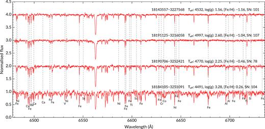
Example HERMES spectra in the ‘red’ wavelength region (which includes the H α line), normalized and shifted to rest using the guess code (Section 4). The stars’ 2MASS identification, SNR (per pixel), and sme-derived parameters are shown. Most of the lines used for stellar parameters and abundance analysis have been labelled.
We note that our data reduction process is independent of the GALAH reduction pipeline, most importantly we do not correct for the tilted point spread function (PSF) of HERMES spectra (Kos et al. 2017), which may reduce the resolution and signal to noise towards the corners of each CCD. The spectral resolving power is lowered by up to ≈15 per cent, and the SNR is lowered by up to ≈5 per cent (Kos et al. 2017). This affects all fibre bundles, but is minimized towards the CCD centre.
4 RADIAL VELOCITY AND INITIAL PARAMETER ESTIMATES
Having good estimates for the radial velocity and initial parameters significantly speed up the subsequent spectroscopic analysis. For this purpose, we use a modified version of the guess code,5 which is implemented in the GALAH survey for radial velocity measurements and has been shown to provide accurate initial parameters (see Kos et al. 2017).
Only the blue, green, and red HERMES CCDs are used in this step; the IR CCD is excluded as it does not have as many parameter-sensitive lines and is severely affected by telluric absorption. The guess code has two separate modules to compute radial velocity and stellar parameters. Radial velocities are calculated via cross-correlation with a grid of 15 AMBRE model spectra (de Laverny et al. 2012). The models have log g = 4.5, [Fe/H] = 0, and spans 4000–7500 K in Teff, at 250 K intervals. Prior to cross-correlation, a crude normalization is done by fitting a spline function over observed spectra, omitting regions around H α and H β lines. The normalized spectrum is then cross-correlated with all 15 models, one at a time. The cross-correlation peak is fitted with a quadratic function, the maximum of which is adopted as the cross-correlation coefficient. The coefficients range from 0 to 1, higher values indicate a better match between model and observation. To improve accuracy, model spectra that return coefficients less than 0.3 are excluded. The radial velocity is an average of values from accepted models, weighted by their cross-correlation coefficient. Each HERMES CCD goes through this process independently, and the final radial velocity is an average of all three CCDs, the uncertainty being the standard deviation between CCDs.
In general, our results show good agreement between the three CCDs, with the typical standard deviation being 0.4 km s−1. The radial velocity precision also compares well to that reported for the GALAH survey: 93 per cent of our sample have |$\sigma _{v_\mathrm{rad}} \le 0.6$| km s−1, whereas the typical GALAH radial velocity error is ≈0.5 km s−1 (Zwitter et al. 2018). Our precision may be affected by the lower SNR of the blue arm in particular, due to the high reddening level in the bulge region.
Estimates of stellar parameters (Teff, log g, [Fe/H]) were derived after the radial velocity determination using a grid of 16 783 AMBRE spectra. Spectra are shifted to rest with radial velocities from the previous step, and normalized by fitting third-order (for the blue and green arms) and fourth order (for the red arm) polynomials to predetermined continuum regions (by inspection of high-resolution spectra of the Sun, Arcturus, and μLeo). The polynomial orders are kept low to avoid poorly constrained continuum fits. From inspecting a large number of normalized spectra, the orders chosen appear to work best for the continuum variation of each CCD. Normalized spectra are interpolated on to the same wavelength grid as the models, and the L2 norm (distance in Euclidean space) between the observed and model spectra are computed. A linear combination of stellar parameters from 10 models that are closest in Euclidean space to the observed spectrum give the initial stellar parameters. These were used as starting models in the spectral synthesis analysis described in the next section.
5 SPECTROSCOPIC ANALYSIS
5.1 Stellar parameters
The stellar parameters and abundances pipeline and linelist we adopt is the same as that used in Data Release 2 of the GALAH survey (Buder et al. 2018). The atomic data are based on the Gaia–ESO survey linelist (Heiter et al. 2015a), consisting of mainly blend-free lines with reliable log (gf) values for stellar parameter determination. However, some background blending lines have slightly different gf values compared to the Gaia–ESO linelist, as they were changed to improve clearly discrepant fits to the HERMES Arcturus and Solar spectra.
For spectral synthesis, we used the code Spectroscopy Made Easy(sme) v360 (Valenti & Piskunov 1996; Piskunov & Valenti 2017). In this analysis, we implement the 1D, LTE marcs model atmospheres (Gustafsson et al. 2008). The atmospheric models uses spherical geometry with 1 M⊙ for log g ≤ 3.5, and plane-parallel otherwise. During the parameter-determination stage, we implement non-LTE corrections from Amarsi et al. (2016b) for Fe i lines.
Each spectrum is divided into several ≈10 Å wide segments containing lines relevant to stellar parameter determination. For this step, there are 20 segments containing line masks for Fe, Ti, and Sc. sme synthesizes the initial model based on the guess stellar parameters and radial velocity. In this first iteration, each segment is normalized using a linear function. sme then synthesizes lines of H α and H β; neutral and ionized lines of Sc, Ti, and Fe to determine Teff, log g, [M/H],6vsin i (rotational velocity), and vrad. The free sme parameter vrad is used to bring the model and data spectra to a common wavelength grid. The value of this parameter is typically in line with the radial velocity uncertainty. vrad is computed independently of other parameters and the same value is used to correct all segments.
The resolving power of HERMES is variable across the CCD image, in both the dispersion and aperture axes. A stable median value can be estimated by interpolating each segment with pre-computed resolution maps from Kos et al. (2017); this solution is implemented for the GALAH survey (Buder et al. 2018). However, since our spectra are combined from different fibres, we cannot recover the resolution information. Thus, in our sme analysis we adopted λ/Δλ = 28 000 throughout, and the variation in resolving power is incorporated as a component of vsin i. The synthetic spectra are convolved with a Gaussian instrumental broadening kernel.
Overall, our spectroscopic analysis returned fairly accurate stellar parameters for Gaia benchmark standards, and our reduction method provided similar results to the GALAH reduction pipeline (for details see Appendix A1). We found no significant offset in our effective temperature or surface gravity compared to reference values derived by Jofré et al. (2014) and Heiter et al. (2015b). The temperature offset is 40 K with standard deviation of 90 K; the surface gravity offset is 0.02 dex with standard deviation of 0.25 dex. The metallicity, however, shows an offset of −0.12 with standard deviation 0.08 dex. The metallicity offset is the same as that reported by the GALAH survey (Sharma et al. 2018). To remain consistent with GALAH, we have added +0.1 dex to all of our metallicity values. The standard deviation of the difference between our results and that of benchmark stars can be taken as typical uncertainties in the parameters Teff (90 K), log g (0.25 dex), and [Fe/H] (0.08 dex).
Fig. 3 shows the Kiel diagram for all minor axis fields. The stellar parameters are well represented by 10 Gyr isochrone tracks, which is what one expects for bulge giants. None of the ARGOS-selected stars turned out to be local dwarfs. Of the targets observed (≈350 per field), minus possible binaries and those with reduction issues, we have 313 stars analysed for field (0, −10), 13 of which are from the EMBLA survey. For the pilot field (0, −7.5), there are 315 stars in total. Part of the (0, −5) field was unfortunately affected by very strong hydrogen emission (at H α and H β rest wavelengths) from the interstellar medium. This affected the hydrogen line profiles for many stars, and as a result a large fraction of them failed to converge. Therefore, we only have 204 stars in field (0, −5) (two are EMBLA stars), giving us a grand total of 832 stars.
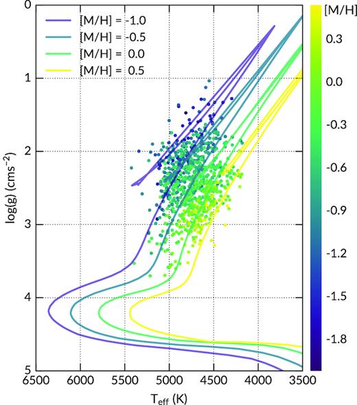
The Kiel diagram of the full sample (832 stars), overplotted with 10 Gyr parsec isochrones (Marigo et al. 2017) of metallicities indicated in the figure legend.
5.2 Elemental abundances
After the stellar parameters have been established, they are fixed for each abundance optimization. Similar to the parameters, sme optimizes the χ2 parameter to find the best-fitting abundance of each element. Only wavelength pixels within the line masks are used for χ2-minimization. During the optimization stage, sme de-selects blended wavelength points (if any) within the line masks. In this paper, we will report on abundances of the alpha elements O, Mg, Si, Ca, and Ti. For all elements except Ti, we computed the line-by-line abundances for each element and averaged the individual lines’ results, weighted by the abundance ratio uncertainties provided by sme. We do not include in the weighted average abundances that are flagged as upper limits. The Ti abundances are computed with the same lines also used for stellar parameters determination, and all lines were fitted at the same time. In addition, non-LTE corrections were applied to the elements O (Amarsi et al. 2016a), Mg (Osorio & Barklem 2016), and Si (Amarsi & Asplund 2017).
The alpha abundances presented here are not particularly sensitive to temperature, as shown in Fig. A2. We do not see any appreciable trends with Teff for the elements O, Si, and Ti. However, linear trends can be seen for Mg and Ca, which are also observed in GALAH data (Buder et al. 2018). While we note these issues, we do not apply empirical corrections to abundance-temperature trends, as the underlying physics is yet to be understood, and should be investigated further.
6 ARGOS COMPARISON AND METALLICITY DISTRIBUTION FUNCTIONS
As noted earlier, we selected most of our bulge stars from the ARGOS survey, which was observed with the AAOmega spectrograph (λ/Δλ =11 000). Figs 4 and 5 show the comparison between our parameters and that of ARGOS for stars in common. In Fig. 4, the differences are plotted as the histograms: the biases (median of the difference) are shown for Teff, log g, and [Fe/H]. The 1σ values in the figures were computed using the median absolute deviation (MAD) method, which is more robust to outliers. The standard deviations, after excluding 3σ outliers, are ΔTeff: 158 K, Δlog g: 0.38 dex, and Δ[Fe/H]: 0.16 dex. This comparison shows small offsets between the two studies. The standard deviation in Δ[Fe/H] is consistent with the combined HERBS and ARGOS metallicity uncertainties, and the overall bias is negligible. Even though ARGOS effective temperatures were determined using photometry (J − K0 colours), they agree remarkably well with our values and the standard deviation of ΔTeff is in line with the two studies’ combined uncertainty. Because the ARGOS photometric temperatures are less accurate at low latitudes due to increased extinction, field (0, −5) has a higher MAD value (143 K) compared to fields (0, −7.5) and (0, −10) (106 K and 111 K, respectively). Surface gravity shows a small 0.14 dex offset, but the standard deviation is expected of the combined HERBS and ARGOS log g uncertainties.

Histogram comparison between parameters derived in this work and those of ARGOS for stars in common. The differences are shown as (HERBS − ARGOS). The 1σ lines are median absolute deviations (MAD ≈ STD/1.4826 for Gaussian distributions).
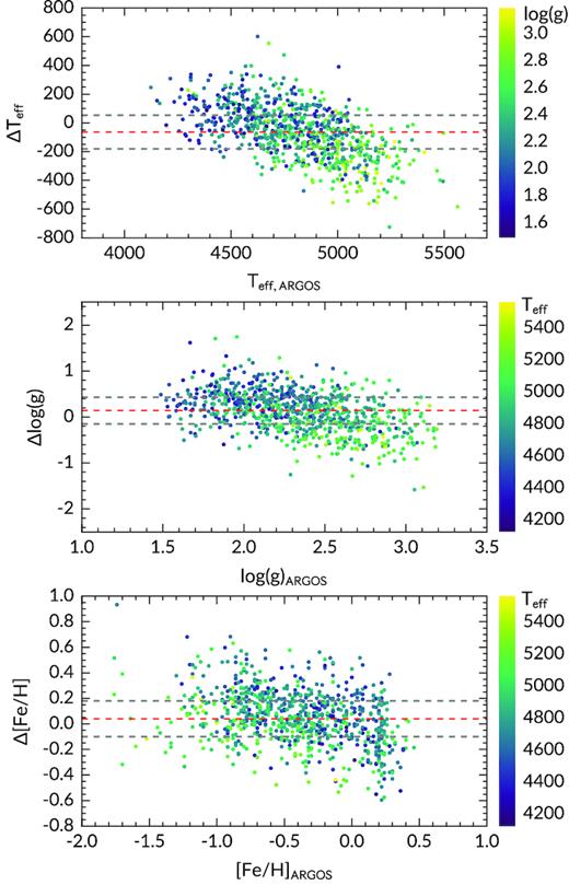
The same (HERBS − ARGOS) differences as Fig. 4, but plotted as a function of ARGOS stellar parameters, colour-coded by Teff or log g. Lighter colours represent warmer stars with higher surface gravities.
The metallicity distribution for each minor-axis field is shown in Fig. 6. Here, we have also overplotted the Gaussian distributions corresponding to each ARGOS component A–D: A being the most metal-rich; D the most metal-poor. As indicated above, our analysis suggests a slight compression of the ARGOS MDF. In Fig. 6, we have shifted the centroids of these components according to equation (6) to reflect this compression.
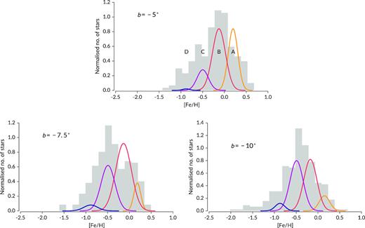
The metallicity distribution functions (the grey histograms) for the minor axis fields. Overplotted for comparison are ARGOS metallicity components A–D (corresponding to most metal-rich to most metal-poor). The ARGOS centroids have been shifted according to equation (6). The amplitude of each component has been multiplied by a factor of 2 to better match the distributions presented here, but their relative weights remain the same.
On the whole, our MDF appears flatter and wider compared to the ARGOS MDF, however, this is to be expected, as our selection function prioritized the most metal-rich and metal-poor stars. The selection criteria we employed have allowed for a larger fraction of metal-poor star to be observed. Approximately, 12 per cent of the stars have [Fe/H] ≤ −1, compared to the typical fraction of 4–5 per cent (Ness et al. 2013a; Rojas-Arriagada et al. 2017).
There are discussions in the literature regarding the number of metallicity components in the bulge, with some authors arguing for a two-component bulge metallicity distribution with much larger dispersions (Gonzalez et al. 2015a; Rojas-Arriagada et al. 2017; Schultheis et al. 2017), rather than three components with narrow dispersions (Ness et al. 2013a; García Pérez et al. 2018). As there are strong selection effects associated with our MDF, we are not able to directly address this issue. However, our analysis indicates that the ARGOS component centroids should be located ≈0.09 dex closer together. This difference is sufficiently small that for fields (0, −5) and (0, −10), the ARGOS components remain distinct given their narrow dispersions. However, for field (0, −7.5), the centroid of component A is within 1.5σ of component B’s centroid, meaning that there is a possibility components A and B are not distinct in field b = −7.5°. We re-analysed the ARGOS results for all three minor axis fields and found that fields (0, −5) and (0, −10) contain the same number of metallicity components as the original ARGOS decomposition. For field (0, −7.5), while component A becomes more difficult to distinguish, the revised MDF is not single peaked in the high-metallicity regime.
It is worth noting that the number of metallicity components may not be indicative of how many distinct populations reside in the Galactic bulge. Indeed, the N-body dynamical model of Fragkoudi et al. (2018) found that even though their bulge population originated from three different disc components, the final MDF is best described by two Gaussian curves with larger dispersions than the original disc components.
7 α-ELEMENT ABUNDANCES
The alpha elements are often associated with rapid SNe ii enrichment, and are thus useful indicators of formation/evolution time-scales for the different Galactic components (Tinsley 1979; Matteucci & Brocato 1990). Fig. 7 shows the alpha abundances from this study compared to recent high-resolution spectroscopic studies of bulge field stars in the literature. For this exercise, we have included Bensby et al. (2013, 2017), Johnson et al. (2014), and Gonzalez et al. (2015a). The Bensby et al. (2017) study includes all microlensed bulge dwarfs in Bensby et al. (2013), however, we use oxygen abundance ratios from Bensby et al. (2013), which is not available in the later study. The microlensed dwarfs were observed with the VLT/UVES spectrograph, KECK/HIRES spectrograph, or Magellan/MIKE spectrograph (|$\mathcal {R} \approx$| 40 000–90 000). Both Johnson et al. (2014) and Gonzalez et al. (2015a) provided individual abundances for a large number of bulge giants observed with the VLT/GIRAFFE spectrograph (|$\mathcal {R} \approx$| 22 500), but at different wavelength settings. All literature samples considered are smaller, but have on average higher SNR than our sample. Furthermore, only the oxygen abundance ratios from Bensby et al. (2013) were computed assuming non-LTE. All studies assumed LTE in their abundance analysis. On the whole, the scatter in HERBS abundance ratios is larger than the comparison samples and what could be expected from abundance ratio uncertainties from χ2-square fitting. This indicates that the χ2-square errors may be underestimated. We describe the trends of each element next:
Oxygen The oxygen abundance trend is largely in agreement with literature studies, but with much larger scatter. We used the O i line at 7772 Å, which is the strongest line of the triplet used by Bensby et al. (2013).7 Given that the line strength of the oxygen triplet is weaker in giants than in dwarfs, and the lower SNR of our spectra, it is not surprising that our scatter is larger than that of Bensby et al. (2013). In addition, the plateau of [O/Fe] is not as well defined as in other works, but [O/Fe] decreases as a function of metallicity, from [Fe/H] ≈ −0.4 dex. As other authors have commented, the average oxygen abundance ratio is higher, and the decline of [O/Fe] with metallicity is steeper than that of other alpha elements (Bensby et al. 2013; Johnson et al. 2014). This indicates that aside from SNeIa contribution of iron, other mechanisms may have affected the decrease in [O/Fe], such as stellar mass loss (McWilliam et al. 2008; McWilliam 2016).
Magnesium Similar to oxygen, magnesium largely follows the same trend as literature studies, but with larger scatter. This could largely be attributed to the low SNR of our spectra. It is also apparent that the mean [Mg/Fe] of this study is lower than that of other studies by ≈0.15 dex. Although Johnson et al. (2014), Gonzalez et al. (2015a), and Bensby et al. (2017) analysed different types of stars, using different methods, their abundance trends and scale agree well up to solar metallicity. At [Fe/H] ≈ 0, Bensby et al. (2017) showed a flattening trend for [Mg/Fe], while Johnson et al. (2014) and Gonzalez et al. (2015a) showed continued decrease as a function of [Fe/H]. Our results are in line with the latter trend.
Silicon For Si, our abundance trend seems to follow that of Bensby et al. (2017), but with slightly larger scatter. Johnson et al. (2014) estimated on average higher [Si/Fe] compared to this work and Bensby et al. (2017) at [Fe/H] < 0 dex. All three studies are in agreement that [Si/Fe] flattens at supersolar metallicity to approximately the solar value, however, Bensby et al. (2017) observe slightly more enhanced [Si/Fe] in this regime.
Calcium For Ca, the general abundance trend is consistent with all three literature samples. However, at subsolar metallicity, our [Ca/Fe] values are in agreement with Johnson et al. (2014) and Gonzalez et al. (2015a), which are on the mean higher than those reported by Bensby et al. (2017). Both Johnson et al. (2014) and Gonzalez et al. (2015a) find enhanced [Ca/Fe] at supersolar metallicity, but Gonzalez et al. (2015a) reported rather large uncertainties for [Ca/Fe] in this regime. Here, our results seem to be in good agreement with Bensby et al. (2017), with [Ca/Fe] flattening to solar value for [Fe/H] > 0. However, there is a small offset (0.05 dex, ours being lower) between our results and that of Bensby et al. (2017). The scatter in our [Ca/Fe] measurements is ≈0.2 dex, somewhat higher than other studies.
Titanium The [Ti/Fe] trend derived here is in good agreement with Bensby et al. (2017), but different from the trends established for giants by, e.g. Alves-Brito et al. (2010) and Gonzalez et al. (2011). Both the microlensed dwarfs and our giants show that [Ti/Fe] decreases to near-solar value at [Fe/H] ≈ 0 and flattens at supersolar metallicity, consistent with the behaviours of silicon and calcium. However, our [Ti/Fe] values remain enhanced by ≲0.1 dex compared to Bensby et al. (2017) at supersolar metallicity.
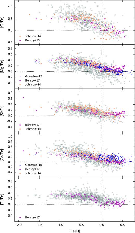
Abundance ratios for the alpha elements from this work (the grey stars) compared to literature studies. The abundance trends derived here are largely in agreement with the literature. In particular, Si, Ca, and Ti seem to follow the same trend and similar abundance scale to the microlensed dwarfs (Bensby et al. 2017). However, for the elements O and Mg, our scatter is considerably larger than other studies. See text for details.
In summary, the alpha abundances derived in this work follow the same trend as some of the most recent, high signal-to-noise, high-resolution studies of bulge stars. For oxygen and magnesium, our results show considerably larger scatter (approximately twice) compared to literature studies, and an offset in the mean magnesium abundances. However, [Si/Fe], [Ca/Fe], and [Ti/Fe] show comparable scatter and abundance scale to other studies. For both O and Mg, a plateau can be seen from [Fe/H] ≲ −0.5, and the abundances of both elements decrease as function of [Fe/H] above solar metallicity. Si, Ca, and Ti show similar trends, flattening to near-solar or solar values for [Fe/H] ≥ 0. This behaviour at supersolar metallicity was seen as unique to microlensed bulge dwarfs (e.g. Johnson et al. 2014), however, we confirm that this is not the case. A plateau at [X/Fe] ≈ 0.3 dex can be seen for Si and Ti, from [Fe/H] ≲ −0.5. Finally, although the abundance trends are largely consistent with the literature, there are some inconsistencies in terms of abundance scale at different metallicity regimes.
7.1 Variation with latitude
As the contribution of metallicity components change with latitude, such that the metal-rich component dominates near the plane, one would expect a vertical gradient in [α/Fe] in the opposite sense: that the low-α population dominates near the plane, and the high-α population dominates away from the plane. This has been observed by Gonzalez et al. (2011) for their bulge giants located near the minor axis, at Baade’s window and (ℓ, b) = (0.21, −6) and (0, −12). More recently, Fragkoudi et al. (2018) showed that a positive [α/Fe] gradient is also present in their N-body simulation, where the bulge population originated from three disc components.
The same conclusion can be drawn from Fig. 8, which shows the distribution of [α/Fe] for bulge fields observed in this work. We used the weighted average of the elements Mg, Si, Ca, and Ti to determine [α/Fe]. Oxygen was excluded because it may have a different chemical evolution history to the other alpha elements, as discussed in the previous section. The weighted average [α/Fe] is mostly influenced by Si and Ti, which are the most precisely measured elements. We do not report [α/Fe] values for [Fe/H] < −1.5 because most of the elemental abundances cannot be measured at this metallicity regime.
![Left-hand panel: the weighted average of Mg, Si, Ca, and Ti ([α/Fe]) as a function of [Fe/H] for the three minor axis fields. Right-hand panel: the corresponding histograms of [α/Fe] at different latitudes. The mean [α/Fe] values and standard deviations are given for each field. Overall [α/Fe] increases with latitude, but the dispersion seems to be smaller at the highest latitude (b = −10).](https://oup.silverchair-cdn.com/oup/backfile/Content_public/Journal/mnras/486/3/10.1093_mnras_stz1104/1/m_stz1104fig8.jpeg?Expires=1750427786&Signature=vdgqQTFLI-mjIh0~B5gZlXPVrmQP5pTQE9uPWovo5PXY-Sbzaj1m4rjzfiouUmRtSrpiJnbFK94hutCP-5kDR~FARKP0hBP6F20lLHfUGFFM9cHO2D1a7eVY5U-NQD6aFkASScskCW01koY8Z5b6nIO55IXcfHTeL08Qoo8YTBq~Y0-tvBHzGw0nKzmMu9qOJMS170IvtOfjh9PCm9OhvQ5ofpOr6COmfeRqEgwZxl61tNwYknt9mGywU~1pgb6mx9JtBdy-7nyv40jnw-62vcsf2TCS1LEe8AFvkHOfBXZBVHOeGmpuqoKdapM~FEZ-ZGVl2V7RkCbKu7YgfZPRbw__&Key-Pair-Id=APKAIE5G5CRDK6RD3PGA)
Left-hand panel: the weighted average of Mg, Si, Ca, and Ti ([α/Fe]) as a function of [Fe/H] for the three minor axis fields. Right-hand panel: the corresponding histograms of [α/Fe] at different latitudes. The mean [α/Fe] values and standard deviations are given for each field. Overall [α/Fe] increases with latitude, but the dispersion seems to be smaller at the highest latitude (b = −10).
We observe that the mean [α/Fe] indeed shifts towards higher values at higher latitudes. However, the median value and shape of [α/Fe] changes sharply between b = −5° and b = −7.5°. Closer to the plane, the distribution is fairly uniform, but away from the plane, it is positively skewed (towards higher [α/Fe] values). The alpha abundance distributions of b = −7.5° and b = −10° are similar in shape and mean value, however, b = −7.5° have slightly larger dispersion. These observations can be explained by the relative contributions of different metallicity components observed by ARGOS: the fraction of the most metal-rich (low-α) component drops significantly between b = −5° and b = −7.5°, whereas the component contributions are similar for fields b = −7.5° and b = −10° (Ness et al. 2013b). Qualitatively, our results are consistent with that of Gonzalez et al. (2011; see their fig. 15), although our MDF is biased, which could affect the [α/Fe] distribution function. An interesting point to note is that there is a hint of decreasing σ[α/Fe] as a function of latitude, which can also be seen for southern APOGEE bulge fields near the minor axis (see fig. 12, Fragkoudi et al. 2018).
While an increase in the mean [α/Fe] with distance from the plane is expected (Gonzalez et al. 2011; Fragkoudi et al. 2018), intrinsic vertical abundance gradients of the different bulge metallicity components have not been established. In this work we are well placed to assess the variation with latitude (if any) of each metallicity component, as we have sampled the same range of metallicity at each latitude. For some elements, we are able to measure abundances down to [Fe/H] ≈ −2, but for most elements (and thus [α/Fe]), we are able to probe metallicity components within −1.5 ≲ [Fe/H] ≲ 0.5.
For each latitude, we computed the median [α/Fe] at different [Fe/H] bins, in steps of 0.2 dex, shown in Fig. 9. Errors in the median [α/Fe] values are computed as the standard error in the mean. Given the uncertainties, we do not observe variations in alpha abundances across the latitude range covered here for −1 < [Fe/H] < 0. Similarly, Ryde et al. (2016) did not find vertical variations in the alpha abundances of inner bulge stars within 2° from the Galactic plane. At the low-metallicity regime ([Fe/H] < −1), variations between fields (0, −7.5) and (0, −10) can be seen for certain elements (O, Mg, and Si). However, the trends are not consistent. These differences more likely caused by the higher uncertainties in abundance measurements and smaller samples for [Fe/H] < −1. At the metal-rich regime ([Fe/H] > 0), for all alpha elements except calcium, the abundances of field (0, −10) are enhanced compared to field (0, −5). This can be seen most clearly for [α/Fe], but is much less certain for [O/Fe]. We note, however, that there are fewer stars at the high-metallicity regime, especially for field (0, −10).
![The median trends of each α-element, and the weighted average [α/Fe] at different latitudes. Median points are computed for [Fe/H] bins of ≈0.2 dex in width. The error bars are the standard deviation in the mean.](https://oup.silverchair-cdn.com/oup/backfile/Content_public/Journal/mnras/486/3/10.1093_mnras_stz1104/1/m_stz1104fig9.jpeg?Expires=1750427786&Signature=0kJ823~uTPg10N1UUkRFj1~1RIpFV8~RPLnzM6pLHCjInPTYW7sAHAI8saz~ANPQqeikGCZBsm7dx8pNdjG03eS4OwkfuAmr0pRqqaEakj15xog2xauHYh5DRH9tk8NYfbKN02Yt4Ub4T70UXbsAOdE1Hkcfzg0Dji33N91atsPjH0FeABcr7deDu~g5ORntOPUGyBB7EBIHmPrNTPl2PY0zxpXhOIroThUIH2J4hbvOFEnWNICXSMkxWOkR43NnBjyVSiJx9tfzQRG1EKzAwUxnGC1MI2eQUToigxP-20kA8PZYFPKgyYDmoy6arbnddFRSfPk8ZTTpU137kZYxJQ__&Key-Pair-Id=APKAIE5G5CRDK6RD3PGA)
The median trends of each α-element, and the weighted average [α/Fe] at different latitudes. Median points are computed for [Fe/H] bins of ≈0.2 dex in width. The error bars are the standard deviation in the mean.
The lack of vertical alpha abundance gradient in each metallicity component for [Fe/H] < 0 is indicative of fast bulge evolution. Similarly, it has been shown that the high-α disc population (commonly referred to as the thick disc) does not exhibit a vertical [α/Fe] gradient (Ruchti et al. 2011; Mikolaitis et al. 2014; Duong et al. 2018).
7.2 Comparison with GALAH DR2
Because this work uses the same lines, atomic data and spectral analysis technique as the GALAH survey, systematic differences and offsets are minimal (see Appendix A). Although differences are expected due to our independent reduction and lower S/N, our bulge sample allows for a consistent comparison with disc/halo stars from the GALAH survey DR2 (Buder et al. 2018). To avoid intrinsic offsets in the abundance ratios of different stellar types, we restricted the GALAH sample to approximately the same parameters space as that shown in Fig. 3: Teff ≈ 4000–5000 K and log g ≈ 3.5–1.5 cm s−2. For a fair comparison, we only used results determined by sme, i.e. the reference results used to train The Cannon. The GALAH training set is of high fidelity and signal to noise, with mean SNR of ≈100 per pixel for the green CCD. Due to the survey observing strategy, most GALAH stars are in the outer disc. Assuming R⊙ = 8 kpc, over 90 per cent of the comparison sample are located at RGC > 7 kpc and 80 per cent are in the solar neighbourhood (7 < RGC < 9 kpc). The RGC-z distribution of GALAH giants is shown in Fig. 10.
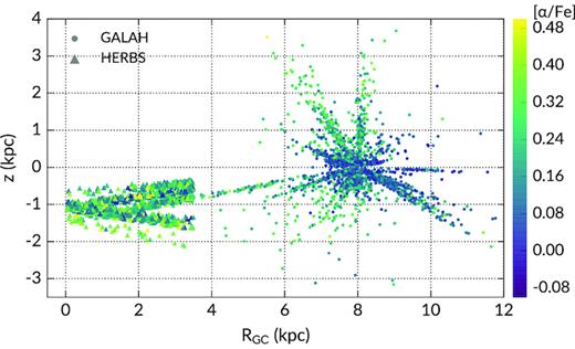
The distribution of HERBS (the triangle) and GALAH (the circle) giants in the RGC-z plane. We assumed R⊙ = 8 kpc. HERBS stars are located near the Galactic centre (RGC < 4 kpc) and close to the plane. Most of the GALAH stars are located in the solar neighbourhood due to the survey observing strategy.
We determined the component membership of the GALAH disc stars based on their weighted average [α/Fe], which shows the clearest separation between the disc components. We separated the low and high-α populations of the disc guided by the ‘gap’ in the [α/Fe] distribution. The separation is shown in Fig. 11. At the metal-poor regime ([Fe/H] ≤−1), there is substantial overlap between the metal-weak thick disc and halo in velocities, metallicity, and abundances (e.g. Reddy & Lambert 2008). To identify halo stars, we relied on the space velocities U, V, W, computed using Gaia DR2 parallaxes and proper motions (Gaia Collaboration 2016, 2018). The solar motion is corrected by adapting (U, V, W)⊙ = (11.1, 12.24, 7.25) from Schönrich, Binney & Dehnen (2010). Fig. 11 shows the total velocity |$V_\mathrm{tot} \equiv \sqrt{\strut U^2 + V^2 + W^2}$| as a function of [Fe/H]. We designated those with Vtot > 180 km s−1 as likely halo stars (e.g. Nissen & Schuster 2010).
![Definitions of stellar populations in the GALAH sample. Left-hand panel: Vtot as a function of metallicity. The dotted line shows Vtot = 180 km s−1, which separates the halo from the disc components. Right-hand panel: The [α/Fe] distribution of GALAH disc stars; stars above the dashed line is defined as the high-α population, and below the dashed line is the low-α population. The large stars indicate the halo population (Vtot > 180 km s−1).](https://oup.silverchair-cdn.com/oup/backfile/Content_public/Journal/mnras/486/3/10.1093_mnras_stz1104/1/m_stz1104fig11.jpeg?Expires=1750427786&Signature=FeFRd1KUgj2Q2Cg9NMlnARVyTBleuD49kP9GrLs7jHhyedlnGrx6acGliXXqFFN0JTS34MpXTfAz10hM7evXk2ohECPAoyFK0r8faqpmurtcZxTT2J~NM1gLCUlEk3mmT95mdcIm9Apk33X~4nOSsrE4AMBxMSGVJ~7amycNEa3PsTITrNKLLbX4p~TD5Ngs9IolvTvFyCBc4MEGe5pPFmC0mOC46gosm2aDbICJLBy1VgPILXUILuNSukIPl6ZKd~EjgUqnlP8u5fx0U4LNZrxfL4PtaOp9lGH2jpxKXJkzpfB0fONej6nBE1lOjryHgizyEk5QX4bnGMoJ9c9PBA__&Key-Pair-Id=APKAIE5G5CRDK6RD3PGA)
Definitions of stellar populations in the GALAH sample. Left-hand panel: Vtot as a function of metallicity. The dotted line shows Vtot = 180 km s−1, which separates the halo from the disc components. Right-hand panel: The [α/Fe] distribution of GALAH disc stars; stars above the dashed line is defined as the high-α population, and below the dashed line is the low-α population. The large stars indicate the halo population (Vtot > 180 km s−1).
Fig. 12 shows the comparison of bulge and disc/halo abundance trends for the five alpha elements and weighted average [α/Fe]. Our abundance trends and scale are mostly compatible with GALAH, as we would expect. We note that our [Mg/Fe] trend does not resemble the GALAH trend as do the other elements. This may be due to the different Mg lines used in this study and GALAH (we omitted a magnesium line at 4730 Å due to blending). For this reason, we do not show the comparison for [α/Fe], as this average would be affected by the systematic difference between our and GALAH [Mg/Fe] ratios.
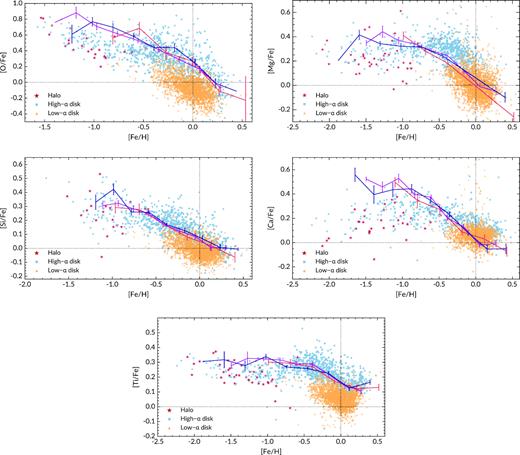
Comparison of the abundance trends in the Galactic bulge and disc/halo. The data points are training set giants from GALAH DR2, separated into the disc and halo components as described in the text. The solid lines are median abundance trends of three bulge fields along the minor axis (colours have the same meaning as in Fig. 9).
Overall, the bulge trend follows that of the high-α disc component for [Fe/H] ≳ − 0.8. The bulge abundances remain enhanced compared to the low-α component also at the metal-rich regime. However, both Mg and Ca abundance ratios show little difference between the low-α disc and bulge, especially at high metallicity. We note the high and low-α discs are not easily separated in the GALAH [Mg/Fe] and [Ca/Fe] distributions, perhaps due to the lower precision of these measurements (see Buder et al. 2018 for details). Except for Mg and Ca, the rest of the alpha elements (O, Si, Ti) show behaviours that are in line with the conclusion of many previous works: that the bulge and high-α disc population shares a similar chemical evolution (Meléndez et al. 2008; Alves-Brito et al. 2010; Johnson et al. 2014; Bensby et al. 2017; Jönsson et al. 2017; Rojas-Arriagada et al. 2017). There is thus good evidence to support a disc origin for bulge stars with [Fe/H] > −0.8. We note that McWilliam (2016) concluded the bulge is enhanced in [Mg/Fe] compared to the thick disc by examining several literature studies, however, this comparison may be affected by systematic offsets between bulge red giant branch (RGB) and thick disc main-sequence stars.
The metal-poor bulge population ([Fe/H] ≲ −0.8), however, appears to be enhanced in some alpha elements compared to the thick disc and halo by ≈0.1 dex. This result is less conclusive for [Si/Fe], where the scatter at low metallicity is higher than other elements.
The enhanced alpha abundance ratios suggest a slightly higher star formation rate for the metal-poor bulge population, as the initial mass function of the bulge has shown to be consistent with that of the local disc (e.g. Calamida et al. 2015; Wegg, Gerhard & Portail 2017). The metal-poor bulge population also has distinctive kinematics signatures: Ness et al. (2013b) found that stars with [Fe/H] < −1 have a different rotation profile to the metal-rich stars, and Zoccali et al. (2017) showed that their metal-poor bulge stars rotate more slowly. This would suggest that the metal-poor population may not share the same disc origin as the more metal-rich populations.
8 CONCLUSIONS
In this work, we have successfully obtained stellar parameters and α-element abundances for 832 RGB stars at latitudes b = −5°, −7.5°, −10° along the minor axis of the Galactic bulge. The majority of our sample are ARGOS survey stars with predetermined bulge memberships. ARGOS stars were selected based on metallicity, so that we observe higher relative fractions of the metal-rich and metal-poor bulge populations.
According to our analysis of stars in common with ARGOS, the metallicity scale reported by Ness et al. (2013a) should be compressed, i.e. we obtain slightly higher [Fe/H] for metal-poor ARGOS stars, and vice versa. Our results suggest that along the minor axis, the spacing between ARGOS MDF component centroids should be ≈0.09 dex closer. The effect of this is most apparent in field (0, −7.5), where primary ARGOS components A and B become almost indistinguishable. However, the ARGOS components remain distinct (given measured ARGOS dispersions) for fields (0, −5) and (0, −10).
The optical wavelength range and resolving power of the HERMES spectrograph allowed us to measure chemical abundances for up to 28 elements, including the alpha elements O, Mg, Si, Ca, and Ti. In general, we find that the [X/Fe] versus [Fe/H] trends of these elements follow that of previous works at similar resolving power. We also observe similar trends to the microlensed dwarfs sample from Bensby et al. (2017), which was observed at much higher resolving power but is limited to less than 100 stars. Within the scatter of the data sets, we confirm that there are no significant systematic differences between the bulge giants and microlensed dwarfs, except for [Ca/Fe] from [Fe/H] < −0.5, where our median [Ca/Fe] is higher by up to 0.2 dex. In addition, our [Mg/Fe] values decrease as a function of [Fe/H] and do not flatten at supersolar metallicity. We find that the mean value of [α/Fe] increases with increasing distance from the plane, which is expected as the metal-poor component dominates at high latitudes. We also find that the [α/Fe] dispersion is smaller at higher latitudes.
Our metallicity coverage allowed us to assess the vertical variation in alpha abundances of the different bulge metallicity components. Within uncertainties, the abundance ratios remain uniform with height for most metallicity bins. At the metal-rich regime ([Fe/H] > 0), there is evidence of enhanced alpha-abundances in field (0, −10), which is most conclusive for [α/Fe] (weighted average of Mg, Ca, Si, Ti). However, this conclusion is more uncertain for individual elements, and does not seem to hold true for [Ca/Fe]. The bulge abundance trends appear to follow that of the high-α disc population, and are enhanced compared to the low-α disc population at supersolar metallicities. However, the more metal-poor bulge population ([Fe/H] ≲ −0.8) is enhanced compared to thick disc and halo stars at the same metallicity.
The lack of vertical abundance variation for different metallicity components and abundance trends similar to the high-α, or thick disc population, both point to fast chemical enrichment in the bulge (e.g. Friaça & Barbuy 2017). Furthermore, the metal-poor bulge population may have experienced a different evolution, as we observe that it is enhanced in alpha abundances compared to the high-α disc population. This may be compatible with previous findings that the metal-poor population has distinct kinematics compared to the metal-rich population, and indicates that the bulge does not just consist of stars originating from the disc. We further explore the chemical evolution of the bulge and its connection to the disc in the next paper of this series, which will focus on the abundances light, iron peak, and heavy elements.
ACKNOWLEDGEMENTS
We thank the anonymous referee for helpful comments that improved this manuscript. LD, MA, and KCF acknowledge funding from the Australian Research Council (projects FL110100012 and DP160103747). LD gratefully acknowledges a scholarship from Zonta International District 24. DMN was supported by the Allan C. and Dorothy H. Davis Fellowship. LMH was supported by the project grant ‘The New Milky Way’ from the Knut and Alice Wallenberg foundation. MA’s work was conducted as part of the research by Australian Research Council Centre of Excellence for All Sky Astrophysics in 3 Dimensions (ASTRO 3D), through project number CE170100013. Part of this research was conducted at the Munich Institute for Astro- and Particle Physics of the DFG cluster of excellence ‘Origin and Structure of the Universe’. This publication uses data products from the Two Micron All Sky Survey, which is a joint project of the University of Massachusetts and the Infrared Processing and Analysis Center/California Institute of Technology, funded by the National Aeronautics and Space Administration and the National Science Foundation. We acknowledge the use of data from the European Space Agency (ESA) mission Gaia (https://www.cosmos.esa.int/gaia), processed by the Gaia Data Processing and Analysis Consortium (DPAC, https://www.cosmos.esa.int/web/gaia/dpac/consortium). Funding for the DPAC has been provided by national institutions, in particular the institutions participating in the Gaia Multilateral Agreement. The GALAH survey is based on observations made at the Australian Astronomical Observatory, under programmes A/2013B/13, A/2014A/25, A/2015A/19, A/2017A/18. We acknowledge the traditional owners of the land on which the AAT stands, the Gamilaraay people, and pay our respects to elders past and present.
Footnotes
Despite the overall small fraction of young stars in the bulge, Bernard et al. (2018) found a significant fraction (30–40 per cent) of supersolar metallicity stars to be younger than 5 Gyr. Bensby et al. (2013) and Haywood et al. (2016) also discussed the possibility of young stars masquerading as an old turn-off in colour–magnitude diagrams due to a lack of metallicity information in photometric studies.
Barbuy et al. (2018) argued that due to large uncertainties in the distances of microlensed dwarfs, at least some of these young stars are not part of the bulge, but foreground disc stars.
See Lee, Joo & Chung (2015) and Joo, Lee & Chung (2017) for a different interpretation of the double red clump in relation to the X-shaped morphology of the Galactic bulge. In addition, López-Corredoira (2016, 2017) observed an absence of the X-structure in the young, main-sequence bulge population and Mira variables.
The [M/H], or metallicity parameter is the iron abundance of the best-fitting model atmosphere. In our case, this value is very close to the true iron abundance derived from iron lines only. For the purpose of notation consistency when comparing with other studies, we refer to [M/H] as [Fe/H] in subsequent sections.
It made little difference to [O/Fe] whether we use all three lines of the oxygen triplet, or just the 7772 Å line. As the other two lines of the triplet are significantly weaker (therefore often undetectable) in our spectra, we chose to use only the 7772 Å line.
The biases are defined as the median of the difference (sme − benchmark).
REFERENCES
APPENDIX A: SPECTROSCOPIC ANALYSIS TESTS
A1 Benchmark stellar parameters comparison
To estimate the accuracy of our stellar parameters, we analysed giants and subgiants in the Gaia benchmark stars (GBS) sample (giants only) using the reduction and parameter optimization pipeline described above. For this purpose, we used archive HERMES benchmark observations that were taken for the GALAH survey. To gauge the effects of the difference in reduction methods between our survey (2dfdr-based) and the GALAH survey (iraf-based), we also compared our benchmark results with that obtained from spectra reduced with the GALAH reduction pipeline. The results are shown in Fig. A1. We note that the GALAH spectrum of the benchmark giant ϵFor was not available, but this star is included in the 2dfdr comparison sample. We performed our analysis assuming |$\mathcal {R}$| = 28 000. For the iraf benchmark reductions, adopting either this constant spectral resolution or the resolution map from Kos et al. (2017) returned near-identical results, with temperature differences ≤30 K, metallicity differences ≤0.04 dex, and surface gravity differences ≤0.1 dex, all within expected uncertainties.
![Comparison of sme-derived parameters with fundamental Teff, log g (Heiter et al. 2015b), and Gaia ESO-derived [Fe/H] (from high-resolution UVES spectra, Jofré et al. 2014) for benchmark stars. The squares indicate 2dfdr-based reductions and the circles are results from iraf-based reductions. The differences are shown as (sme − GBS); the red line indicates biases for 2dfdr-based reductions only. The outlier in log g is the M-giant αCeti.](https://oup.silverchair-cdn.com/oup/backfile/Content_public/Journal/mnras/486/3/10.1093_mnras_stz1104/1/m_stz1104figa1.jpeg?Expires=1750427786&Signature=ol2jJ7uddTahkfUxW6bNqpRDEgplHZou5wK3TbJkNh537uUnfmwWwUu1NCxMl6MX1voAA8RhpEwFY2JnDWggLDGZFCyaFuIYpr55r2qsfQ-Y~U8FlmOigctCPAj6ZulpmuZ59z-BEa1mZDdcBMzgEHnlaN8baY2kN2jmBmDIoSo5IyLX2nWnaTu79W73oNtRdrwjYIgYkxCQkDon8ze8zAciFtkOhC5o0iDULShMBZxvnwfk04PP4etwXWtAig4hGX5L6fvqIImbPGvp3IJLr6uRF1rOfu1Zm8pAN3bB5ltIDMBCGRA0WiTU0jrDkBnx6LVtY218WXcpX0tUapKCpQ__&Key-Pair-Id=APKAIE5G5CRDK6RD3PGA)
Comparison of sme-derived parameters with fundamental Teff, log g (Heiter et al. 2015b), and Gaia ESO-derived [Fe/H] (from high-resolution UVES spectra, Jofré et al. 2014) for benchmark stars. The squares indicate 2dfdr-based reductions and the circles are results from iraf-based reductions. The differences are shown as (sme − GBS); the red line indicates biases for 2dfdr-based reductions only. The outlier in log g is the M-giant αCeti.
In general, the differences between the two reduction methods are not significant. For the 2dfdr sample, we observe biases8 and standard deviations for Teff: 40 ± 90 K; log g: 0.02 ± 0.25 dex, and [Fe/H]: −0.12 ± 0.08 dex. The iraf biases and standard deviations for Teff, log g, and [Fe/H] are 100 ± 90 K, −0.06 ± 0.22 dex, and −0.05 ± 0.06 dex, respectively. While both sets of results are fairly accurate, spectra from the GALAH reduction pipeline produce slightly more precise log g and [Fe/H], perhaps due to the tilted PSF correction that increases the resolution and signal to noise towards the CCD corners. However, GALAH-reduced spectra return even higher effective temperature for giants compared to our reductions, which already overestimates Teff by 40 K compared to reference values.
For the GALAH reductions, the biases of this giants-only sample is different to that of the full giants and dwarfs benchmark sample analysed by Sharma et al. (2018). Before bias correction, Sharma et al. (2018) quoted biases in Teff: 23 ± 112 K, log g: −0.15 ± 0.22 dex, and [Fe/H]: −0.12 ± 0.1 dex. Here, we find that neither log g nor [Fe/H] shows a strong offset, and the metallicity precision is higher compared to the full sample.
We derived particularly discrepant surface gravity results for the M-giant αCeti. Compared to the benchmark value from Heiter et al. (2015b), this star has Δlog g = 1 dex, for both 2dfdr and iraf reductions. The cause of this discrepancy is unclear, seeing as the M-giant αTau with similar parameters does not show this large deviation. This may be a concern that surface gravity determination for log g < 1 dex is challenging with HERMES spectra. The outlier αCeti has been excluded from log g standard deviation calculations. Another notable discrepant point is the cool giant HD107328, with Δlog g = −0.56. Buder et al. (2018) showed that a result close to the GBS value can only be produced if Gaia DR1 parallax is used. This indicates there are some difficulties in analysing line-rich stars with our spectroscopic method and wavelength region.
Our comparison here shows that 2dfdr-reduced spectra perform just as well as iraf-reduced spectra, however, the iraf reductions return higher precision for [Fe/H] and log g. We do not see significant biases in effective temperature or surface gravity in our results, and thus do make corrections to these parameters. However, the metallicity is underestimated by our pipeline by −0.12 dex. Similar to GALAH, we corrected for this metallicity bias by adding +0.1 dex to all of our [Fe/H] values.
A2 Abundance trends with temperature
Fig. A2 shows the abundance-temperature trends for each α-element. We do not observe correlations for oxygen, silicon, and titanium. [Mg/Fe] and [Ca/Fe] both show positive linear trends with respect to temperature. For calcium, this could be due to non-LTE effects, however, the reason for the [Mg/Fe]–Teff correlation is not clear. The non-LTE magnesium abundances of M67 giants observed by GALAH also the same trend with temperature (see Gao et al. 2018, their fig. 7).
![Abundance-temperature trends for the alpha elements; the red dashed lines are running medians over four metallicity bins. We do not see obvious correlations in [O/Fe], [Si/Fe], and [Ti/Fe]. Similar linear trends are observed for [Mg/Fe] and [Ca/Fe].](https://oup.silverchair-cdn.com/oup/backfile/Content_public/Journal/mnras/486/3/10.1093_mnras_stz1104/1/m_stz1104figa2.jpeg?Expires=1750427786&Signature=Cc8O0hHBzuSgmsPN4tS4idpMclUYk1bHsmp4Sdb29BFPxg-QwOH8YrIHknKy00B3JdH2ia5VfBVP7AyKyuzRPrg1oQ0AO-b2C7FaKHln9HX1GulWiwx2l66drgy6vOagPCC9qH1cOBN0KdaAZQ-aso3ribyMZ1zDdZRG~CjfkxRnIhToo8fv5wEEn4umyn8LO89-GTnz8BG4u8D8yNz-asJk7XZbIzlJdlw0SG5yV0FaJLQZq-XfFcs2uUaa08-ivoOoCCr~1rxpav2DzEY0R-28ukI4cX9K8MIGn08SkIN16hxNiY0nySrqSUwmlh-vShf3pfgbESFs0SCIhAgSrA__&Key-Pair-Id=APKAIE5G5CRDK6RD3PGA)
Abundance-temperature trends for the alpha elements; the red dashed lines are running medians over four metallicity bins. We do not see obvious correlations in [O/Fe], [Si/Fe], and [Ti/Fe]. Similar linear trends are observed for [Mg/Fe] and [Ca/Fe].
APPENDIX B: DATA TABLES
The catalogue containing stellar parameters, abundance ratios, and their uncertainties is provided as online supporting material, accessible through the publisher website. The contents of the catalogue are described in Table B1. We also provide the list of lines used for stellar parameters and abundance analysis in Tables B2 and B3. The atomic data and lines used for stellar parameters analysis are the same as that of the GALAH survey (Buder et al. 2018). Except for Ti, we did not use all of the lines available in the GALAH linelist for abundance analysis.
Description of the data catalogue. The uncertainties in abundance ratios are χ2 fitting errors; the uncertainties in stellar parameters are χ2 fitting errors and standard deviations from Fig. A1 added in quadrature.
| Column | Name | Description |
|---|---|---|
| [1] | 2MASS ID | The 2MASS identifier of the star |
| [2] | RAJ2000 | The right ascension at epoch J2000 (°) |
| [3] | DECJ2000 | The declination at epoch J2000 (°) |
| [4] | Teff | Effective temperature (K) |
| [5] | |$\sigma _\mathrm{T_{eff}}$| | Uncertainty in effective temperature (K) |
| [6] | log g | Surface gravity (cm s−2) |
| [7] | σlog g | Uncertainty in surface gravity (cm s−2) |
| [8] | [Fe/H] | Metallicity |
| [9] | σ[Fe/H] | Uncertainty in metallicity |
| [10] | [O/Fe] | Abundance ratio for O |
| [11] | σ[O/Fe] | Uncertainty in [O/Fe] |
| [12] | [X/Fe] | Same as [10], but for Mg |
| [13] | σ[X/Fe] | Same as [11], but for Mg |
| [14] | [X/Fe] | Same as [10], but for Si |
| [15] | σ[X/Fe] | Same as [11], but for Si |
| [16] | [X/Fe] | Same as [10], but for Ca |
| [17] | σ[X/Fe] | Same as [11], but for Ca |
| [18] | [X/Fe] | Same as [10], but for Ti |
| [19] | σ[X/Fe] | Same as [11], but for Ti |
| [20] | ARGOS Teff | ARGOS effective temperature (K) |
| [21] | ARGOS log g | ARGOS surface gravity (cm s−2) |
| [22] | ARGOS [Fe/H] | ARGOS metallicity |
Line data used for stellar parameters determination, common to this work, and GALAH DR2.
| Species | Wavelength (Å) | log (gf) | Excitation potential (eV) | Species | Wavelength (Å) | log (gf) | Excitation potential (eV) |
|---|---|---|---|---|---|---|---|
| Sc i | 4743.8300 | 0.422 | 1.448 | Fe i | 5661.3447 | −1.756 | 4.284 |
| Sc i | 4753.1610 | −1.659 | 0.000 | Fe i | 5662.5161 | −0.447 | 4.178 |
| Sc i | 5671.8163 | −0.290 | 1.448 | Fe i | 5679.0229 | −0.820 | 4.652 |
| Sc i | 5686.8386 | −0.133 | 1.440 | Fe i | 5680.2404 | −2.480 | 4.186 |
| Sc i | 5717.3070 | −0.532 | 1.440 | Fe i | 5696.0892 | −1.720 | 4.549 |
| Sc i | 5724.1070 | −0.661 | 1.433 | Fe i | 5701.5442 | −2.193 | 2.559 |
| Sc ii | 5657.8960 | −0.603 | 1.507 | Fe i | 5705.4642 | −1.355 | 4.301 |
| Sc ii | 5667.1490 | −1.309 | 1.500 | Fe i | 5731.7618 | −1.200 | 4.256 |
| Sc ii | 5684.2020 | −1.074 | 1.507 | Fe i | 5732.2960 | −1.460 | 4.991 |
| Sc ii | 6604.6010 | −1.309 | 1.357 | Fe i | 5741.8477 | −1.672 | 4.256 |
| Sc ii | 5669.0420 | −1.200 | 1.500 | Fe i | 5775.0805 | −1.080 | 4.220 |
| Ti i | 4758.1178 | 0.510 | 2.249 | Fe i | 5778.4533 | −3.430 | 2.588 |
| Ti i | 4759.2697 | 0.590 | 2.256 | Fe i | 5806.7249 | −0.950 | 4.608 |
| Ti i | 4778.2547 | −0.350 | 2.236 | Fe i | 5809.2174 | −1.740 | 3.884 |
| Ti i | 4781.7106 | −1.950 | 0.848 | Fe i | 5811.9144 | −2.330 | 4.143 |
| Ti i | 4797.9757 | −0.630 | 2.334 | Fe i | 5814.8071 | −1.870 | 4.283 |
| Ti i | 4801.9016 | −3.060 | 0.818 | Fe i | 5849.6833 | −2.890 | 3.695 |
| Ti i | 4820.4094 | −0.380 | 1.503 | Fe i | 5853.1483 | −5.180 | 1.485 |
| Ti i | 5689.4600 | −0.360 | 2.297 | Fe i | 5855.0758 | −1.478 | 4.608 |
| Ti i | 5716.4500 | −0.720 | 2.297 | Fe i | 5858.7780 | −2.160 | 4.220 |
| Ti i | 5720.4359 | −0.900 | 2.292 | Fe i | 6481.8698 | −2.981 | 2.279 |
| Ti i | 5739.4690 | −0.610 | 2.249 | Fe i | 6494.9804 | −1.268 | 2.404 |
| Ti i | 5866.4513 | −0.790 | 1.067 | Fe i | 6498.9383 | −4.687 | 0.958 |
| Ti i | 6716.6660 | −1.370 | 2.488 | Fe i | 6546.2381 | −1.536 | 2.759 |
| Ti ii | 4719.5109 | −3.320 | 1.243 | Fe i | 6592.9124 | −1.473 | 2.728 |
| Ti ii | 4764.5247 | −2.690 | 1.237 | Fe i | 6593.8695 | −2.420 | 2.433 |
| Ti ii | 4798.5313 | −2.660 | 1.080 | Fe i | 6597.5592 | −0.970 | 4.795 |
| Ti ii | 4849.1678 | −2.960 | 1.131 | Fe i | 6609.1097 | −2.691 | 2.559 |
| Ti ii | 4865.6104 | −2.700 | 1.116 | Fe i | 6627.5438 | −1.590 | 4.549 |
| Ti ii | 4874.0094 | −0.860 | 3.095 | Fe i | 6648.0796 | −5.918 | 1.011 |
| Fe i | 4788.7566 | −1.763 | 3.237 | Fe i | 6677.9851 | −1.418 | 2.692 |
| Fe i | 4793.9614 | −3.430 | 3.047 | Fe i | 6699.1413 | −2.101 | 4.593 |
| Fe i | 4794.3541 | −3.950 | 2.424 | Fe i | 6703.5660 | −3.060 | 2.759 |
| Fe i | 4802.8797 | −1.510 | 3.642 | Fe i | 6713.7425 | −1.500 | 4.795 |
| Fe i | 4808.1478 | −2.690 | 3.251 | Fe i | 6725.3558 | −2.100 | 4.103 |
| Fe i | 4875.8770 | −1.900 | 3.332 | Fe i | 6733.1503 | −1.480 | 4.638 |
| Fe i | 4890.7551 | −0.386 | 2.876 | Fe ii | 4720.1386 | −4.480 | 3.197 |
| Fe i | 4891.4921 | −0.111 | 2.851 | Fe ii | 4731.4476 | −3.100 | 2.891 |
| Fe i | 5651.4689 | −1.900 | 4.473 | Fe ii | 4833.1916 | −5.110 | 2.657 |
| Fe i | 5652.3176 | −1.850 | 4.260 |
Line data used for abundance determination. The same Ti lines in Table B2 were used to determine [Ti/Fe].
| Species | Wavelength (Å) | log (gf) | Excitation potential (eV) | Species | Wavelength (Å) | log (gf) | Excitation potential (eV) |
|---|---|---|---|---|---|---|---|
| O i | 7771.9440 | 0.369 | 9.146 | Si i | 5793.0726 | −1.963 | 4.930 |
| Mg i | 5711.0880 | −1.724 | 4.346 | Si i | 5701.1040 | −1.953 | 4.930 |
| Mg i | 7691.5500 | −0.783 | 5.753 | Ca i | 5867.5620 | −1.570 | 2.933 |
| Si i | 5690.4250 | −1.773 | 4.930 | Ca i | 6499.6500 | −0.818 | 2.523 |
