


ABSTRACT
We present the results from a systematic search and characterization of ionized outflows in nearby galaxies using the data from the second Data Release of the Mapping Nearby Galaxies at Arecibo Point Observatory (MaNGA) Survey (DR2; >2700 galaxies, z ≤ 0.015). Using the spatially resolved spectral information provided by the MANGA data, we have identified ∼5200 H α-emitting regions across the galaxies and searched for signatures of ionized outflows. We find evidence for ionized outflows in 105 regions from 103 galaxies, roughly 7 per cent of all the H α-emitting galaxies identified in this work. Most of the outflows are nuclear, with only two cases detected in off-nuclear regions. Our analysis allows us to study ionized outflows in individual regions with star formation rates (SFRs) down to ∼0.01 M⊙ yr−1, extending the ranges probed by previous works. The kinematics of the outflowing gas is strongly linked to the type of ionization mechanism: regions characterized by low-ionization emission region emission (LIER) host the outflows with more extreme kinematics (FWHMbroad ∼ 900 km s−1), followed by those originated in active galactic nuclei (550 km s−1), ‘Intermediate’ (450 km s−1), and star-forming (350 km s−1) regions. Moreover, in most of the outflows we find evidence for gas ionized by shocks. We find a trend for higher outflow kinematics towards larger stellar masses of the host galaxies but no significant variation as a function of star formation properties within the SFR regime we probe (∼0.01–10 M⊙ yr−1). Our results also show that the fraction of outflowing gas that can escape from galaxies decreases towards higher dynamical masses, contributing to the preservation of the mass–metallicity relation by regulating the amount of metals in galaxies. Finally, assuming that the extensions of the outflows are significantly larger than the individual star-forming regions, as found in previous works, our results also support the presence of star formation within ionized outflows, as recently reported by Maiolino et al. (2017) and Gallagher et al. (2018).
1 INTRODUCTION
The evolutionary path of galaxies through cosmic time is strongly marked by the availability of gas reservoirs that serve as fuel to perpetuate the formation of new stars and the feeding of their central supermassive black holes. However, these gas reservoirs are sensitive to the influence of feedback from supernovae explosions, stellar winds, or active galactic nuclei (AGN) that can have a severe impact in the gas, mixing and/or heating it up, or even expelling it from the galaxy. Moreover, the star formation activity can be reduced or halted, preventing the formation of new stars and the subsequent stellar mass growth of galaxies (Veilleux, Cecil & Bland-Hawthorn 2005; Heckman & Borthakur 2016). Such relevant consequences that feedback effects can have in the evolution of galaxies demand a proper understanding of their incidence and properties.
Generally, the study of feedback processes is driven by a two-fold motivation: on the one hand, there is a strong interest in understanding the physics of the feedback phenomenon and its characterization; on the other hand, there is also interest, probably even stronger, in evaluating whether the effects of feedback can help explaining some of the observational results that are still not fully comprehended. For instance, when the effects from supernova, stellar winds, and AGN feedback are included in cosmological simulations, the number of galaxies formed at low and high masses is reduced, alleviating the existent discrepancies between the predicted and observed baryonic mass functions (Benson & Madau 2003; Benson et al. 2003). Apart from halting and/or enhancing star formation activity, feedback-induced galactic outflows might also play an important role in regulating the amount of metals in galaxies (Brooks et al. 2007; Finlator & Dave 2007), contributing to maintaining the relation between the gas-phase metallicity and stellar mass of the galaxies (Tremonti et al. 2004; Mannucci et al. 2010; Dayal, Ferrara & Dunlop 2013; Chisholm, Tremonti & Leitherer 2018). Moreover, the observed metal content of the intergalactic medium (IGM) in high-redshift galaxies could also be explained by the ejection of interstellar material via galactic outflows (Aguirre et al. 2001). Moreover, although feedback processes have been generally invoked as mechanisms that prevent or suppress star formation activity, it has been suggested, first in simulations (Ishibashi & Fabian 2012; Ishibashi, Fabian & Canning 2013) and very recently in observations (Maiolino et al. 2017; Gallagher et al. 2018), that star formation might be triggered inside galactic outflows. Such result would imply the existence of a different mode of star formation, which may play an important role in our understanding of the evolution of galaxies, for instance, contributing to the assembly of stellar mass at high redshift.
The identification of regions in galaxies affected by feedback processes can be done in different ways, including the detection of outflowing gas moving at relatively high velocities with respect to the systemic components (e.g. Westmoquette, Smith & Gallagher 2008), the study of excitation maps of shock-ionized gas (e.g. Veilleux & Rupke 2002), or by exploring their effect on the magnetic fields of galaxies (Damas-Segovia et al. 2016). These outflows have been observed in all gas phases: neutral (Cazzoli et al. 2014; Rubin et al. 2014), molecular (Cicone et al. 2014; Pereira-Santaella et al. 2018), and ionized (Westmoquette et al. 2008; Arribas et al. 2014). The study of galactic outflows has greatly benefitted from the advent of integral field spectroscopic (IFS) instruments, given that they allow spatially resolved studies of the kinematics, ionization mechanisms, morphologies, and physical properties of the outflowing gas across entire galaxies (Bellocchi et al. 2013; Cazzoli et al. 2014). In particular, large IFS surveys such as CALIFA (Sánchez et al. 2012), SAMI (Allen et al. 2015), and MaNGA (Bundy et al. 2015) offer the possibility of exploring the incidence and properties of outflows in a large number of galaxies, allowing a statistically meaningful characterization of such phenomenon.
In this work, we study the incidence and properties of ionized outflows in a large number of galaxies (>2700) observed within the Mapping Nearby Galaxies at Arecibo Point Observatory survey (MaNGA; Bundy et al. 2015) and included in their Data Release 2 (DR2; Abolfathi et al. 2018). This data set includes galaxies with a wide range of stellar masses, star formation rates (SFRs), AGN activity, etc. that allows the characterization of the kinematics and physical properties of the ionized gas in regions hosting ionized outflows. We also investigate the role that outflows might play regulating the star formation activity and metal content of galaxies. A related study on ionized outflows based on the same sample has been recently published by Gallagher et al. (2018), where they focus on the study of star formation taking place within ionized outflows and its implications in galaxy evolution.
In Section 2, we describe the MaNGA DR2 data; Section 3 contains the different steps of our analysis, from the MaNGA datacubes to the spectral modelling of the emission-line spectra; in Section 4 we explain the criteria applied to identify ionized outflows; Section 5 contains the main results from our analysis of the kinematics and properties of the ionized gas, including also discussions about the implications of our results in the context of galaxy evolution; finally, in Section 6 we present the summary and main conclusions of this work. Throughout this work, we adopt a cosmology with H0 = 67.3 km s−1 Mpc−1, ΩM = 0.315, and ΩΛ = 0.685 (Planck Collaboration XVI 2014).
2 DATA SAMPLE
This work is based on data from the DR2 of the MaNGA survey (Abolfathi et al. 2018), one of the three core programs of Sloan Digital Sky Survey IV (SDSS-IV). All the galaxies in the MaNGA sample are part of the main SDSS parent sample and are selected to have stellar masses, M⋆, above 109 M⊙ and redshifts, z, up to 0.15. The spectra span approximately from 3600 to |$10\, 000$| Å, with a spectral resolution that ranges from R ∼ 1400 at 4000 Å to R ∼ 2600 at 9000 Å, corresponding to ∼90 and ∼49 km s−1, respectively. The point spread function (PSF) in the datacubes is 2.5 arcsec (FWHM).
The MaNGA DR2 parent sample is divided into different subsamples. For our analysis, we select all the galaxies that are part of the so-called primary, secondary, and colour-enhanced samples. The two former ones are designed to reach 1.5 Re and 2.5 Re (being Re the effective radius) in |$80{{\ \rm per\ cent}}$| of their targets, respectively, whereas the last one is designed to include underrepresented regions of the M⋆–colour space (see Wake et al. 2017 for more details on the different samples). The combination of these three samples makes up a total of 2672 galaxies. In this work, we use stellar mass estimates, when available, from the SDSS DR7 (Kauffmann et al. 2003b).
3 ANALYSIS
3.1 From datacubes to H α maps
In this work, we use the MaNGA datacubes with linear wavelength sampling (LINCUBE). From the datacubes, we use the 3D flux and inverse variance per unit wavelength, a bad pixel mask, and the spectral resolution as a function of wavelength. Using these data, we generate H α maps for all the galaxies including only the spaxels with S/N > 3 in the H α line, which is estimated as in Rosales-Ortega, Arribas & Colina (2012). In this procedure, we discard all the spaxels where the spectra around the target emission lines are affected by bad pixels. In this way, we generate maps for ∼1500 galaxies showing clear H α emission, roughly 55 per cent of the original MaNGA DR2 sample. An example of one of the H α flux maps generated is shown in Fig. 1.
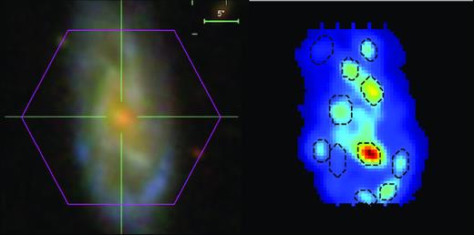
Example of the H α clumps identification in a galaxy. Left: Field of view of MaNGA (the pink hexagon) superimposed on the SDSS coloured image of the galaxy. Right: Map of the H α flux distribution showing the regions identified as H α-emitting clumps.
3.2 Identification of the H α-emitting regions
Once the H α maps are generated and given the clumpy distribution of the H α emission, we develop a method to identify individual regions characterized by H α emission across the galaxies. We note that the corresponding size of the MaNGA PSF in kpc (∼1.5 kpc at the median redshift of the sample, varying from ∼0.6 to ∼6.73 kpc) prevents us from identifying individual star-forming regions, which typically have sizes of 20−100 pc (e.g. Miralles-Caballero, Colina & Arribas 2012). Therefore, the regions identified here probably contain several star-forming regions in most of the cases.
In order to isolate the H α-emitting regions across the MaNGA coverage of the galaxies in an automated way, we start by finding the peaks of emission at different intensity levels using the algorithm clumpfind (Williams, de Geus & Blitz 1994). This algorithm searches for local peaks of emission and follows them down to lower intensity levels, decomposing the H α maps into a set of independent structural units or ‘clumps’ where the emission is concentrated. Once we have identified the H α-emitting regions, we define the sizes of the apertures to extract the spectra by fitting a 2D elliptical isophote with a Gaussian profile. In this procedure, both minor and major axes of the elliptical isophote have to be larger than the FWHM of the MaNGA PSF (2.5 arcsec). For each of the regions, we produce an integrated spectrum by combining all the spaxels with an S/N > 3 in the H α line within the chosen aperture. We do not align the spectra from these spaxels to correct for the systemic velocity of the galaxy in order to preserve the shape of a possible broad component. Finally, given that the MaNGA datacubes do not include covariance calculations, when combining the spectra we calibrate the noise vectors following the recipes from Law et al. (2016). As a result of this analysis, we identify a total of ∼5200 H α-emitting regions across the galaxies, both nuclear and off-nuclear, with a mean of ∼3.5 regions per galaxy.
3.3 Subtraction of stellar component
In order to constrain the kinematics and properties of the ionized gas in the H α-emitting regions, we need to correct their emission-line spectra for the absorption produced by the stellar populations inhabiting them. To do that, we use the software Penalized Pixel-Fitting (ppxf; Cappellari 2017), a tool that models the stellar continuum in the spectra using a maximum penalized likelihood approach. To fit the stellar contribution, we use the PEGASE-HR simple stellar population (SSP) models (Le Borgne et al. 2004), which have the spectral resolution (FWHM ∼ 0.5 Å) and wavelength coverage (3900–6800 Å) appropriate to fit the MaNGA spectra. In this procedure, we take into account the wavelength variation of the spectral resolution in the MaNGA spectra. After fitting the stellar continuum, we subtract it from the galaxies’ spectra to produce pure emission-line spectra. An example of the performance of ppxf is shown in Fig. 2.
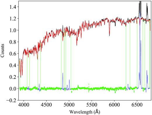
Example of the stellar continuum fit to the spectrum of one of the H α-emitting regions using the software ppxf (Cappellari 2017). The black line corresponds to the observed spectrum, whereas the red line is the best fit to the data. The residuals are shown as a green line and the emission lines, which are masked during the fitting procedure, are shown in blue.
3.4 Spectral fitting
The spectra from regions hosting ionized outflows are characterized by the presence of a secondary, broad kinematic component associated with high gas velocities (see Section 4), superimposed on the systemic emission from the host. When present, this signature is more easily detected in strong emission lines such as H α or |${}[\mathrm{O}\,{\small III}]\, \lambda 5007$|. In these cases, the properties of the outflowing gas can be constrained by fitting the emission-line spectra with a model composed of two Gaussian profiles, corresponding to the narrow (systemic) and broad (outflow) kinematic components. For strong outflows, such as those observed in AGN or starburst galaxies, the broad component can be easily detected and characterized. However, this task becomes significantly more difficult when the outflow is intrinsically weak compared to the total emission from the host region or when the geometry of the outflow or the host galaxy (such as close to edge-on inclinations) hinders the detection of the broad emission. Moreover, since the emission lines associated with the outflow are intrinsically broad, the flux is spread across more spectral pixels and the S/N can be low.
We perform the spectral fitting using a Bayesian approach based on Markov Chain Monte Carlo (MCMC) techniques. In particular, we employ the software developed by Foreman-Mackey et al. (2013), emcee, a tool that implements the Affine Invariant MCMC Ensemble sampler of Goodman & Weare (2010). Using this method, we explore the whole parameter space by sampling more intensively the regions of high likelihood but at the same time allowing the exploration of regions of lower likelihood, preventing in this way the method from getting trapped in regions of local maxima.
For the purpose of our study, we simultaneously fit a model consistent of two sets of Gaussian functions (associated with the narrow and broad kinematic components) to the emission lines H α, H β, |${}[\mathrm{N}\,{\small II}]\, \lambda 6583$|, |${}[\mathrm{O}\,{\small III}]\, \lambda 5007$|, |${}[\mathrm{S}\,{\small II}]$| λλ6717, 6731. In the fitting procedure, we apply the same kinematics (velocity and velocity dispersion) to all the emission lines, fixing the ratio between the two |${}[\mathrm{N}\,{\small II}]$| λλ6548, 6583 lines to 3.06 (Osterbrock 1989). In total, the parameters included in the model are the redshift (z) and width (σ) of each set of Gaussians, the fluxes of each kinematic component in the six spectral lines and the continuum around them (intercept and slope). To initialize the MCMC sampler, we provide the following priors (i.e. the constraints we set on the parameter values based on our previous knowledge about them): the fluxes and widths of the lines have to be positive (our spectra have been selected to show clear emission lines), the value of the H α/H β ratio larger or equal than 2.86 (case B recombination value), and the ratio between |${}[\mathrm{S}\,{\small II}]$| λλ6717, 6731 in the range [0.44−1.42] (Osterbrock 1989). We convolve each emission line with the corresponding instrumental profile at a given wavelength, which is provided in the header of the MaNGA datacubes.
As output from the MCMC fitting, we obtain the posterior probability distributions for all the model parameters. Throughout this paper, we use the median values from these distributions, whereas the errors on these values are estimated using the 16th and 84th percentiles. In Fig. 3, we show an example of the spectral modelling to the spectrum of one of the H α-emitting regions studied here, in this case showing asymmetries in the line profiles indicating that a blue-shifted, ionized outflow is probably present in that region. We repeat the previous spectral fitting using a model with a single kinematic component. The result from this additional fit is used in the next section to discern when an outflowing component is present in the spectra.
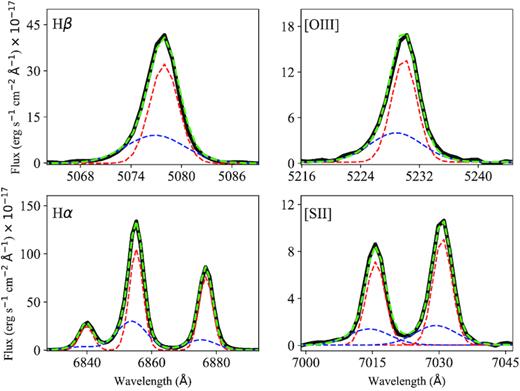
Example of the results from the MCMC spectral modelling for one of the H α-emitting regions in the MaNGA datacubes showing a blue-shifted kinematically distinct component, likely associated with an outflow. The solid, black line is the observed spectrum, the dashed red and dashed blue lines correspond to the narrow and broad kinematic components, respectively, and the dashed green line is the sum of these two components. The values of the parameters for the model represented here correspond to the median of their posterior probability density distributions (see Section 3.4).
4 SAMPLE SELECTION OF OUTFLOW CANDIDATES
Similar to previous works (e.g. Shapiro et al. 2009; Genzel et al. 2011; Soto et al. 2012; Arribas et al. 2014; Gallagher et al. 2018), we consider evidence of outflowing gas only when an extra broad component is clearly identified and it implies velocities significantly larger than those corresponding to the systemic motions in the selected SF regions, as traced by the narrow component. In more detail, we consider the presence of ionized outflows when the following criteria are fulfilled:
Detection of two clear components in emission: We select the cases where both kinematic components have a probability greater than 99.7 per cent of being detected with S/N > 3 integrated in the line, and the contribution of the weakest component to the total line flux is |$\gt 5{{\ \rm per\ cent}}$|.
Presence of radial outflowing gas: We consider that an outflowing component is present when σbroad > 1.4 × σnarrow1 and the broad kinematic component is substantially broader than the one obtained in the single kinematic component fit (σbroad > 1.2 × σ1comp).
Finally, we discard a few cases where the spectra require additional kinematic components, indicative of the presence of type 1 AGN.
We note that as a consequence of applying these criteria the outflows we detect have a minimum FWHMbroad of ∼200 km s−1.
This method for identifying outflows is similar to other ones used in the literature (e.g. Ho et al. 2014; Gallagher et al. 2018; Schreiber et al. 2018). In fact, in the work by Gallagher et al. (2018), where they also used MaNGA data, they found that the broad component is associated with outflowing gas and is characterized by similar FWHMs to the ones we find in our work (>150 km s−1; see Fig. 7 in this paper and fig. 3 in Gallagher et al. 2018).
Using these criteria, we define two samples: one for which we require the two components to be detected at least in the H α line, which contains 105 H α-emitting regions, and a more robust one where the two components have to be detected in all the emission lines included in the spectral fitting, i.e. H α, H β, |${}[\mathrm{N}\,{\small II}]\, \lambda 6583$|, |${}[\mathrm{O}\,{\small III}]\, \lambda 5007$|, |${}[\mathrm{S}\,{\small II}]$| λ6717, 6731, this latter one containing 45 H α-emitting regions. The motivation for using a sample based only on the H α emission is the study of the kinematic properties of the outflow component down to when the contribution is intrinsically weak and/or dust attenuation or geometry (i.e. inclination) hampers the detectability in other lines. We will use the second sample to better characterize the properties of the ionized gas in the outflowing component.
During the analysis of the MaNGA datacubes, we serendipitously detected emission from the supernova candidate 2015co in a galaxy at z ∼ 0.029, whose supernova nature was confirmed and reported in Rodríguez Del Pino et al. (2018).
5 RESULTS AND DISCUSSION
5.1 Outflows detection rate
We start by identifying the outflows that are located in regions away from the central parts of their hosts. Such task is difficult in many cases due to the clumpy nature of the H α emission, limited by the spatial resolution of the instrument, particularly in galaxies with high inclination and at high redshift. Therefore, we only consider as off-nuclear outflows the cases when the broad emission originates in a region that can be spatially isolated from the emission coming from the nuclear parts of the galaxies. Following this method, of the 105 ionized outflows detected in the H α emission, we identify 2 of them in off-nuclear regions at projected distances larger than 1 kpc from the galaxies’ centres. Unfortunately, none of them are detected in other emission lines apart from H α (see Fig. 8). Such low fraction of off-nuclear outflows indicates that most of the outflows tend to originate in the nuclear parts of galaxies. Within the selected sample, we find that a single galaxy is host of three regions showing outflow components (MaNGA 8588-6101), located along a star-forming ring around a central AGN. Although the three regions are located in different regions of the galaxy, the effects from the AGN cannot be discarded; thus, we will not consider them as off-nuclear outflows.
Overall, we detect ionized outflows (at least in H α) in ∼2 per cent of the H α-emitting regions and in |${\sim }7{{\ \rm per\ cent}}$| of the H α-emitting galaxies studied in this work.
We explore the outflows detection rate as the fraction of H α-emitting regions showing outflows for a given local value of the systemic velocity dispersion, σreg, the local H α flux and luminosity (including the contribution from the two components when detected), and a given global value of stellar mass. For this analysis, we show in Fig. 4 the outflows detection rate as a function of the different parameters for the two samples of regions hosting outflows that we have defined in Section 4. We also include the histograms with the distribution of the different parameters for the parent sample of H α-emitting regions.
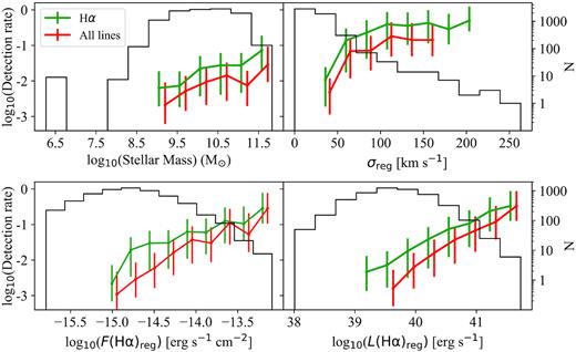
Detection rate of outflows as a function of the stellar mass of the host galaxy and properties of the individual host regions: velocity dispersion of the gas, total H α flux, and total H α luminosity. We represent the detection rate for the sample of outflows detected in H α in green and the sample of outflows detected in all the emission lines in red. The black histograms correspond to the parent sample containing all the individual galaxies (upper left-hand panel) and H α-emitting regions (other three panels).
We find a clear increase in the detection rate of outflows towards higher H α fluxes and luminosities (Spearman’s correlation test probabilities >3σ). In particular, with respect to flux their detection rate increases from |$2.6{{\ \rm per\ cent}}_{-0.3}^{+0.3}$| at fluxes below ∼1.0 × 10⁻¹⁴ erg s−1 cm−2 to |$9.3{{\ \rm per\ cent}}_{-1.5}^{+2.2}$| in regions with fluxes above that value; with respect to luminosity, their detection rate increases from |$1.0{{\ \rm per\ cent}}_{-0.2}^{+0.2}$| at L(H α)≤1040 erg s−1 to |$5.5{{\ \rm per\ cent}}_{-0.6}^{+0.7}$| for higher luminosities. The increase towards higher gas velocity dispersions and stellar masses is less pronounced but still significant (Spearman’s correlation test probabilities >2σ). With respect to gas velocity dispersion, there seems to be a flattening in the detection rate of outflows above σreg >100 km s−1, whereas regarding mass, their detection rate increases from |$1.0{{\ \rm per\ cent}}_{-0.2}^{+0.3}$| at ≤1010 M⊙, to |${\sim }2.9{{\ \rm per\ cent}}_{-0.3}^{+0.3}$| for higher masses. We detect outflows in regions with H α fluxes down to ∼1.0 × 10⁻¹⁵ erg s−1 cm−2, H α luminosities as low as ∼1.1 × 1039 erg s−1 and in host galaxies with stellar masses above ∼1.2 × 10⁹ M⊙.
It is important to note here that we detect ionized outflows at low H α luminosities, corresponding to SFRs down to ∼0.01 M⊙ yr−1 (see Fig. 9), a regime that has only been explored using stacking of spectra from thousands of galaxies (Cicone, Maiolino & Marconi 2016). Therefore, with our analysis we are able to probe ionized outflows down to low SFRs for individual objects, extending the ranges explored by previous works (e.g. Rupke, Veilleux & Sanders 2005; Arribas et al. 2014; Heckman & Borthakur 2016).
Although the detection rate of ionized outflows is low, we have to bear in mind that non-detections do not imply their absence. The detectability of outflows might depend on different factors such as the extinction associated with the outflowing component (as we explore later in this work), the amount of gas in the surroundings, and the efficiency at which the energy is injected into it. Another factor that has been found to influence the detectability of outflows, at least in the neutral phase of the gas, is the inclination of the galaxy (Heckman et al. 2000). To test this dependence in our sample, we estimate the inclinations of the MaNGA DR2 galaxies in the same way as described in Chen et al. (2010): using the axial ratio, b/a, and the r-band absolute magnitude, Mr, of the galaxies (which are taken from the MPA/JHU Value Added Catalogue2) in combination with table 8 from Padilla & Strauss (2008). In the same way as they do, we only consider the inclinations for disc galaxies, which are selected by requiring the parameter fracDeV to be <0.8 (fracDeV quantifies the profile type based on the SDSS best linear combination of an exponential and de Vaucouleurs models). Comparing the inclinations of galaxies in the sample with detected outflows with those in the parent sample, a Kolmogorov–Smirnov test gives a p-value ∼ 0.21, indicating that we cannot reject the hypothesis that the two distributions are the same. The median inclination of galaxies with detected outflows is i ∼ 50°, similar to that of the parent sample of galaxies with H α emission, i ∼ 55°. These two values are also close to the median inclination of the initial sample of 2672 MaNGA DR2 galaxies considered in this study (see Section 2), which is also i ∼ 55°. Thus, we do not find that galaxies hosting ionized outflows have higher inclinations than the rest of the galaxies in our sample. However, we have to bear in mind that due to the generally low incidence of outflows detected any trend with inclinations could be blurred out. On top of that, although the MaNGA sample was not selected based on inclination (Wake et al. 2017), the relatively high inclination of the MaNGA DR2 galaxies (i ∼ 55°) could also hamper the study of inclination effects.
Finally, we explore whether the decline in the outflows detection fraction at low H α fluxes is due only to selection effects (i.e. higher difficulty in detecting two components in fainter lines). We note that trying to establish whether the lack of detections is due to a low observed flux or to a low intrinsic luminosity is difficult because these two quantities are intrinsically correlated. To evaluate the presence of selection effects, we study the probability (obtained from the MCMC modelling) of detecting two emission line components as a function of H α flux and luminosity. This is illustrated in Fig. 5, where we have distributed all the individual H α-emitting regions in different bins of H α flux and luminosity (including the contribution from the two components when detected) and estimated the average probability of detecting two emission line components in H α with S/N > 3. As seen in the plot, the probability increases as a function of the observed flux, indicating selection effects, but also as a function of the intrinsic luminosity, implying that the detectability of outflows is also linked to the intrinsic properties of the host regions. Therefore, the observed decrease in the detection rate of outflows for lower H α fluxes is not only due to selection effects but also to intrinsic lower luminosities.
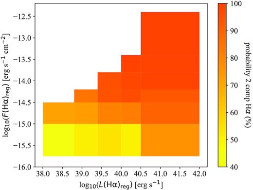
Sample of all the individual H α-emitting regions studied in this work distributed in different bins of total H α flux and luminosity (including the contribution from the two components when detected). The bins are colour coded according to the average probability of detecting two emission line components in H α, with S/N > 3. The bins are chosen to include at least 10 H α-emitting regions therefore covering different parameter ranges (shapes).
5.2 Identifying the ionizing source in the host regions
There is a wide variety of physical mechanisms that can give rise to ionized outflows, such as AGN activity, supernova explosions, stellar winds, and shocks. The differences between the various mechanisms can be primarily quantified using two factors: the kinetic energy injected into the gas and the level of ionization of the gas. The former one can be traced by the kinematics associated with the outflowing component, whereas the latter one can be constrained by mean of standard BPT diagnostic diagrams, (Baldwin, Phillips & Terlevich 1981). In this section, we are interested in characterizing the ionization in the regions hosting outflows, i.e. the systemic (or narrow) kinematic component; therefore, whenever the broad kinematic component is only detected in H α, for the other lines we adopt as systemic value the fluxes measured in the single-component fit.
In the top panels of Fig. 6, we show two versions of the BPT diagram for our sample of regions hosting ionized outflows. On the one hand, the BPT-N diagram (left-hand panel) separates the sources in four different populations using a set of different empirical lines: the dashed line that is used to isolate star-forming regions is the one proposed by Kewley et al. (2001), whereas the dotted line that separates AGN and low-ionization emission regions (LIERs) is taken from Kauffmann et al. (2003b). The area in between these two lines is populated by the so-called ‘intermediate’ population. Finally, the solid line is aimed at separating AGN from LIERs, as suggested by Cid Fernandes et al. (2010). The ‘intermediate’ population corresponds to regions where the level of ionization cannot be explained by either star formation or AGN activity alone (Cid Fernandes et al. 2010) therefore its location in the BPT diagram. First introduced as low-ionization nuclear emission regions (LINERs) by Heckman (1980) because they were associated with nuclear emission, LIERs (Monreal-Ibero, Arribas & Colina 2006; Belfiore et al. 2016) are regions, which can be extended and located away from the nucleus, hosting low levels of ionization that can be produced by low-luminosity AGN, fast shocks, starburst-driven winds, or diffuse ionized plasma (Armus, Heckman & Miley 1990; Dopita & Sutherland 1995; Collins & Rand 2001). On the other hand, the BPT-S diagram (right-hand panel) separates the sources in three types SF, AGN, and LIERs using the lines suggested by Kewley et al. (2001) and Kewley et al. (2006).
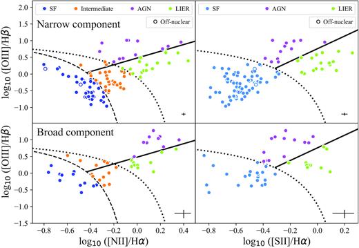
BPT diagnostic diagrams for the narrow (top) and broad components (bottom) in the regions where ionized outflows are detected at least in the H α line. The upper panels contain all 105 the regions hosting outflows (detected in the H α line), whereas the bottom panels contain only the 45 regions where outflows are detected in all the emission lines (see Section 4). The line fluxes used for the upper plots correspond to the systemic (narrow) component or, in the case that the outflow is not detected in all the lines, to the values obtained in the single component fit. The different lines shown in both figures are the empirical separations between ionizing sources of different types, as described in the legend (see Section 5.2 for more details). Typical (mean) error values are shown in the bottom left-hand corner of the panels.
Following these classifications, we find ionized outflows associated with all possible types of ionization, indicating the variety of conditions in which outflows can originate. Based on the results from the two BPT diagnostic diagrams, ionization from star formation is found in 39 per cent of the galaxies using the BPT-N diagram and in 71 per cent of the galaxies using the BPT-S one. The fractions of sources with ionization coming from AGN and LIERs are |${\sim }11{{\ \rm per\ cent}}$| and |${\sim }17{{\ \rm per\ cent}}$|, respectively, being similar in both diagrams. From all the sources classified as ‘intermediate’ in the BPT-N diagram, only one is not classified as star-forming in the BPT-S, corresponding to an AGN located close to the dividing line of the SF population. The two off-nuclear regions hosting outflows identified in this work are classified as star forming in both diagrams.
To complement the analysis presented in the previous section, we evaluate now the detection rate of outflows as a function of the BPT class. We have classified all the regions in the parent sample where all the relevant emission lines are detected with an S/N > 5 (|$\gt 98{{\ \rm per\ cent}}$| of the regions) using both BPT diagnostic diagrams. For this analysis, when two components are clearly detected (Section 4) we adopt the S/N in the narrow kinematic component. The detection rates are presented in Table 1. Our results show that the highest detection rates are associated with regions characterized by AGN and LIER emission, whereas for star-forming regions, which are the largest number in the sample, the detection rates are much lower.
| BPT N ii | BPT S ii | |
|---|---|---|
| AGN | 41.2% | 18.2% |
| LIER | 39.0% | 33.8% |
| Star-forming | 1.0 & | 1.4% |
| Intermediate | 9.4% | – |
| BPT N ii | BPT S ii | |
|---|---|---|
| AGN | 41.2% | 18.2% |
| LIER | 39.0% | 33.8% |
| Star-forming | 1.0 & | 1.4% |
| Intermediate | 9.4% | – |
| BPT N ii | BPT S ii | |
|---|---|---|
| AGN | 41.2% | 18.2% |
| LIER | 39.0% | 33.8% |
| Star-forming | 1.0 & | 1.4% |
| Intermediate | 9.4% | – |
| BPT N ii | BPT S ii | |
|---|---|---|
| AGN | 41.2% | 18.2% |
| LIER | 39.0% | 33.8% |
| Star-forming | 1.0 & | 1.4% |
| Intermediate | 9.4% | – |
Although both BPT diagrams provide relevant information about the ionization mechanisms in our sources, given that both diagrams select almost the same sources as AGN (only one differing object) and LIERs (two differing objects), throughout the paper we will use the BPT-N diagram because it allows a separate study of the SF and ‘intermediate’ populations.
5.3 Outflow properties
5.3.1 Kinematics of the ionized gas
Once we have classified all the regions hosting ionized outflows, we explore the kinematic differences between the outflows originated in them. In Fig. 7, we show the FWHM of the broad kinematic component, FWHMbroad, as a function of the total H α luminosity, obtained as the sum of the H α fluxes in the narrow and broad kinematic components, for the different populations identified in the BPT diagrams. The large scatter indicates that the outflowing gas can have a wide range of velocity dispersions (i.e. FWHM), ranging from ∼200 up to ∼2500 km s−1 in the extreme cases. Apart from this scatter, there are differences in the FWHMbroad for outflows associated with different types of ionization. On average, the regions with SF ionization have outflows with the lowest FWHMbroad, with a median of ∼350 (390) km s−1 in the BPT-N (BPT-S) classification, although these regions can also host outflows with extreme kinematics (≥1000 km s−1). The median FWHMbroad associated with outflows increases progressively for regions classified as ‘intermediate’, (∼450 km s−1), and those classified as AGN (∼550 km s−1) and LIERs (∼900 km s−1), which show similar distributions in both BPT diagrams. These results indicate that there is a clear distinction between the kinematics of outflows originated in regions ionized by different mechanisms, although the ranges of H α luminosities spanned are very similar. We find no significant correlations (Spearman’s correlation tests yield probabilities less than 2σ) between H α luminosity and FWHMbroad for any of the populations identified in the figures. As examples, in Fig. 8 we show the spectral fit to the ionized outflows with FWHMbroad > 1000 km s−1.
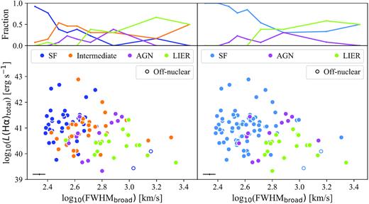
Bottom panels: comparison of the total H α luminosity and the kinematics associated with the ionized outflows detected in the H α, as traced by FWHMbroad. The colours indicate the type of source that is ionizing the gas in the host region, as found in the two BPT diagnostic diagrams shown in Fig. 6. Typical (mean) error values are shown in the bottom corner of the two panels. Top panels: Distributions of FWHMbroad values for the different types of sources.
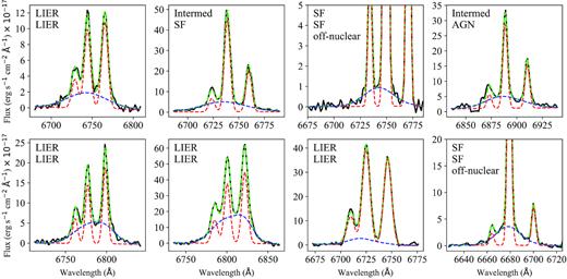
Spectral fit to the outflows with the highest FWHMbroad in our sample. In each panel, we also include the BPT classification based on the BPT-N (top) and BPT-S (bottom) diagnostic diagrams. We also highlight the two cases of off-nuclear outflows. As in Fig. 3, the solid, black line is the observed spectrum, the dashed red and dashed blue lines correspond to the narrow and broad kinematic components, respectively, and the dashed green line is the sum of these two components. The values of the parameters for the model represented here correspond to the median of their posterior probability density distributions (see Section 3.4).
In their study of neutral outflows in a sample of 78 starburst galaxies, Rupke et al. (2005) also found that outflows in LIERs tend to have higher FWHMs than those associated with H ii galaxies, 373 versus 253 km s−1 (median values after converting from their Doppler parameter b). However, the FWHMbroad we measure in the ionized outflows is significantly larger than the ones estimated by Rupke et al. (2005) for the neutral gas phase, |${\sim }110{{\ \rm per\ cent}}$| and |${\sim }50{{\ \rm per\ cent}}$| for LIERs and SF galaxies, respectively, a difference that they reported to be |${\sim }70{{\ \rm per\ cent}}$|.
Interestingly, the outflows in the two off-nuclear, star-forming regions, have FWHMbroad ≥ 1000 km s−1, with H α luminosities 1.86 × 1039 and 2.74 × 1040 erg s−1. Such high kinematics in off-nuclear regions are very unusual, with only a few similar cases been reported in the literature (e.g. Castaneda, Vilchez & Copetti 1990; Gonzalez-Delgado et al. 1994). These events are thought to be associated with a superbubble in the blow-out phase, produced by a large number of massive stars and/or supernovae (Roy et al. 1992). A detailed study exploring the characteristics of these two sources and their possible origin will be presented in a separate paper (Rodriguez Del Pino et al., in preparation).
We extend the study of the kinematic properties of the outflowing gas in Fig. 9, where we show the values of FWHMbroad, ΔV, and Vmax as a function of L(H α), ΣL(H α), and stellar mass of the host galaxy, when available in SDSS DR7, (Kauffmann et al. 2003a). The values of ΣL(H α) are estimated using the areas of the H α-emitting regions defined in Section 3.2. Given that the sizes we estimate (>1−6 kpc) are larger than those typical of star-forming regions (20−100 pc; Miralles-Caballero et al. 2012), the values of ΣL(H α) estimated here should be considered lower limits. The parameter Vmax = |ΔV| + FWHMbroad/2 corresponds to the maximum velocity of the ionized gas, with ΔV being the velocity difference in km s−1 between the narrow and broad kinematic components. The median values of these parameters for the different populations in the BPT-N diagram can be found in Table 2. The data presented in Fig. 9 show that in most of the cases the broad components are blueshifted (negative ΔV) with respect to the systemic emission, providing clear evidence that they are outflows rather than just turbulence. The redshifted component is generally obscured by the host galaxy.
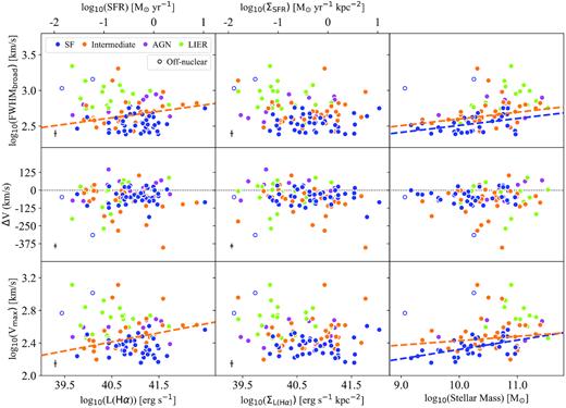
Kinematic properties of the ionized gas as a function of L(H α), ΣL(H α), and stellar mass of the host galaxy for the sources classified according to the BPT-N diagram, using the same colour code as in Fig. 6. In the top axis, we show the corresponding SFR and ΣSFR values that apply for the SF population only. The empty symbols correspond to off-nuclear regions. We represent FWHMbroad, the difference in velocity between narrow and broad kinematic components, ΔV, and the maximum velocity of the ionized gas in the outflow, Vmax, estimated as Vmax = |ΔV| + FWHMbroad/2. The dotted lines at ΔV = 0 in the middle panels are used to separate blueshifted (ΔV < 0) and redshifted outflows (ΔV > 0). When statistically significant correlations between the different parameters are found for a given population, we show them as thick, dashed lines with the colour corresponding to that population. As shown in the plots, we find correlations for the star-forming (blue) and ‘intermediate’ (orange) populations. Typical (mean) error values are shown in the bottom corner of the panels.
Summary of the properties of outflows and host regions for the different ionizing sources identified using the BPT-N diagram. We show the median values and MAD of each parameter in each case.
| SF | Intermediate | LIER | AGN | All sources | ||
|---|---|---|---|---|---|---|
| FWHMbroad (km s−1) | 346 (76) | 452 (75) | 896 (238) | 550 (135) | – | |
| Vmax (km s−1) | 225 (43) | 295 (67) | 497 (104) | 346 (90) | – | |
| F(H α)broad/F(H α)narrow | 0.20 (0.12) | 0.22 (0.15) | 0.45 (0.33) | 0.49 (0.26) | – | |
| AV | Narrow | 1.7 (0.4) | 2.1 (0.4) | 0.8 (0.3) | 1.2 (0.2) | 1.5 (0.5) |
| Broad | 1.7 (1.0) | 2.1 (1.0) | 1.8 (0.7) | 2.4 (0.8) | 1.9 (1.1) | |
| Ne (cm−3) | Narrow | 126 (77) | 248 (81) | 267 (28) | 269 (140) | 222 (122) |
| Broad | 302 (123) | 281 (150) | 706 (264) | 227 (54) | 281 (144) |
As shown in the bottom panels of this figure, outflows in LIERs, with a median value of ∼500 km s−1, have generally associated the largest maximum velocities. In the case of outflows originated in star-forming regions, Vmax is generally below 500 km s−1 (log10(Vmax) ∼ 2.7), with a median value of ∼220 km s−1. However, in some cases they reach values above 1000 km s−1, as it is the case of the off-nuclear regions mentioned above. Such differences with the type of ionization might be associated with low- and high-velocity shocks originated as the gas expands through the interstellar medium (ISM; Rupke et al. 2005; Ho et al. 2014). In fact, as we show in Section 5.3.2, in a significant fraction of the outflows there is evidence for ionization by shocks. The higher velocity of the gas in AGN than in SF outflows has been widely observed (Arribas et al. 2014, and references therein) and is also found in the recent study of outflows in galaxies at redshifts 0.6−2.7 by Schreiber et al. (2018). Contrary to what is found in this latter work, we do not find a correlation between the Vmax and stellar mass for AGN sources, although the low number of AGN with detected outflows (12) prevents us from placing strong constraints.
In the top axis of Fig. 9, we also show the SFR and SFR density, ΣSFR, that applies only for the outflows originated in star-forming regions. We estimate total SFRs following Kennicutt, Tamblyn & Congdon (1994) and using the H α fluxes from the narrow and broad kinematic components. We apply a dust attenuation correction using the reddening curve from Calzetti et al. (2000) and a colour excess E(B − V) given by the Balmer decrement (Domínguez et al. 2013). In this calculation, a value of H α/H β = 2.86 is assumed, which corresponds to a temperature T = 104 K and an electron density Ne = 102 cm−3 for Case B recombination, typical values for star-forming regions. Whenever the outflow is only detected in the H α line, the H β flux used to correct for dust attenuation in the broad component is taken from the single-component fit to the spectra. Again, given the limited spatial resolution of our data, the values of ΣSFR estimated here should be considered lower limits.
We explore now the existence of correlations between the kinematics, star formation properties, and stellar mass of the outflows originated in SF regions. To do that we use a Spearman’s correlation test to study the distribution of the different parameters, not including the two outliers with Vmax > 500 km s−1 to reduce the scatter. From this search, we find a significant strong correlation (p-value < 0.1) of stellar mass with respect to Vmax and a slightly weaker correlation (p-value < 0.3) with respect to FWHMbroad. We show these relations in the top and bottom right-hand panels of Fig. 9 as the dashed, blue lines. This finding indicates that the kinematics of ionized outflows, traced by FWHMbroad and Vmax, increases slightly towards larger stellar masses of the host galaxies, with log−log slopes of ∼0.39 and ∼0.52, respectively. We find a large scatter as a function of SFR and ΣSFR but without any significant trend.
The lack of correlations between outflow kinematics and star formation properties is in contrast with the findings of positive correlations in other works such as the one on local Ultra Luminous Infrared Galaxies (U/LIRGs) by Arribas et al. (2014). However, such differences might be due to the lower regime of SFR probed in this work, barely reaching log10(SFR) > 1 M⊙ yr−1. In fact, our findings agree with the flattening of the relation between outflow velocity and SFR below log10(SFR) ∼ 1 M⊙ yr−1 reported in the SDSS stacking analysis of Cicone et al. (2016). Considering also neutral outflows, the weak correlation we find between Vmax and SFR is also in relative agreement with the large scatter and little correlation found by Rupke et al. (2005) in their study of neutral outflows in local starburst galaxies with SFRs ∼ 50−200 M⊙ yr−1. In fact, they only find a relation when the dwarf galaxies from Schwartz & Martin (2004), whose SFRs are much lower (≤0.1 M⊙ yr−1), are also included. However, such weak correlations are in contrast with those reported by Heckman & Borthakur (2016) for extreme neutral outflows, where a clear correlation is found. Relations between outflow kinematics and stellar mass are more commonly found, both in ionized (Cicone et al. 2016) and in neutral outflows (Heckman & Borthakur 2016).
Considering also other type of sources, we also find relations for the ‘intermediate’ population (also removing the objects with Vmax > 500 km s−1) between the kinematics, (Vmax and FWHMbroad), and both L(H α) and stellar mass. The existence of these correlations as a function of stellar mass is somehow expected because part of the ionizing radiation of these objects must come from star formation, which already correlates with stellar mass. However, the correlations with respect to L(H α), which is not significant for pure, star-forming regions, indicate that additional sources of ionization in these objects might itself correlate with L(H α). LIERs and AGN correspond to more massive systems (on average), but the range in stellar mass (and the limited number of points) is not enough to define a clear correlation.
5.3.2 Ionization by shocks
Many different works on galactic outflows have invoked the presence of shocks in order to reproduce the type of ionization and kinematics observed in the ionized gas (i.e. Monreal-Ibero et al. 2006, 2010; Rich et al. 2010; Westmoquette, Smith & Gallagher 2011; Ho et al. 2014; Wood et al. 2015; Lopez-Coba et al. 2017). These shocks are produced when bubbles of hot gas, originated from supernovae explosions and stellar winds, propagate through the ISM, sweeping up the cool and dense gas. The presence of shock-ionized gas in SF and LIER regions can be identified by the enhancement of the |${}[\mathrm{S}\,{\small II}]$|/H α ratio, which correlates with the velocity of the gas in shock models (Monreal-Ibero et al. 2010; Ho et al. 2014; Lopez-Coba et al. 2017). Since the high |${}[\mathrm{S}\,{\small II}]$|/H α ratios in AGN are not necessarily due to shocks, we do not include them in this analysis.
In Fig. 10, we explore the presence of ionization from shocks in SF, ‘intermediate’, and LIERs regions classified using the BPT-N diagnostic diagram, showing the velocity dispersion of the gas as a function of the |${}[\mathrm{S}\,{\small II}]$|/H α ratio, for the narrow (systemic) and broad kinematic components. In this figure, we only include values for the spectra where the outflow is detected in all emission lines, as explained in Section 4. For reference, we also show in this figure a vertical line at log|$_{10}([\mathrm{S}\,{\small II}]/\mathrm{H}\,\alpha)\,\,\gt -0.5$|, the approximated value at which shock models are able to reproduce the observations (Dopita et al. 2013; Ho et al. 2014). The data presented here show a clear trend between the velocity dispersion of the gas in both kinematic components and |${}[\mathrm{S}\,{\small II}]$|/H α, which can be specially identified in the star-forming population. In general, the |${}[\mathrm{S}\,{\small II}]$|/H α ratio in the broad kinematic component is larger than in the narrow component and in most of the cases above −0.5. This finding indicates that for roughly half of the sample, despite the outflow originating in star-forming regions, the ionization of the outflowing gas could also be due to shocks likely produced when the hot gas propagates through the ISM.
![Velocity dispersion of the narrow and broad kinematic components as a function of the ratio ${}[\mathrm{S}\,{\small II}]$/H α for the sample of outflows in SF regions and LIERs detected in all the emission lines. The vertical line indicates the approximate value at which shock models predict that the gas is ionized by shocks (Dopita et al. 2013). The plot shows that there is a correlation between the velocity dispersion of the broad kinematic component and the ratio ${}[\mathrm{S}\,{\small II}]$/H α. This ratio is also generally higher than in the narrow one. Typical (mean) error values are shown in the bottom left-hand corner of the figure.](https://oup.silverchair-cdn.com/oup/backfile/Content_public/Journal/mnras/486/1/10.1093_mnras_stz816/1/m_stz816fig10.jpeg?Expires=1749168555&Signature=MahO6QJPuojDXZUVbFTkhdsLo4XI7Y9jVjv9hMJLkpjmaL0MPM2r7tsuq~GdTIVnch92TMD7S1smH32Fc2LtNwIfKeOVxCfZ-ppsJ8w4YKAt8jCiiNm3N2SZowe5KAjR5iKtfpKHxVYNKdg3sY430ZA~WQuZSCsvjotHBkVNT-AUiIllY5xssXrdPgO-d5spFPlFhN8JPq0dCfZpikK~q5Ro4MokRSMt8INYntNsxJ39R61XB3~Dwuq15xIAvMCJLzfK1MmyAhSCIMX151AriV-F-jeG8079D68OZtaWGyDOLFknfLLRx~m5iWoSU468BNOCZYy765uOUpUP-xEKQg__&Key-Pair-Id=APKAIE5G5CRDK6RD3PGA)
Velocity dispersion of the narrow and broad kinematic components as a function of the ratio |${}[\mathrm{S}\,{\small II}]$|/H α for the sample of outflows in SF regions and LIERs detected in all the emission lines. The vertical line indicates the approximate value at which shock models predict that the gas is ionized by shocks (Dopita et al. 2013). The plot shows that there is a correlation between the velocity dispersion of the broad kinematic component and the ratio |${}[\mathrm{S}\,{\small II}]$|/H α. This ratio is also generally higher than in the narrow one. Typical (mean) error values are shown in the bottom left-hand corner of the figure.
5.3.3 Extinction
The study of the effects of dust extinction provides relevant information about the material that is being entrained and processed by the outflow as well has the effect that it might have on the observability of the spectral signature of ionized outflows in our spectra. As shown in Section 4, more than half of the outflows detected in the H α line were not detected in other lines such as H β, |${}[\mathrm{O}\,{\small III}]\, \lambda 5007$| and |${}[\mathrm{S}\,{\small II}]$| λλ6717, 6731. This lack of detections could be a consequence of the lower signal to noise in these emission lines, partially due to the effects of dust extinction. To explore these effects, we estimate the extinction associated with the systemic (narrow) and outflowing (broad) gas components, AV,broad and AV,narrow, respectively, following the same procedure explained in Section 5.3.1. We compare the two extinction values in Fig. 11, using the values corresponding to the spectra classified using the BPT-N diagram (Section 5.2) where the broad kinematic component is detected in the H α and H β lines (54 objects). In Table 2, we also show the median values for all the sources and for the different populations.

Comparison of the extinction, AV, for the narrow and broad kinematic components for the sample of outflows detected in the H α and H β lines (54 objects). The solid line is the one-to-one relation. Typical (mean) error values are shown in the bottom right-hand corner of the figure.
The scatter in the values of extinction for both components is quite large, with some values basically consistent with no dust and others reaching values up to 4−5 magnitudes in AV. Considering all the sources, the extinction in the broad component is slightly higher (1.5 and 1.9 for narrow and broad, respectively); however, this difference disappears if only outflows in SF or ‘intermediate’ regions are considered. For AGN and LIERS, although the numbers are low, there seems to be a trend to have higher extinction in the broad component than in the narrow one, a result similar to what is found in type 2 QSOs (Villar Martín et al. 2014). Despite the fact that the differences in AV between the two components are not significant, the effects from extinction can be quite severe, specially in an outflowing component intrinsically broad and with a generally low contribution to the total line flux. Therefore, such high extinction values could contribute to the lack of detections in other spectral lines apart from H α in a significant fraction of the spectra, specially at shorter wavelengths where the effects of dust attenuation are more important.
5.3.4 Density of the gas
An important parameter that characterizes the properties of the systemic and outflowing components is the electron density of the ionized gas associated with them. The electron density can be estimated using the temperature of the ionized gas and the ratio between the fluxes from the |${}[\mathrm{S}\,{\small II}]$| λλ6717, 6731 emission lines (Osterbrock 1989). Assuming a typical temperature for the ionized gas of T = 104 K and following the expressions derived by Sanders et al. (2016), we calculate the electron densities of the two kinematic gas components for the 45 objects where outflows are detected in all the emission lines. The individual values are shown in Fig. 12 and the mean values presented in Table 2. Despite the relatively large uncertainties of the individual values derived using this method (e.g. Genzel et al. 2011; Villar Martín et al. 2014; Perna et al. 2017), we can extract some conclusions. The gas in the outflow tends to be, on average, more dense than the one associated with the narrow component. In particular, in the star-forming regions the median values are 126 cm−3 (Median Absolute Deviation (MAD) = 77) and 302 cm−3 (MAD = 131) for the narrow and broad components, respectively.
![Comparison of the electron densities, ne, estimated using the ${}[\mathrm{S}\,{\small II}]$ λ6717, 6731 lines, for the narrow and broad components. Typical (mean) error values are shown in the bottom right-hand corner of the figure.](https://oup.silverchair-cdn.com/oup/backfile/Content_public/Journal/mnras/486/1/10.1093_mnras_stz816/1/m_stz816fig12.jpeg?Expires=1749168555&Signature=bfbyGgnP9orhfN8-JCWk4Zyuj7E5HkGdpfjcNZgrwlVncrLFN-HB036uk5U6LOZFUqTgGIW0k3a1KoXANcXQG8kCclKl46YdDGwC3tAkyjKryXN3uCuiJKNeqFUT~t88mAGPIqp50vE6nsOLdmbJMQzKcYsfn1aKB9uwINsG9GCgqdKc9WNXVIhTmfX1PYkhzVTNLGXZVixrUsZ1VQfUGpDcaTtY-TVUpVNfTjb3VaoKO56s8FCrGorTk2OQikBm~M3d~UBuLz62oZMh~MFCsN4eFVb7J4llHLEt39YzKIItUfNOReDLvGGEDnVvsr1s7GcTKBtmFyuNekWH4azMsQ__&Key-Pair-Id=APKAIE5G5CRDK6RD3PGA)
Comparison of the electron densities, ne, estimated using the |${}[\mathrm{S}\,{\small II}]$| λ6717, 6731 lines, for the narrow and broad components. Typical (mean) error values are shown in the bottom right-hand corner of the figure.
This finding of overall higher densities in the outflowing components is in agreement, within the uncertainties, with what is found in other works (Arribas et al. 2014; Villar Martín et al. 2014). In summary, the large scatter observed in Fig. 12 demonstrates the wide range of densities that the ionized gas can have. However, the fact that the gas tends to be more dense in the outflowing component might indicate that the pressure is higher, which can also be a consequence of shocks (Ho et al. 2014).
5.4 Global effects of the outflows on the host
5.4.1 Upper estimates of the mass-loading factor
In this section, we explore what is the effect that the ionized outflows studied here can have in the star formation activity of the regions where they are detected. The standard method to evaluate the impact of outflows is to compare the amount of gas that is being ejected by the outflow, referred to as the outflowing mass rate, |$\dot{M}$|, with the amount of gas that is being converted to stars, given by the SFR. The ratio between these two quantities is known as the mass-loading factor, |$\eta = \dot{M}/SFR$|. To estimate η, we follow equation (4) in Arribas et al. (2014), assuming an outflow extension of 0.7 kpc, which is the typical extension found in the extended studies of Bellocchi et al. (2013). As mentioned in Arribas et al. (2014), this derivation of the mass-loading factor assumes that all the gas moves at maximum velocity and does not account for the intrinsic structure of the outflow, which can lead to differences by factors of 2−3 in the estimations of η. Moreover, its estimation is also subject to the large uncertainties in the values of the electron densities (see Section 5.3.4). Based on these assumptions and uncertainties, our estimates of the mass-loading factor should not be considered at face value but instead as upper limits. Although higher resolution studies can obviously characterize better the outflow structure and geometry and therefore provide more accurate estimates of η, the present MANGA data allow us to constrain whether the outflows we study are expected to have or not a significant impact on their surroundings.
In Fig. 13, we show the values of the mass-loading factor, η, for the sample of outflows in SF and ‘intermediate’ regions detected in all the emission lines studied here, as a function of the SFR. We also include the ‘intermediate’ population in this plot because part of the ionization in these sources must come from star formation. The values of η we obtain are in general quite low, with a median value η ∼ 0.25 considering SF and ‘intermediate’ objects; only a few outflows have values larger than 1. Considering that only a small fraction of the gas will be moving at the maximum velocity, our findings indicate that the outflows studied here lead to little, if any, suppression of star formation. In the figure, we also include the data corresponding to the integrated values obtained for U/LIRGs by Arribas et al. (2014) that, despite covering a higher range of SFRs (partially due to be integrated data), generally have larger mass-loading factors than those measured here. Comparing also with the study of outflows at z = 0.6−2.7 by Schreiber et al. (2018), they find slightly lower values (η ∼ 0.1−0.2) than our median estimate, although the SFRs they probe are significantly higher (log10(SFR) ∼ [−1, 2.5]). This similarity could be an indication that, at least since z = 2.7, the impact of ionized outflows driven by star formation in the star formation activity has not been significant. We note here that the estimation of the mass-loading factor only considers the gas that is in the ionized phase and that this value might vary significantly when the neutral and molecular phases are also accounted for.
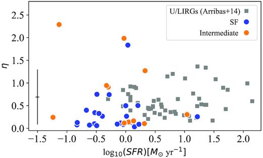
Mass-loading factor, η, as a function of SFR for the sample of ionized outflows in SF regions detected in all the emission lines we explore. For comparison, we also show the values for the integrated properties of U/LIRGs from Arribas et al. (2014). Typical (mean) error values are shown in the bottom left-hand corner of the figure.
Finally, as shown in Table 2, the ratio between the H α fluxes in the narrow and broad components, F(H α)broad/F(H α)narrow, increases significantly from SF and ‘intermediate’ with roughly 20 per cent, to AGN and LIERs, where the broad components encompass around half of the total flux in the narrow ones. This result indicates that outflows in AGN and LIERs entrain relatively larger amounts of ionized gas than those originated in SF and ‘intermediate’ regions.
5.4.2 Gas kinematics and escape velocity
The metal content of galaxies has been proven to be a property that is strongly correlated with the mass of the galaxies, in a way that more massive galaxies have higher metallicities than lower mass ones, following the well-defined mass–metallicity relation (Tremonti et al. 2004; Mannucci et al. 2010). This relation is thought to be held, at least partially, due to the action of outflows regulating the amount of metals formed and kept inside the galaxy (Chisholm et al. 2018). They can regulate the formation of metals by suppressing the star formation and/or drive metal-rich gas out of the galaxies to the IGM (Brooks et al. 2007; Finlator & Dave 2007). In both cases, for a given outflow power, low-mass galaxies are expected to eject more material due to their shallower potential wells. Moreover, the presence of outflows has also been invoked to explain the high metal content of the IGM at high redshift (Aguirre et al. 2001).
The standard method to evaluate whether the gas entrained by an outflow can be expelled from a galaxy is to compare the maximum velocity of the outflowing gas with the escape velocity of the galaxy. This escape velocity can be estimated from the circular velocity of the gas assuming a singular truncated isothermal sphere, as in Heckman et al. (2000). Given that we have not estimated the circular velocity, we follow the method described in Arribas et al. (2014) to estimate escape velocities using the dynamical masses of the galaxies. The dynamical masses are derived from equation (3) in Bellocchi et al. (2013), using the effective radius, the rotational velocity, and the velocity dispersion. In our case, we benefit from the recent release of the MaNGA Value Added Catalogue, which contains a large number of derived parameters for MaNGA DR2 galaxies (Sánchez et al. 2016; Sanchez et al. 2017). From this catalogue,3 we estimate the dynamical masses of the galaxies using the effective radius (Re), the stellar velocity in the central 2.5 arcsec (σcen), and the velocity/dispersion ratio (v/σ) for the stellar populations within 1.5 Re. We note here that v/σ and σcen are estimated using different areas, which could introduce a bias when the velocity dispersion varies significantly within 1.5 Re. However, we expect this difference to be within a factor of ∼2 based on the radial velocity dispersion profiles across different Hubble types (Falcón-Barroso et al. 2017).
In Fig. 14, we show the ratio between Vmax/Vesc as a function of the dynamical mass Mdyn of the galaxies, for our sample of outflows, colour coded following the classification of the BPT-N diagram (Section 5.2). Here, as in Arribas et al. (2014), we have estimated the escape velocity at 3 kpc for an isothermal sphere truncated at 30 kpc.4 Despite all the uncertainties associated with the estimation of Vmax and Vesc, we find a clear trend between their ratio and the dynamical mass of the galaxies. At low dynamical masses the velocity of the ionized gas in the outflow is high enough to overcome the gravitational pull of their hosts, whereas at larger dynamical masses, the increase of the escape velocity reduces the ratio Vmax/Vesc, favouring the withholding of the gas entrained by the outflows. This result is similar to what is found in the study of U/LIRGs by Arribas et al. (2014), although with our sample we extend this trend towards lower dynamical masses. This result agrees nicely with the steep increase of gas-phase metallicity with stellar mass up to 1010.5 M⊙ found by Tremonti et al. (2004). These results indicate that there is a clear connection between the escape velocity and the metallicity of the galaxies, as also reported recently by Barrera-Ballesteros et al. (2018).
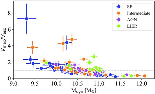
Ratio between the maximum velocity of the gas, Vmax, and the escape velocity, Vesc, as a function of the dynamical mass of the galaxies. The horizontal line corresponds to Vesc/Vmax = 1.
In summary, our results indicate that ejection of gas entrained by ionized outflows to the IGM is more relevant at low dynamical masses, reducing its efficiency towards larger masses. Although the outflow velocities are higher for massive galaxies (see Fig. 9), in general they are not high enough to abandon the potential well of their hosts, retaining the gas, and maintaining their high gas metallicities.
5.4.3 In situ star formation in ionized outflows
Recent works have reported, first in a single system (Maiolino et al. 2017) and more recently in several objects (Gallagher et al. 2018), the detection of star formation taking place inside galactic outflows, this latter work also uses data from MaNGA DR2. This result, predicted by some theoretical models (Ishibashi et al. 2013; Zubovas & King 2014), is of high relevance because it demonstrates that feedback in the form of outflows can enhance star formation, providing a new route for producing stars. Moreover, as explained in Gallagher et al. (2018), the occurrence of star formation inside outflows could help explaining current paradigms such as the early formation of spheroids, the establishment of the relation between black holes and their hosts, and other observed properties.
The identification of outflowing gas ionized by stars does not by itself prove the presence of ionizing starts within the outflow. It could also be possible that the photons from stars located in the disc ionize the outflowing gas. To distinguish between these two scenarios, and following (Maiolino et al. 2017) and Gallagher et al. (2018), here we explore the values of the ionization parameter, which is expected to be significantly lower when the gas is far from the ionizing stars (all the other properties being equal). We do that by comparing the values of the ionizing parameter, U, that describes the degree of ionization of the gas, for both kinematic components. Following Diaz et al. (2000), we calculate this parameter as the ratio between |$[\mathrm{O\,\small III}]\, \lambda 5007$| and the sum of the |$[\mathrm{O\,\small II}]\lambda \lambda 3727,3730$| lines.5 Here, we use only regions hosting outflows ionized by star formation, for which we select the sources whose broad component is located in the SF region of the BPT-N diagram in the bottom panels of Fig. 6. We note that this way of estimating U is subject to differences in the density of the gas (favouring larger values of U for higher densities) and to the effects of dust extinction (favouring higher values of U if the extinction is high). Note, however, that the electron densities for the narrow and broad components in star-forming galaxies are consistent with each other within a factor of ∼1.5 (Table 2) and that we have estimated AV for each component therefore our U estimates account for them. Following Gallagher et al. (2018), we also estimate the parameter R23, defined as the ratio (|$[\mathrm{O\,\small III}]\lambda \lambda 4960,5007$| + |$[\mathrm{O\,\small II}]\lambda 3727$|)/H β, for both components.
The results, presented in Fig. 15, show that the ionizing parameter U (traced by the ratio |$[\mathrm{O\,\small III}]\, \lambda 5007$|/|$[\mathrm{O\,\small II}]\lambda \lambda 3727,3730$|) is quite similar in both kinematic components, with only one case where the ratio Unarrow/Ubroad is larger than ∼10. Given that U decreases with the square of the distance, we can use this result to evaluate whether the star formation ionizing the outflowing gas is coming from the disc of the galaxy or from inside the outflow. To do that, since we do not have accurate estimates of the sizes of the star-forming regions nor the extension of the outflows, we use standard values from the literature: typical sizes of star-forming knots are 20−100 pc (e.g. Miralles-Caballero et al. 2012), whereas the extension of outflows in similar galaxies is ∼0.7 kpc (Bellocchi et al. 2013, median value from table 5). Assuming these sizes, if the stars ionizing the outflowing gas resided in the disc of the galaxies (at a distance typically ∼7 × the size of the region), the ionizing parameter U in the broad component would be a factor ∼50 lower than observed. However, the values shown in Fig. 15 do not suggest such large differences, indicating that our results are consistent with star formation taking place within the ionized outflows, as previously reported by Maiolino et al. (2017) and Gallagher et al. (2018). We note here that this result only holds under the assumption (based on estimates from other works) that the outflowing regions are significantly larger than individual star-forming ones.
![Comparison of the ionizing parameter, U, traced by the ratio $[\mathrm{O\,\small III}]\, \lambda 5007$/$[\mathrm{O\,\small II}]\lambda \lambda 3727,3730$, as a function of the R23 parameter (see text for details) for both kinematic components, similar to fig. 7 in Gallagher et al. (2018). Values take into account individual estimates for AV. Here, we show only the cases where the broad component is ionized by star formation. Since the ionizing parameter is similar in both components, the outflowing gas must be ionized by in situ star formation (see Section 5.4.3 for details).](https://oup.silverchair-cdn.com/oup/backfile/Content_public/Journal/mnras/486/1/10.1093_mnras_stz816/1/m_stz816fig15.jpeg?Expires=1749168555&Signature=3DOeCWfe8vy4zUycavS4XwVaNp1Qoxp5fyqUnIplViDqI0w1pOyxVOg1g8rhcnijfsC6jv90zCyIm~lXbRJcr9sdnP54yXvKcpbWBKxtjUewNQtxxIcN5coJ5O0ohFv0-KVhpNChgWYKXRiGoHOJgmfBPah5VEXww5l4CJefCXk4ayvz-fRxz1pYq771jmuhft5exz1cSaK3NO2VxLUVgTBEpAaoYU5djs3jW71WSbnI7MgE8chaP7LsJkVNgcWx11D9ME21dK5yr8~QH3U-D0sOO7GSrvhEMalp2jR6kSExTk7GWkTPZlTP9pp9J63V6fPDhqjTzi5EhIkQBxdgYg__&Key-Pair-Id=APKAIE5G5CRDK6RD3PGA)
Comparison of the ionizing parameter, U, traced by the ratio |$[\mathrm{O\,\small III}]\, \lambda 5007$|/|$[\mathrm{O\,\small II}]\lambda \lambda 3727,3730$|, as a function of the R23 parameter (see text for details) for both kinematic components, similar to fig. 7 in Gallagher et al. (2018). Values take into account individual estimates for AV. Here, we show only the cases where the broad component is ionized by star formation. Since the ionizing parameter is similar in both components, the outflowing gas must be ionized by in situ star formation (see Section 5.4.3 for details).
Finally, given that we only detect outflows in |${\sim }2{{\ \rm per\ cent}}$| of the H α-emitting regions and that the upper estimates of the mass-loading factors are generally low (η ∼ 0.25; Section 13), our results indicate that any in situ star formation in the galaxies studied here would not have a strong impact in their evolution.
6 SUMMARY AND CONCLUSIONS
In this work, we have presented the results from a systematic search and characterization of ionized outflows in nuclear and off-nuclear H α-emitting regions of more than 2700 nearby galaxies (z ≤ 0.15) from MaNGA DR2. The galaxies have stellar masses in the range ∼109−1012 M⊙ and the SFRs span from ∼0.01 to ∼10 M⊙ yr−1. In total, we have identified and analysed the spectra of ∼5200 H α-emitting regions from ∼1500 individual systems, with a mean of ∼3.5 regions per galaxy, searching for spectral signatures of ionized outflows. Ionized outflows are detected, at least in the H α line, in a total of 105 individual H α-emitting regions, corresponding to 103 individual galaxies. From this sample, in 45 cases the secondary component is also detected in H β, |$[\mathrm{O\,\small III}]\, \lambda 5007$| and |${}[\mathrm{S}\,{\small II}]$| λ6717, 6731. In this work, we extend the study of ionized outflows to regions with SFRs as low as ∼0.01 M⊙ yr−1, a SFR regime lower than those explored by previous works on individual systems.
We have explored the differences in the kinematics and properties of the ionized gas for the systemic and outflowing components in regions classified as star-forming, ‘intermediate’, LIER, and AGN based on the type of ionization, and analysed the feedback effects. The main results we have obtained in our work can be summarized as
We detect ionized outflows in ∼2 per cent of the H α-emitting regions and in ∼7 per cent of the H α-emitting galaxies studied in this work. The detection rate of ionized outflows increases with H α flux and stellar mass of the host galaxies. Considering all the H α-emitting regions identified in this work, their incidence varies from less than |$2{{\ \rm per\ cent}}$| at fluxes below ∼1.0 × 10⁻¹⁴ erg s−1cm−2 to more than |$8{{\ \rm per\ cent}}$| in regions with fluxes above that value. Regarding mass, their incidence increases at ∼1010 M⊙, when they are detected in |${\sim }3{{\ \rm per\ cent}}$| of the cases.
We find only two off-nuclear outflows, located at distances larger than 1 kpc from their galaxies’ centres. These outflows show extreme gas kinematics (Vmax > 500 km s−1 and FWHMbroad > 1000 km s−1), although they are only detected in the H α line. The origin of such remarkable features is still unclear and will be explored in more detail in a separate paper (Rodríguez Del Pino et al., in preparation).
We find significant differences in the gas kinematics of outflows originated in regions with different type of ionization. Regions characterized by LIER emission host the outflows with more extreme kinematics (FWHMbroad ∼ 900 km s−1), followed by those originated in AGN, ‘intermediate’, and SF regions (FWHMbroad ∼ 550 km s−1, ∼450 km s−1, ∼350 km s−1, respectively). A similar result is found for the maximum velocities of the gas, Vmax. These differences might be due to the presence of low- and high-velocity shocks, given the high incidence of outflowing, shock-ionized gas detected in our sample.
Considering only pure, SF regions, we find significant correlations between the kinematics of the outflowing gas and the stellar mass of the host galaxies, implying higher FWHMbroad and Vmax with increasing stellar mass (log−log slopes of ∼0.39 and ∼0.52, respectively). However, no significant correlations are found between gas kinematics and star formation properties SFR and ΣSFR, probably due to the lower SFR regime probed in this study. Moreover, the gas kinematics in ‘intermediate’ regions correlates both with the stellar mass L(H α), probably as a consequence of the additional mechanisms responsible for the ionization of the gas in these sources.
Although the uncertainties in the estimation of the electron densities are relatively large, the gas is generally denser in the outflowing component, pointing towards a shock-related origin of the outflows.
We estimate mass-loading factors, η, generally below 1, with a median value η ∼ 0.25 considering both SF and ‘intermediate’ regions. Therefore, despite all the uncertainties associated with the mass-loading factor estimates, the ionized outflows studied in this work do not suggest a strong impact in the star formation activity in the host regions.
Our analysis shows that only at low masses (M < 1010 M⊙) part of the gas entrained by the outflows is able to escape the gravitational well of the galaxy. At high masses, outflows are probably only able to produce gas fountains that would return the gas to the galaxies. This relation between the fraction of gas that can abandon the galaxy as a function of mass could help explaining the existent correlation between the gas-phase metallicity and the stellar mass of galaxies (Tremonti et al. 2004; Mannucci et al. 2010).
The values of the ionization parameter measured in the systemic and outflowing components in regions hosting outflows ionized by star formation are consistent with in situ star formation, under the assumption (based on estimates from other works) that the outflowing regions are significantly larger than individual star-forming ones. This result implies that at least a fraction of our sample of outflows are compatible with the recently reported finding of star formation taking place inside ionized outflows (Maiolino et al. 2017; Gallagher et al. 2018). However, although the uncertainties are large and we only probe the ionized phase of the outflowing gas, the low mass-loading factors we measure indicate that in situ star formation does not have a significant impact in the galaxies studied here.
ACKNOWLEDGEMENTS
We thank the anonymous referee for comments and suggestions that have contributed to improve the paper. BRP, SA, and LC acknowledge support from the Spanish Ministry of Economy and Competitiveness through grants ESP2015-8964 and ESP2017-83197. JPL acknowledges support from the Spanish Ministry of Economy and Competitiveness through grant AYA2017-85170-R. MVM acknowledges support from the Spanish Ministry of Economy and Competitiveness through the grant AYA2015-64346-C2-2-P. Funding for the SDSS-IV has been provided by the Alfred P. Sloan Foundation, the U.S. Department of Energy Office of Science, and the Participating Institutions. SDSS-IV acknowledges support and resources from the Center for High-Performance Computing at the University of Utah. The SDSS web site is www.sdss.org. This research made use of Astropy, a community-developed core Python package for Astronomy Astropy Collaboration et al. (2018). This project makes use of the MaNGA-Pipe3D dataproducts. We thank the IA-UNAM MaNGA team for creating this catalogue, and the ConaCyt-180125 project for supporting them.
Footnotes
In a few cases where the lines are barely resolved (i.e. the line width is close to that of the line spread function), we ensure that σbroad is also 1.4 × larger than the instrumental broadening, σinst, at the given wavelength. In these cases, we visually inspect the spectra to check that the classification is adequate.
The choice of the truncated value of the sphere at 30 kpc is somewhat arbitrary. However, we note that the values of Vesc change by less than 20 per cent if the truncated value is placed at 100 kpc, introducing no significant changes in our results.
For this analysis, we repeat the same fitting procedure explained in Section 3.4 but including in the fits the |$[\mathrm{O\,\small II}]\lambda \lambda 3727,3730$| lines. In this case, the subtraction of the stellar component is done using the MILES library (Sánchez-Blázquez et al. 2006), whose wavelength coverage is 3525–7500 Å. To select the sample, we apply the same selection criteria as in Section 4 to the |$[\mathrm{O\,\small II}]\lambda \lambda 3727,3730$| lines.
