


Abstract
Magnetars are neutron stars with extremely high surface magnetic fields. They show diverse X-ray pulse profiles in the quiescent state. We perform a systematic Fourier analysis of their soft X-ray pulse profiles. We find that most magnetars have a single-peaked profile and hence have low amplitudes of the second Fourier harmonics (A2). On the other hand, the pulsed fraction (PF) spreads over a wide range. We compared the results with theoretical profiles assuming various surface hotspot asymmetries, viewing geometries, and beaming functions. We found that a single value of the intensity ratio r between two antipodal hotspots is unable to reproduce the observed distribution of A2 and PF for all magnetars. The inferred r is probably anticorrelated with the thermal luminosity, implying that high-luminosity magnetars tend to have two symmetric hotspots. Our results are consistent with theoretical predictions, for which the existence of an evolving toroidal magnetic field breaks the symmetry of the surface temperature.
1 INTRODUCTION
Magnetars are isolated neutron stars (NSs) exhibiting dramatic timing variabilities and are believed to have extraordinarily high surface magnetic fields (see the review by Kaspi & Beloborodov 2017). They have spin periods clustering in the range of P = 2–12 s, large spin-down-inferred dipolar magnetic fields of B = 1012–1016 G, and high surface luminosities of L ≈ 1031–1036erg s−1 in the quiescent state. The most remarkable feature of magnetars is burst in soft gamma-ray/hard X-ray bands. The intense bursting epochs are usually accompanied with outbursts, during which the persistent X-ray luminosity increases dramatically on a short time-scale and then decays slowly for months to years. The mechanisms triggering the outburst remain a puzzle. The energy could be injected from the deep layer of the crust through magnetic dissipation or from the interaction between the currents along the twisted magnetic field lines and the stellar surface (Lyubarsky, Eichler & Thompson 2002; Beloborodov & Thompson 2007; Beloborodov 2009; Pons & Rea 2012). The bombardment of particles from the magnetosphere produces additional hotspots and provides a possible heating source (Beloborodov & Thompson 2007; Beloborodov & Li 2016). Observations show that the hotspot temperature decreases and the corresponding area shrinks during the flux relaxation of the outburst (see e.g. Rea et al. 2013; Coti Zelati et al. 2015; Mong & Ng 2018). The emerging hotspots generally cause extra peaks in the pulse profile, while the strength of the peak decreases as the flux decreases (see e.g. Rodríguez Castillo et al. 2014). The shape of the pulse profile usually evolves back to the pre-outburst state within months to years. Several magnetars, such as 4U 0142 + 61, have no recorded major outburst, although they could have subtle flux variability. Their quiescent fluxes and profiles show moderate variabilities but are relatively stable compared with the change during outbursts (Dib, Kaspi & Gavriil 2007).
The high X-ray luminosity of magnetars is believed to be powered by the decay of the strong B field, although the conversion mechanism is elusive. The magneto-thermal evolution model suggests that magnetic energy is transferred to heat through the dissipation process in the crust. This model explains the systematically high surface temperature of magnetars and unifies the temperature evolution of various NS populations (Kaminker et al. 2006, 2009; Pons, Miralles & Geppert 2009; Perna & Pons 2011; Ho, Glampedakis & Andersson 2012; Viganò et al. 2013; Kaminker et al. 2014). Instead of having a pure dipole B field, magnetars are believed to have complex B-field structures such as a toroidal component (Thompson, Lyutikov & Kulkarni 2002; Pavan et al. 2009; Viganò et al. 2013). These components make the total B field stronger than the observable dipolar term and enhance the decay of the B-field strength. This process increases the heating of the NS surface and extends the cooling time-scale. It also breaks the B-field symmetry, resulting in an asymmetric surface temperature distribution owing to either the suppression of the temperature of one hotspot or the migration of the coldest/hottest part from the magnetic equator/poles (Ng et al. 2012; Viganò et al. 2013). The change in the surface temperature symmetry can be inferred from the quiescent thermal pulse profile. Previous studies revealed highly modulated single-peaked pulse profiles for some magnetars (e.g. Tam et al. 2008; Zhou et al. 2014). It could indicate an asymmetric surface temperature distribution and cannot be explained by two hotspots located at the magnetic poles with similar luminosities (Perna et al. 2013). For a magnetar with a strong initial toroidal field, it is expected that the pulse profile is time-dependent and could be correlated with the B-field strength, the age, or the thermal luminosity. This motivated us to perform a systematic analysis of magnetars thermal pulse profiles. Similar analyses have been applied to several individual magnetars to trace the pulse-profile evolution on various time-scales (e.g. DeDeo, Psaltis & Narayan 2001; Tam et al. 2008; Şaşmaz Muş & Göğüş 2013), but a comprehensive investigation of all currently known magnetars is lacking. We thus parametrize the quiescent soft X-ray pulse profiles of magnetars and investigate their connection to physical parameters.
We introduce the source selection and the basic reduction of the Chandra and XMM–Newton data in Section 2. Then, we describe the pulse-profile analysis method in Section 3. The results for individual sources and the observed distribution of pulse-profile parameters are described in Section 4. We present simulations and discuss the evolution of the surface temperature anisotropy in Section 5. The connection between the observed pulse profiles and the surface intensity distribution is described in Section 6. Finally, we summarize this work in Section 7. We also found that the previously reported timing solutions of CXOU J171405.7 – 381031 are highly variable. We perform a timing analysis on several new data sets to update the |$\dot{P}$| value in Appendix A.
2 SOURCE SELECTION AND X-RAY DATA REDUCTION
We selected the sample from the McGill Online Magnetar Catalog1 (Olausen & Kaspi 2014). There are 23 confirmed magnetars to date. We utilized the data collected with Chandra and XMM–Newton owing to their excellent sensitivity below 2 keV. We checked the outburst history of magnetars from the Magnetar Outburst Online Catalog2 (Coti Zelati et al. 2018). We chose observations that were taken at least half a year after the onset of an outburst (or the first observation available since the outburst if the onset time is unknown) and have a flux that decreased to ∼10 per cent of the peak flux. From a total of 23 magnetars, we analysed 18. We could not obtain pulse profiles for the remaining ones. For example, SGR 0526 – 66 showed a pulsating tail with P ≈ 8 s after a giant flare (Cline et al. 1980). A similar period was marginally determined in two Chandra and one XMM–Newton data sets (Kulkarni et al. 2003; Tiengo et al. 2009). However, no stable pulse profile could be obtained from the data sets. Moreover, we did not detect any significant periodicity in PSR J1622 − 4950, SGR 1627 − 41 and Swift J1834.9 − 0846. Finally, SGR 1833 − 0832 was not detected in either Chandra or XMM–Newton observations before its outburst. Fig. 1 shows the outburst history of all sampled magnetars and the observation epoch of the data sets used in this research.
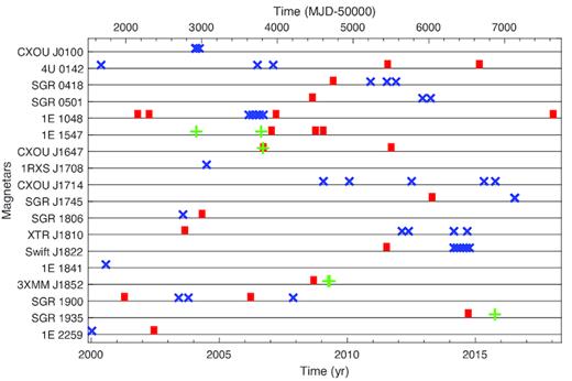
Outburst history of all magnetars and the distribution of data sets used in this analysis. The red squares denote the onset epochs of the outbursts, the blue crosses are the Chandra observation epochs, and the green plusses are the XMM–Newton observation epochs for individual magnetars. Only those data sets used in this analysis are plotted.
To investigate the shape of pulse profiles, observations with high timing resolution are necessary. Therefore, the data taken with the Chandra Advanced CCD Imaging Spectrometer (ACIS) in the continuous-clocking (CC) mode is preferred, because its timing resolution is as high as 2.85 ms. For sources without CC-mode observations, we utilized the 1/8 subarray timed-exposure (TE) mode observations (timing resolution of ∼0.4 s) in order to minimize the contamination from the surroundings. For the remaining sources without Chandra observations in quiescence, we investigated their pulse profiles with XMM–Newton observations. The PN detector has a timing resolution of 74 ms for the full-frame (FF) mode observation, while it is 2.6 s for the MOS detectors. Therefore, we mainly utilized the data obtained with the PN detector. We calculated the background-subtracted pulse profiles for all sampled magnetars. All the observations used in this analysis are summarized in Table 1.
Data sets used in this analysis.
| Name | Instrument/Modea | Data set (ObsID) |
|---|---|---|
| CXOU J010043.1 – 721134 | Chandra/TE | 1881, 4616, 4617, 4618, 4619, 4620 |
| 4U 0142 + 61 | Chandra/CC | 724, 6723, 7659 |
| SGR 0418 + 5729 | Chandra/TE | 13148, 13235, 13236 |
| SGR 0501 + 4516 | Chandra/TE | 14811, 15564 |
| 1E 1048.1 – 5937 | Chandra/CC | 6733, 6734, 6735, 6736, 7347 |
| 1E 1547.0 – 5408 | XMM PN/FF | 0604880101 |
| CXOU J164710.2 – 455216 | XMM PN/FF | 0404340101 |
| 1RXS J170849.0 – 400910 | Chandra/CC | 4605 |
| CXOU J171405.7 – 381031 | Chandra/CC | 10113, 11233, 13749, 16762, 16763 |
| SGR J1745 – 2900b | Chandra/TE | 18731, 18732 |
| SGR 1806 – 20b | Chandra/CC | 4443 |
| XTE J1810 – 197 | Chandra/TE | 13746, 13747, 15870, 15871 |
| Swift J1822.3 – 1606 | Chandra/TE | 14819, 15988, 15989, 15990, 15991, 15992, 15993 |
| 1E 1841 – 045 | Chandra/CC | 730 |
| 3XMM J185246.6 + 003317 | XMM MOS/FF | 0550671301, 0550671801, 0550671901 |
| SGR 1900 + 14 | Chandra/CC | 3863, 3864, 8215 |
| SGR 1935 + 2154 | XMM PN/FF | 0764820201 |
| 1E 2259 + 586 | Chandra/CC | 726 |
Notes. aCC, Chandra ACIS continuous-clocking mode; TE, Chandra ACIS timed-exposure 1/8 subarray mode; FF, XMM–Newton full-frame mode.
bWe extended the high-energy boundary of the pulse profile to 4 keV to boost the signal-to-noise ratio (see text).
We downloaded the Chandra data from the Chandra Data Archive,3 and reprocessed them using the pipeline 'chandra_repro' in the Chandra Interactive Analysis of Observations (ciao) version 4.9 with the calibration data base (caldb) version 4.7.3 (Fruscione et al. 2006). All the photon arrival times were corrected to the barycentre of the Solar system using the task 'axbary' based on the JPL ephemeris DE405. We extracted the source photons from a 4-arcsec-wide box centred on the source for CC mode observations. The fractional encircled flux is energy-dependent, and this selection criterion contains an average of ∼90 per cent of the source flux. The source selection criteria used for the Chandra TE mode and XMM–Newton observations also contain ∼90 per cent of the source flux. The background events were extracted from a box with the same size in a nearby region. For Chandra data taken in the 1/8 subarray TE mode, we extracted the source photons from a 2-arcsec-radius circular aperture centred on the source, and extracted background events from nearby source-free regions.
For XMM–Newton, we downloaded the data from the XMM–Newton Science Archive4 and reduced them using the XMM–Newton Science Analysis Software (sas) version 16.0.0. We reprocessed the PN data with current calibration files using 'epproc'. After the reduction, we corrected the photon arrival time to the barycentre of the Solar system using 'barycen' with the JPL ephemeris DE405. The time intervals with flaring particle background were filtered out. We then extracted the source photons from a circular aperture with a 40-arcsec radius, and the background events from nearby source-free regions. For 3XMM J1852, all the observations were pointed to the nearby pulsar J1852 + 0040, and PN was operated in the small-window mode. As a result, 3XMM J1852 lay outside the PN field of view. We therefore utilized the MOS data. We used 'emproc' to reprocess the data and performed all the necessary corrections to photon events as for the PN data. Then we combined the events collected from both the MOS1 and the MOS2 detector for the timing analysis.
3 ANALYSIS METHOD
Given that we are focusing on the quiescent soft X-ray pulse profile, we chose to analyse the events in the energy range of 0.5–2 keV. SGR 1745 − 2900 and SGR 1806 − 20 are exceptional owing to an insufficient photon count (see Table 1). A precise spin period is needed to investigate the detailed pulse-profile structures, but some new observations are not covered by published ephemerides (see e.g. Dib & Kaspi 2014). Moreover, many magnetars have no long-term ephemerides. We therefore searched the periods in individual data set using the H-test algorithm (de Jager, Raubenheimer & Swanepoel 1989) and obtained their soft X-ray profiles, in which the emission is dominated by the surface thermal emission. For magnetars with multiple observations, we searched their periods individually. We verified that the profile did not change significantly between observations. We then assigned the pulse phase to each photon with respect to a fiducial point, for example the valley of the pulse. We combined all the photon events to create a stacked pulse profile. The pulse profile could have minor variability between observations as a result of noise. However, we checked that there were no significant variabilities (e.g. from single-peaked to double-peaked). We divided the pulse profile into 64 phase bins. We also performed our analysis using 16 and 32 bins, but found that the results were consistent across each choice of binning. We calculated the uncertainty of each phase bin in the folded light curve by assuming a Poisson distribution for the photons. The background folded light curve was created according to the same timing solution and then was subtracted from the source profile. The background-subtracted pulse profiles of sampled magnetars are plotted in Fig. 2.


Soft X-ray profiles (0.5–2 keV) of sampled magnetars and the corresponding strength of Fourier components. The histogram and red curve in the upper panel of each source denote the observed pulse profile and the reconstructed one from the first five Fourier harmonics. The pulse profile of each source is normalized to its mean photon counts. The bin sizes shown here vary between sources and are chosen purely for illustrative purposes. The normalized Fourier power of the first five harmonics is plotted in the lower panel for each source.
We only collected ∼30 X-ray photons in 0.5–2 keV from SGR J1745 − 2900 owing to the heavy absorption (Coti Zelati et al. 2015). We then calculated the H value for different energy bands. For each calculation, we set the low-energy boundary to 0.5 keV and let the high-energy boundary Eh vary from 2 to 7 keV. We found that the H value increases monotonically starting from Eh = 3 keV and reaches a plateau at Eh ≳ 5.5 keV. The pulse profile in 0.5–4 keV results in H = 63, corresponding to a detection significance of 6.5σ (de Jager & Büsching 2010). We therefore calculated the parameters of the pulse profile at ≲ 4 keV. Similarly, the X-ray photons collected from SGR 1806 − 20 below 2 keV are insufficient for a timing analysis. In addition, the pulse profile above 4 keV could be very different from that below 4 keV (Younes, Kouveliotou & Kaspi 2015). We therefore extended the high-energy boundary to 4 keV to increase the X-ray photon numbers.
4 RESULTS
4.1 Distribution of profile parameters
We applied the above analysis techniques to the selected data sets and summarize the PF values and the strengths of the first two Fourier components of sampled magnetar profiles in Table 2. None of the magnetars in our sample shows significant triple-peaked or more complex profiles in quiescence. Therefore, the strengths of A3–A5 are generally negligible, and we do not list them in Table 2. We also give the spin parameters (P and |$\dot{P}$|), spin-down-inferred parameters (B field and characteristic age τc), and the age measurements from the supernova remnants (SNRs) if available. We also list their thermal luminosities in the table (see Appendix B).
Physical properties and derived parameters of the sampled magnetars.
| Name | Pa | |$-\log {\dot{P}}^a$| | B fielda | |$\tau _c^a$| | SNR age | log Lb | A1 | A2 | PFc |
|---|---|---|---|---|---|---|---|---|---|
| [s] | [1014 G] | [kyr] | [kyr] | [erg s−1] | |||||
| CXOU J0100 | 8.02 | 10.72 | 3.9 | 6.8 | – | |$35.4^{+0.4}_{-0.3}$| | 0.40 ± 0.04 | 0.30 ± 0.04 | 0.20 ± 0.01 |
| 4U 0142 | 8.69 | 11.69 | 1.3 | 68 | – | |$35.5^{+0.2}_{-0.3}$| | 0.45 ± 0.02 | 0.42 ± 0.02 | 0.047 ± 0.001 |
| SGR 0418 | 9.08 | 14.40 | 0.061 | 36000 | – | |$31.0_{-0.8}^{+0.6}$| | 0.64 ± 0.09 | 0.09 ± 0.05 | 0.37 ± 0.03 |
| SGR 0501 | 5.76 | 11.22 | 1.9 | 16 | 4–7 | |$33.5_{-1.1}^{+0.7}$| | 0.38 ± 0.03 | 0.28 ± 0.03 | 0.28 ± 0.01 |
| 1E 1048 | 6.46 | 10.65 | 3.9 | 4.5 | – | 34.8 ± 0.2 | 0.79 ± 0.01 | 0.152 ± 0.006 | 0.584 ± 0.004 |
| 1E 1547 | 2.07 | 10.32 | 3.2 | 0.69 | – | |$33.1_{-0.8}^{+0.4}$| | 0.73 ± 0.06 | 0.07 ± 0.03 | 0.205 ± 0.009 |
| CXOU J1647 | 10.61 | 12.01 | 1.0 | 173 | – | |$33.8_{-0.7}^{+0.4}$| | 0.63 ± 0.08 | 0.14 ± 0.05 | 0.47 ± 0.04 |
| 1RXS J1708 | 11.01 | 10.71 | 4.7 | 9.0 | – | 34.7 ± 0.2 | 0.69 ± 0.02 | 0.21 ± 0.01 | 0.294 ± 0.004 |
| CXOU J1714 | 3.83 | 10.19 | 5.0 | 0.95 | |$0.65^{+2.50}_{-0.30}$| | |$34.9^{+0.7}_{-1.1}$| | 0.63 ± 0.07 | 0.13 ± 0.04 | 0.31 ± 0.02 |
| SGR J1745 | 3.76 | 10.86 | 2.3 | 4.3 | – | |$34.2_{-0.3}^{+0.2}$| | 0.62 ± 0.07 | 0.07 ± 0.04 | 0.26 ± 0.03 |
| SGR 1806 | 7.55 | 9.31 | 20 | 0.24 | – | |$35.3_{-0.3}^{+0.2}$| | 0.41 ± 0.08 | 0.24 ± 0.07 | 0.10 ± 0.02 |
| XTE J1810 | 5.54 | 11.11 | 2.1 | 11 | – | |$34.6_{-0.3}^{+0.2}$| | 0.74 ± 0.06 | 0.08 ± 0.03 | 0.212 ± 0.009 |
| Swift J1822 | 8.44 | 13.68 | 0.14 | 6300 | – | |$33.0_{-0.9}^{+0.6}$| | 0.69 ± 0.06 | 0.14 ± 0.03 | 0.33 ± 0.02 |
| 1E 1841 | 11.79 | 10.39 | 7.0 | 4.6 | 0.5–1 | |$35.3_{-0.5}^{+0.4}$| | 0.50 ± 0.09 | 0.19 ± 0.07 | 0.11 ± 0.02 |
| 3XMM J1852 | 11.56 | >12.85 | <0.41 | >1300 | – | |$33.7_{-0.6}^{+0.4}$| | 0.67 ± 0.07 | 0.09 ± 0.04 | 0.52 ± 0.04 |
| SGR 1900 | 5.20 | 10.04 | 7.0 | 0.9 | – | |$35.0_{-0.3}^{+0.2}$| | 0.50 ± 0.08 | 0.15 ± 0.06 | 0.11 ± 0.01 |
| SGR 1935 | 3.25 | 10.87 | 2.2 | 3.6 | – | |$34.2_{-0.6}^{+0.4}$| | 0.5 ± 0.01 | 0.13 ± 0.06 | 0.10 ± 0.02 |
| 1E 2259 | 6.98 | 12.32 | 0.59 | 230 | 14 ± 0.02 | 34.8 ± 0.2 | 0.21 ± 0.01 | 0.53 ± 0.02 | 0.233 ± 0.005 |
Notes.aP, |$\dot{P}$|, B field, τc and τSNR are adopted from McGill Online Magnetar Catalog (Olausen & Kaspi 2014). The timing solution of CXOU J1647 is from the measurement by Rodríguez Castillo et al. (2014). We further updated the values for CXOU J1714 according to our new measurements (see Appendix A).
bBolometric thermal luminosity is estimated from the best-fitting spectral parameters in Mong & Ng (2018) except for SGR 0418 (Rea et al. 2013), SGR 1745 (Coti Zelati et al. 2017), 3XMM J1852 (Zhou et al. 2014) and SGR 1935 (this work). The distance uncertainties were taken into account. We assumed a relative error of 50 % if the distance uncertainty was not reported.
cThe uncertainties of A1, A2 and PF denote a 1σ confidence interval.
Best-fitting spectral parameters of SGR 0418, SGR 1745, 3XMM J1852, and SGR 1935.
| Name | NH [1022 cm−2] | kTBB [keV] | BB norma | Γ | C2/dof |
|---|---|---|---|---|---|
| SGR 0418 | 0.3 ± 0.1 | 0.33 ± 0.03 | |$2.2_{-0.8}^{+1.0}\times 10^{-4}$| | – | 225.0/261 |
| SGR 1745 | |$19_{-2}^{+3}$| | |$0.67_{-0.04}^{+0.05}$| | |$(9_{-4}^{+6})\times 10^{-4}$| | – | 703.1/744 |
| 3XMM J1852 | 1.9 ± 0.2 | 0.69 ± 0.02 | |$3.3_{-0.5}^{+0.7}\times 10^{-4}$| | – | 685.2/650 |
| SGR 1935 | |$2.3_{-0.2}^{+0.6}$| | |$0.47_{-0.06}^{+0.03}$| | |$(2.8_{-0.4}^{+0.3})\times 10^{-3}$| | |$1.8_{-0.6}^{+0.5}$| | 438.7/452 |
Notes.aThe normalization of the BB component is given by 9.884 × 1031(RBB/D)2, where RBB and D are the radius of and distance to the blackbody source in the same units.
Because A3–A5 are generally negligible, our magnetar sample shows an anticorrelation between A1 and A2 (see Fig. 3). Pearson’s linear correlation coefficient is −0.82, with a null hypothesis probability of 3.2 × 10⁻⁵. Therefore, we focus on A2 and PF in the following analysis and discussion. Four magnetars, CXOU J0100, 4U 0142, SGR 0501 and 1E 2259, clearly show double-peaked profiles. They have large A2 ≳ 0.3 and small A1 ≲ 0.4. The other 14 magnetar profiles are single-peaked and have weak A2 ≲ 0.2. The distribution of A2 and PF is shown in Fig. 4. It is clear that A2 exhibits a peak at 0.15 and a skewed tail extending to 0.6 (Fig. 4a). The contributions to the tail come from the four above-mentioned magnetars with double-peaked profiles. In contrast, PF shows a flatter distribution, with a peak located at 0.25. Three magnetars, 1E 1048, 3XMM J1852 and CXOU J1647, have the highest PF ≳ 0.5, and they also systematically show single-peaked profiles with low A2. We then investigated the connection between A2 and PF (Fig. 5). Because of the anticorrelation between A1 and A2 seen in Fig. 3, PF versus A1 would be essentially a simple inversion of the plot shown in Fig. 5. Obviously, magnetars are not uniformly distributed in the PF–A2 plot. More than half of the magnetars have low PF≲ 0.3 and low A2 ≲ 0.3. Others have high PF but low A2, or vice versa. No magnetar shows both high A2 and high PF.
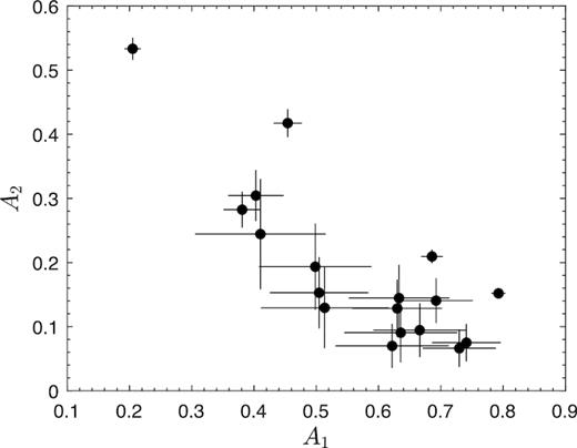
Correlation between A1 and A2.
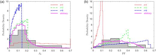
Distributions of (a)A2 and (b) PF for observed and simulated pulse profiles. The grey histograms are the observed distributions. We overplot the histograms of simulated pulsed profiles for two hotspots with intensity ratios of r = 1 (red dotted line), r = 3 (green dashed line), r = 9 (blue dash–dotted line), and arbitrary intensity ratios between 1 and 6 (solid magenta line).
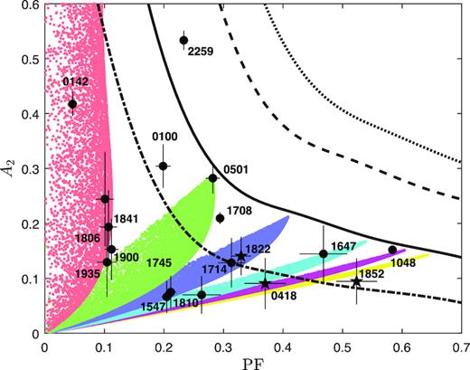
A2 versus PF for observed and simulated profiles. The dots and stars are observed values (see Table 2), with the latter indicating low-B-field magnetars. Error bars denote 1σ uncertainties. The red, green, blue, cyan, magenta and yellow points are the simulated data points for intensity ratios between two hotspots of 1 (symmetric), 2, 3, 5, 7 and 9, respectively. The beaming is calculated using the Hopf function. The thick solid line represents the maximum available A2 and PF for the given Hopf beaming. The dotted, dashed, and dash–dotted lines represent strong beaming with cos3θ′, the beaming function adopted from van Adelsberg & Lai (2006), and the isotropic emission, respectively (see Appendix C).
4.2 Correlation with physical parameters
We further investigate the correlation between pulse-profile parameters and physical parameters. Figs 6(a) and (b) show the age dependence of A2 and PF. Four magnetars, CXOU J1714, 1E 1841, SGR 0501 and 1E 2259, have well-measured SNR ages that are much younger than their τc (Leahy & Tian 2007; Nakamura et al. 2009; Tian & Leahy 2008; Sasaki et al. 2013). We plotted them on the same figure for comparison. A2 has no clear correlation. On the other hand, PF has an intriguing age dependence. However, the correlation analysis does not yield a significant linear correlation, with a null hypothesis probability of 0.4. Considering that the correlation could be non-linear, we calculated Spearman’s rank correlation and found a coefficient of 0.5 with a null hypothesis probability of 0.04, only slightly higher than 2σ significance. We further plotted the B-field dependence of A2 and PF in Figs 6(c) and (d) to check if there is any correlation, although the spin-down-inferred B field contains only the dipolar term. The distributions are similar to a horizontal flip of those with respect to τc because the spin period of magnetars is distributed in a narrow range (see e.g. Ho 2013). Both the Pearson and the Spearman correlation analysis yield a weak anticorrelation between PF and the B field, with a coefficient of ∼−0.5 and a null hypothesis probability of 0.05 (Pearson) and 0.01 (Spearman).
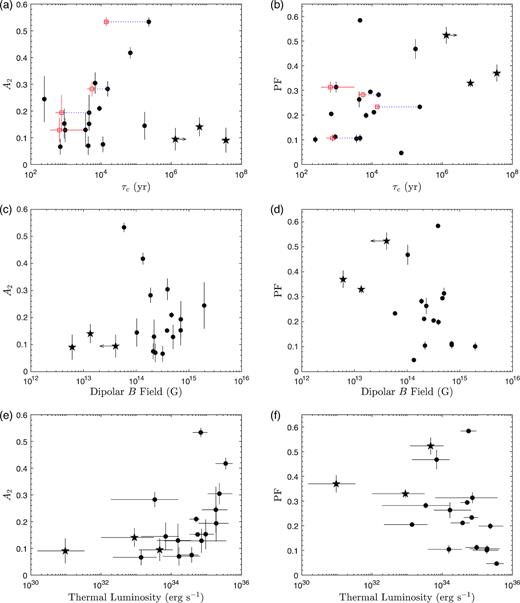
A2 and PF versus τc, the B field, and the thermal luminosity. The star symbols refer to the low-B-field magnetars. The error bars denote 1σ uncertainties for A2 and PF. The uncertainties of the thermal luminosity are from the 90 per cent confidence interval through spectral fitting in the literature and the distance measurements. They are dominated by the assumed 50 per cent distance uncertainty (see text). Four magnetars with well-measured SNR ages (CXOU J171405.7 − 381031, 1E 1841 − 045, SGR 050 + 4516 and 1E 2259 + 586) are further denoted by red squares and connected to their τc with blue dotted lines.
Magnetars are believed to have complex B-field structures that cannot be inferred solely from spin-down. The thermal luminosity could provide hints about the hidden fields according to the magneto-thermal evolution model. Therefore, we examined the thermal luminosity dependence of A2 and PF, as shown in Figs 6(e) and (f). We found a weak correlation between A2 and the thermal luminosity, with a null hypothesis probability of 0.01 (Pearson) and 0.008 (Spearman). PF weakly anticorrelates with the thermal luminosity, and both correlation analysis methods suggest a correlation coefficient of ∼− 0.6 and a null hypothesis probability of 0.01. This is expected because the dipolar B field of magnetars positively correlates with the X-ray luminosity (An et al. 2012; Mong & Ng 2018).
5 SIMULATION OF PULSE PROFILES
In the soft X-ray band, the emission is dominated by the thermal radiation from the surface. The pulse profiles therefore reflect the anisotropy of the surface temperature distribution. Theoretical works suggest that the temperature profile could show localized hotspots or an asymmetric pattern (Viganò et al. 2013; Gourgouliatos, Wood & Hollerbach 2016). In practice, the surface temperature profile and the emission geometry of a few magnetars were constrained by using models consisting of two antipodal hotspots with different intensities, for example for SGR 0418 + 5729 (Guillot et al. 2015), XTE J1810 – 197 (Perna & Gotthelf 2008; Bernardini et al. 2011) and PSR J1119 – 6127 (Ng et al. 2012). We applied the same method as described in DeDeo et al. (2001) to our sample of magnetars. We also note that the viewing geometry plays a critical role in the observed profiles. For two hotspots located at the magnetic poles, the observed pulse profile could be single-peaked, double-peaked, or even quadruple-peaked depending on the line of sight (see e.g. Ho 2007). It is possible to test the surface temperature anisotropy of magnetars in a statistical way with simulations of different viewing geometries.
We first assumed a symmetric surface intensity distribution with respect to the magnetic equator, namely two antipodal hotspots with the same size and intensity. We adopted an analytical form of the intensity for a hotspot described by equation (C1) and generated 104 sets of randomly distributed α (the angle between the rotation and magnetic axes) and ζ (the angle between the rotational axis and the line of sight). We assumed the Hopf beaming function (Chandrasekhar 1950) and calculated the pulse profiles (see Appendix C for the detailed calculation). The gravitational light-bending effect was approximated using the analytical formula derived by Beloborodov (2002). We then calculated A2 and PF from all the simulated profiles. The resulting probability density distributions are plotted in Fig. 4. A2 is almost uniformly distributed between 0 and 0.7, while PF is strongly concentrated below ∼0.12.
We then followed the procedure described in DeDeo et al. (2001) to tune the intensity ratios, r, between two hotspots from 1 to 9. For each set of r, we fixed one hotspot with a profile described by equation (C1), and set the intensity of the other hotspot by multiplying the same equation by r. Then we performed 104 Monte Carlo simulations of different viewing geometries. We plot three cases, r = 1, r = 3 and r = 9, in Fig. 4. Not surprisingly, the distributions for r = 3 and r = 9 show low A2 ≲ 0.2, while that for r = 1 shows a flat distribution because the asymmetric surface intensity profile tends to result in a single-peaked profile. PF shows a relatively broad distribution for r = 3 and r = 9, although profiles with high PF are slightly more probable in both cases. The sharp distribution for r = 1 at |$\rm {PF}\lesssim 0.1$| indicates that symmetric antipodal hotspots never result in a pulse profile with a high PF. These three distributions are far from the observed one. We found that if we performed a simulation with a choice of randomly distributed r between 1 and 6, and randomly distributed α and ζ, the resulting distribution of A2 and PF can roughly reproduce the observed distribution. This implies that the surface temperature distribution of magnetars varies greatly from source to source.
Fig. 5 shows PF versus A2 for simulated profiles compared with observed ones. For the case of two symmetric hotspots, PF is systematically low and A2 spreads over a large range. As r increases, the maximum allowed A2 decreases and PF increases. For an assumed beaming function, no system is allowed to lie above the upper envelope of the distribution. We also plotted the envelopes for the cases of isotropic emission without beaming, the beaming effect in van Adelsberg & Lai (2006), and the strongest beaming of cos3θ′ (see Appendix C). We tried different degrees of concentration of hotspots by changing the numerator in equation (C1) as cosnθm and tuning n from n = 2 (least concentrated, equivalent to a large hotspot) to n = 8 (most concentrated, equivalent to a small hotspot). We found that more concentrated hotspots with weaker beaming show similar behaviours of a less concentrated hotspot with a stronger beaming function. Only ∼50 per cent of the sample is below the envelope of isotropic emission, indicating that atmospheric beaming is necessary. Most magnetars can be interpreted by the Hopf beaming function, except for 1E 2259. This object could have more concentrated hotspots or a beaming function stronger than the Hopf function. All magnetars are enclosed by the envelope of strong beaming functions. Moreover, a profile with both high A2 and high PF needs two extremely small hotspots with strong atmospheric beaming. None of the magnetars in our sample shows these properties.
The above simulations suggest that the viewing geometry dominates the observed A2 and PF. Hence, we estimated the degree of asymmetry for our sample of magnetars by obtaining the possible range of r based on the simulation. We set up a 1000 × 1000 × 1000 grid on α, ζ, r, and created simulated profiles by assuming a Hopf beaming. We obtained the distribution of allowed α, ζ and r that can produce the observed A2 and PF of individual magnetars within the uncertainties. The distribution of r is shown in Fig. 7. Six magnetars, SGR 0418, 1E 1547, CXOU J1647, SGR 1745, XTE J1810 and 3XMM J1852, have wide distributions truncated at the limit of r = 9 in the simulation. Otherwise, their probability distribution of r could extend to much higher values. We found that eight magnetars, CXOU J0100, 4U 0142, SGR 0501, 1RXS J1708, SGR 1806, 1E 1841, SGR 1900 and SGR 1935, have well-constrained r ≲ 3. 1E 1048 has a well-constrained r between 6 and 7. CXOU J1714 and Swift J1822 have a moderately constrained r between 2 and 6. 1E 2259 is not included in Fig. 7 because the observed A2 and PF (see Fig. 5) is beyond the limits of the simulation based on our assumptions. However, a low value of r is expected owing to its high A2 and low PF.
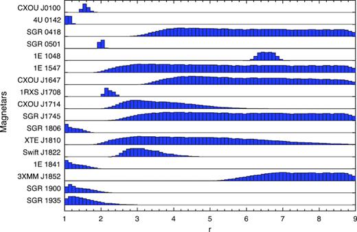
Distribution of the intensity ratio between two hotspots for magnetars. The probability densities are scaled to have identical peak heights for display purposes.
We estimated the median value of the distribution for individual magnetars as the r value and treated the boundaries of the distribution as the uncertainty intervals. The inferred values of r are plotted against τc in Fig. 8(a). The plot shows no obvious correlation and no pattern similar to that in Fig. 6. This suggests that the apparent evolutionary pattern in Fig. 6(a) could be merely a coincidence. We also plotted the thermal luminosity dependence of r in Fig. 8(b) and found a similar distribution to the PF–luminosity plot. The linear correlation coefficient between r and luminosity is −0.57 with a null hypothesis probability of 0.009, while Spearman’s rank correlation suggests a similar coefficient of −0.64 and a slightly more significant probability of 0.006. We cannot draw a strong conclusion for the linear correlation but a systematic trend probably exists. This implies that magnetars with high luminosities tend to have symmetric surface intensity profiles. It is necessary to include more magnetars to unambiguously confirm this correlation with the next generation of X-ray observatories.
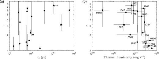
Correlation between the inferred intensity ratio r between two hotspots and (a) τc and (b) the thermal luminosity. The star symbols refer to the low-B-field magnetars. The error bar of r is calculated from the full range of the distribution in Fig. 7.
6 DISCUSSION
We found that those magnetars with intensity ratio r ≲ 3 are young objects, except for 4U 0142. 1E 2259 is also probably in this category because it shows a high A2 and relatively low PF, although a stronger beaming function or a smaller hotspot is necessary. The SNR age of 1E 2259 is 14 kyr, much younger than its τc = 230 kyr, and this object can still be classified as a young magnetar. 4U 0142 could have a similar young age, because its luminosity is extremely high, but further investigation of its true age is needed. In contrast, other magnetars may need high surface temperature asymmetry, although some of them have large error bars and r < 3 remains possible. We are unable to draw strong conclusions about their surface temperature anisotropy. All the low-B-field magnetars with large τc are classified in this category. They could be evolved magnetars in which the B field has decayed to the current low value and in which the symmetry has been broken. 1E 1048 is an intriguing case in that the viewing geometry can be well constrained. It has a low τc = 4.5 kyr and a high spin-down-inferred B = 3.9 × 10¹⁴ G, so is much younger and more luminous than those low-B-field magnetars showing similar pulse profile properties. These behaviours could provide a hint of the initial B-field strength of magnetars. The Hall drift breaks the symmetry of the surface temperature distribution on a shorter time-scale for a stronger B field. As one of the eight extreme magnetars characterized by large |$\dot{P}$| and high initial magnetic fields, 1E 1048 has the lowest thermal luminosity (Viganò et al. 2013). Therefore, it is probably an evolved extreme magnetar, and the symmetry was broken faster than in other magnetars with lower initial magnetic fields.
Alternatively, these outliers could be interpreted as arising from the effect of relatively small-scale hotspots on the NS surface. These hotspots can be generated by interior magnetic field structures composed of a mixture of dipolar and toroidal components, and could produce large PF, A2, and/or hotspot asymmetry r. The generation and the persistence of these small-scale structures are attributed to Hall drift, which causes the movement of the B field to regions of lower conductivity and subsequent enhancement of field dissipation and heating. These hotspots can grow quickly and persist for a long time, as demonstrated by numerical simulations of B-field evolution that are sometimes coupled to thermal evolution simulations. For example, Geppert & Viganò (2014) found rapid development (on a time-scale of ∼104 yr) of substantial tens-of-degree surface regions with the magnetic field and temperature exceeding global averages, and these regions can last for >106 yr. Similarly, Gourgouliatos et al. (2016) and Gourgouliatos & Hollerbach (2018) found kilometre-size magnetic spots whose field strengths can greatly exceed the dipolar B field at the pole. However, it is important to keep in mind that the development of these magnetic field structures depends strongly on the initial magnetic field configuration, which is not uniquely prescribed, and requires a toroidal component at least as strong as the dipolar component (c.f. Kojima & Kisaka 2012).
7 SUMMARY
We have carried out a comprehensive investigation of the quiescent soft X-ray pulse profiles of magnetars by calculating the strength of the Fourier components and PF. We find that over half of our sample of magnetars have low amplitudes of the second Fourier harmonic and low PF, while the others have either high A2 or high PF. We further performed simulations to explore the surface temperature distribution by assuming two hotspots with different intensities. We find that the viewing geometry dominates the shape of the observed pulse profiles, and a diversity of the intensity ratio between two hotspots is needed to explain the observed distribution of A2 and PF. The correlation analysis shows intriguing dependences between the profile shape and the physical parameters, including τc, the dipolar B field, and the thermal luminosity. We estimated the intensity ratio between two hotspots by comparing the profile parameters from the magnetar sample and the simulations. We suggest that the surface temperature symmetry correlates with the thermal luminosity; that is, magnetars with higher luminosity generally have more symmetric profiles with respect to the magnetic equator. This can be interpreted as the result of evolution if all the magnetars have strong toroidal fields and the symmetry between two hotspots is destroyed through evolution.
In addition to the main result, we updated the long-term spin-period evolution of CXOU J1714 with four more data sets after the latest reports. The result shows |$\dot{P}=(6.41\pm 0.03)\times 10^{-11}$| s s−1 over a time span of ∼7 yr, consistent with that obtained from the first two Chandra and XMM–Newton observations.
ACKNOWLEDGEMENTS
We sincerely thank the referee for valuable suggestions on the paper. This research is in part based on the data obtained from the Chandra Data Archive, and has made use of software provided by the Chandra X-ray Center (CXC) in the application packages ciao, ChIPS, and Sherpa. This research has used observations obtained with XMM–Newton, and the ESA science mission, with instruments and contributions directly funded by ESA Member States and NASA. C-PH and C-YN are supported by a GRF grant from the Hong Kong Government under HKU 17300215P. WCGH acknowledges support from STFC in the UK through Grant No. ST/M000931/1.
Footnotes
REFERENCES
APPENDIX A: SPIN-PERIOD EVOLUTION OF CXOU J171405.7 – 381031
Currently, the most reliable measurement of the spin-down rate of CXOU J1714 is |$\dot{P}=(6.40\pm 0.05)\times 10^{-11}$| s s−1, utilizing Chandra and XMM–Newton observations in 2009–2010 (time span ∼1.1 yr). Because three more Chandra observations (ObsIDs 13749, 16762, 16763) and one XMM–Newton observation (ObsID 0670330101) have been made since the latest reported |$\dot{P}$|, we performed the H test to search for periodicity from all available Chandra and XMM–Newton data to update the ephemeris. The evolution of the spin period is shown in Fig. A1, where the linear fit implies a period derivative of |$\dot{P}=(6.41\pm 0.03)\times 10^{-11}$| s s−1 over a time span of ∼7 yr. This value is consistent with that determined by Sato et al. (2010). Moreover, the fitting is poor, with a χ2/dof = 350/5, and a significant discrepancy between individual data points and the long-term evolutionary trend is clearly seen. The difference is particularly large near ∼MJD 56000, where a timing anomaly event probably occurred.
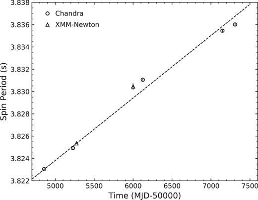
Spin-period evolution of CXOU J171405.7 – 381031 obtained with Chandra and XMM–Newton.
APPENDIX B: THERMAL LUMINOSITIES OF QUIESCENT MAGNETARS
The emission of most magnetars shows two thermal components: a low-temperature component from the entire surface and a high-temperature component from the hotspots. The parameters of the low-temperature component are sometimes not well determined (Mong & Ng 2018, and references therein). We calculated the bolometric thermal luminosities from both components for those magnetars with well-constrained parameters from Mong & Ng (2018). Otherwise, we calculated the luminosities using a single blackbody (BB) model. We further fitted the X-ray spectra of SGR 0418, SGR 1745, 3XMM J1852 and SGR 1935 extracted from the data sets listed in Table 1 to constrain their spectral parameters and the thermal luminosities in quiescence. We used Sherpa (Freeman, Doe & Siemiginowska 2001) to fit the X-ray spectra. The absorption model we used in the spectral analysis was 'tbnew'.5 We set the interstellar abundance according to Wilms, Allen & McCray (2000), which uses the cross-section presented in Verner et al. (1993). In case of multiple observations of a single source, we set the parameters to be the same between data sets because no significant variabilities were found. We fitted the Chandra spectra in 0.5–7 keV and the XMM–Newton spectra in 0.3–10 keV with the Cash statistic (Cash 1979). We used a simple BB to characterize the thermal component and added a power-law component when necessary. Adding another BB component is not necessary for these four sources. The results for SGR 0418, SGR 1745 and 3XMM J1852 are consistent with the literature (Rea et al. 2013; Coti Zelati et al. 2017; Zhou et al. 2014). The spectral behaviour of SGR 1935 in the new XMM–Newton data set was not reported in the literature. We fitted the spectra and found that adding a power-law component can greatly improve the fit statistic. The maximum likelihood ratio test suggests a null hypothesis probability of 10−52. The temperature is consistent with previous Chandra observations (Israel et al. 2016). The thermal luminosities of all the magnetars are summarized in Table 2. The best-fit spectral parameters, including the hydrogen column density (|$N_{\textrm{H}}$|), BB temperature (|$kT_{\textrm{BB}}$|),the normalization factor of BB, and the photon index (|$\Gamma$|) are listed in Table B1.
APPENDIX C: MODELLING THE PULSE PROFILE
We integrated equation (C4) over the visible surface with cos ψ > −rs/(R − rs) to obtain the pulse profile. Four typical profiles are shown in Fig.C1: class I (α = 20 °, ζ = 30 °), class II (α = 30 °, ζ = 60 °), class III (α = 60 °, ζ = 80 °) and class IV (α = 80 °, ζ = 20 °) . For the case of symmetric hotspots, the pulse profile is single-peaked for class I and class II, while it becomes double-peaked for class III and class IV. Moreover, PF is enhanced as a result of the beaming effect. We also plotted the extreme case that one hotspot is nine times brighter than another. In this case, the profiles are all single-peaked with lower A2 and higher PF compared with the symmetric case.
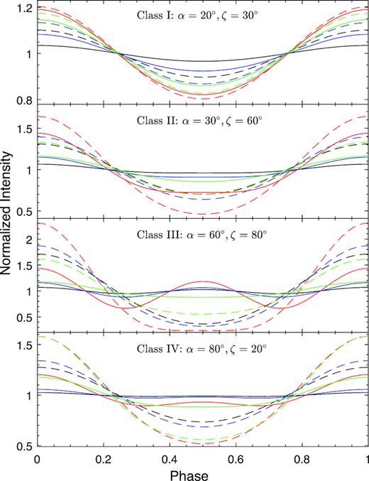
Simulated pulse profiles for different α and ζ. The solid profiles are from two hospots with equal brightness, while the dashed profiles are from two asymmetric hotspots in which one is nine times brighter than the other. The black, blue, red, and green curves are calculated from the isotropic emission, mild beaming from the Hopf function, strong beaming as cos3θ′, and the beaming function adopted from van Adelsberg & Lai (2006).
To further test the available PF and A2 from the asymmetric surface temperature profile, we tuned the different intensity ratio emerging from two hotspots from 1 to 9 and performed Monte Carlo simulations. For each assumed intensity ratio, we generated 104 sets of randomly distributed α and ζ, and calculated their pulse profiles, PFs and A2. The results are plotted in Fig. 5. The envelope denotes the available A2 and PF area with the brightness function described in equation (C1) with different beaming functions. We performed the same simulations for the case of more concentrated hotspots and found that the effect is similar to a stronger beaming.
Author notes
JSPS International Research Fellow.
