High-order magnetohydrodynamics for astrophysics with an adaptive mesh refinement discontinuous Galerkin scheme

Guillet, Thomas; Pakmor, Rüdiger; Springel, Volker; Chandrashekar, Praveen; Klingenberg, Christian

doi:10.1093/mnras/stz314

Abstract

Modern astrophysical simulations aim to accurately model an ever-growing array of physical processes, including the interaction of fluids with magnetic fields, under increasingly stringent performance and scalability requirements driven by present-day trends in computing architectures. Discontinuous Galerkin (DG) methods have recently gained some traction in astrophysics, because of their arbitrarily high order and controllable numerical diffusion, combined with attractive characteristics for high-performance computing. In this paper, we describe and test our implementation of a DG scheme for ideal magnetohydrodynamics (MHD) in the arepo-dg code. Our DG-MHD scheme relies on a modal expansion of the solution on Legendre polynomials inside the cells of an Eulerian octree-based adaptive mesh refinement grid. The divergence-free constraint of the magnetic field is enforced using one out of two distinct cell-centred schemes: either a Powell-type scheme based on non-conservative source terms, or a hyperbolic divergence cleaning method. The Powell scheme relies on a basis of locally divergence-free vector polynomials inside each cell to represent the magnetic field. Limiting prescriptions are implemented to ensure non-oscillatory and positive solutions. We show that the resulting scheme is accurate and robust: it can achieve high-order and low numerical diffusion, as well as accurately capture strong MHD shocks. In addition, we show that our scheme exhibits a number of attractive properties for astrophysical simulations, such as lower advection errors and better Galilean invariance at reduced resolution, together with more accurate capturing of barely resolved flow features. We discuss the prospects of our implementation, and DG methods in general, for scalable astrophysical simulations.

hydrodynamics, MHD, shock waves, methods: numerical

1 INTRODUCTION

Numerical simulations in astrophysics have established themselves as a critical tool to study the complex interactions of physical processes in the Universe. Galaxy formation simulations, in particular, are faced with the challenge of accounting for ever expanding models of the physics, while requiring increasingly accurate numerical methods and scalable high-performance implementations.

Among these physical processes, cosmic magnetic fields are now recognized as playing a key role in star formation in the interstellar medium, and possibly impacting the dynamics of gas in galaxies at larger scales as they get amplified by multiple dynamo processes which are still only partially understood. For this reason, many astrophysical codes have been implementing magnetohydrodynamics (MHD) solvers, to compute the joint evolution of gas and magnetic fields (e.g. Stone & Norman 1992; Fryxell et al. 2000; Fromang, Hennebelle & Teyssier 2006; Mignone et al. 2007; Stone et al. 2008; Collins et al. 2010; Pakmor, Bauer & Springel 2011). These methods have been applied to set-ups of growing physical complexity, from the study of magnetized turbulence in the interstellar medium (Stone, Ostriker & Gammie 1998; Mac Low 1999; Schekochihin et al. 2004; Federrath et al. 2010), to magnetic field evolution in isolated galaxy set-ups (e.g. Wang & Abel 2009; Dubois & Teyssier 2010; Pakmor & Springel 2013; Rieder & Teyssier 2016), and more recently, the amplification of magnetic fields in galaxies in full cosmological context (Pakmor, Marinacci & Springel 2014; Pakmor et al. 2017; Rieder & Teyssier 2017).

The increasing CPU and memory requirements of these simulations are confronted today by modern trends in computing architectures. It is now well recognized that advances in computing power are more due to the power-efficient integration of multiple processor cores, rather than single-core performance growth. In addition, memory technology has not been keeping up with the steady gains in floating-point computing power, lagging behind both in terms of performance and capacity. As a result, codes have to turn towards increasingly parallel and compute-efficient numerical methods to face the expanding computing and memory requirements of the physical models they attempt to simulate.

In recent years, discontinuous Galerkin (DG) methods have gained traction in the computational fluid dynamics community in general, and in astrophysics in particular, as a promising framework for scalable and accurate high-order methods for hyperbolic problems. DG schemes lie at the crossroads of spectral element and finite-volume methods: based on the expansion of the solution inside simulation volumes on a set of chosen basis functions (typically polynomials), DG schemes evolve the expansion coefficients (the so-called weights) in time based on a weak formulation of the governing equations. The popularity of DG stems from the fact that it provides a clean framework for discretizing hyperbolic problems at any order of spatial accuracy, together with attractive data locality: regardless of spatial order, DG schemes in theory require communication only between directly neighbouring cells, unlike high-order reconstruction-based finite-volume methods. As a result, DG methods have been the focus of intense research over the last three decades (see e.g. Cockburn & Shu 1989, 1998; Cockburn, Li & Shu 2004; Li & Shu 2005; Hesthaven & Warburton 2008; Li, Xu & Yakovlev 2011; Shu 2013; Balsara 2017).

Because DG methods can easily be set-up to operate at any spatial order, their numerical dissipation is controllable and can be reduced as required, which is of great interest to simulate the high Reynolds number flows of astrophysical plasmas. From a pure hydrodynamics point of view, Bauer & Springel (2012) and Nelson et al. (2013) show that numerical dissipation can result in spurious heating of the intergalactic medium from turbulent motions, preventing cooling and accretion of the hot ambient gas. This result is corroborated by Zhu et al. (2013) in the context of higher order reconstruction-based methods. In the context of decaying isothermal magnetized supersonic turbulence, the code comparison study of Kritsuk et al. (2011) has shown that higher order codes provide a larger turbulence spectral bandwidth and increased effective Reynolds number compared to second-order schemes. Even at second order, recent studies by Mocz et al. (2014) and Schaal et al. (2015) show that DG methods demonstrate overall superior accuracy compared to finite-volume methods, in particular due to lower advection errors and reduced angular momentum diffusion. Beyond second order, Schaal et al. (2015) find that, on smooth problems at least, increasing the DG order reduces advection errors, and decreases the total time-to-solution for a given target accuracy.

These properties make DG schemes attractive for fixed grid Eulerian astrophysical codes, where large structures such as galaxies may travel across the grid with large bulk advection velocities. As a result, there has been significant recent interest in DG methods in astrophysics, for hydrodynamics (Schaal et al. 2015; Velasco Romero et al. 2018), ideal MHD (Mocz et al. 2014; Dumbser & Loubère 2016; Karami Halashi & Luo 2016), non-ideal MHD (Boscheri & Dumbser 2017), as well as special- and general-relativistic MHD (Zanotti, Fambri & Dumbser 2015; Kidder et al. 2017; Anninos et al. 2017; Zhao & Tang 2017; Fambri et al. 2018).

In this paper, we present arepo-dg, our extension of the hydrodynamical DG code tenet of Schaal et al. (2015), to ideal MHD. Like its predecessor, this work leverages the infrastructure of the moving mesh code arepo (Springel 2010), but instead of a moving Voronoi mesh, relies on arepo’s optional support for fixed Eulerian adaptive grids. The goal is to develop new parallel Eulerian solvers within this existing framework which explores different accuracy and scalability compromises than the moving mesh solution.

Our code adopts a modal Legendre polynomial basis for the expansion of hydrodynamical variables. Two different methods are implemented to control the divergence of the magnetic field: in a first scheme, which we refer to as the Powell method, the magnetic field components are expanded within each cell on to a special basis of locally divergence-free (LDF) vector polynomials (Cockburn et al. 2004; Li & Shu 2005; Yakovlev, Xu & Li 2013; Zhao, Yang & Seyler 2014; Zhao & Tang 2017), and additional source terms are introduced following the formulation of Powell et al. (1999). For this Powell method, the LDF basis only ensures that the magnetic field is locally divergence-free inside a cell, but not globally divergence-free, since the normal component of the magnetic field is not guaranteed to be continuous across cell interfaces. The other implemented divergence control method relies on hyperbolic divergence cleaning as formulated by Dedner et al. (2002), for which we typically use the same Legendre basis both for hydrodynamical variables and the magnetic field components. With this scheme and choice of basis, the magnetic field is formally neither locally nor globally divergence-free, but its divergence is instead dynamically damped and advected away using an additional scalar field.

The DG weights are evolved in time through explicit time integration of the semidiscrete scheme, in the so-called Runge–Kutta DG (RKDG) framework introduced by Cockburn, Lin & Shu (1989). In this paper, we discuss our implementation, detailing the numerical ingredients required for code stability and accuracy, with a special focus on the treatment of the divergence of the magnetic field. Our scheme introduces two new elements: different discretizations of the Powell term in the DG framework in Section 4.1.3, and a non-linear divergence-free slope limiting procedure for the magnetic field in Section 4.2.4. We also cover some important aspects of the method related to performance and computing efficiency.

This paper is organized as follows. In Section 2, we review the governing equations for ideal MHD in their conserved formulation. In Section 3, we describe our DG discretization and time integration scheme, with a focus on aspects specific to MHD, in particular the divergence-free basis for the Powell scheme. Section 4 details the numerical ingredients required to make the scheme accurate and stable with MHD; we discuss in particular the issues related to oscillation limiting, control of the divergence of the magnetic field, and enforcement of solution positivity. In Section 5, we present results on a number of test problems, showing that the method achieves high order in smooth regions, while capturing shocks and discontinuities. We show that higher orders indeed reduce advection errors and dissipation even in case of strong MHD shocks, and help to efficiently capture barely resolved flow features. We also present test problems specifically aimed at testing the control of the magnetic field divergence. In Section 6, we discuss prospects for this method and astrophysical simulations, also covering some aspects related to implementation efficiency and performance. We also consider some challenges and future prospects for our scheme – and DG methods in general – towards large-scale production astrophysical simulations.

2 GOVERNING EQUATIONS

The ideal MHD equations may be written as a system of conservation laws of the form:

\begin{eqnarray*} \frac{\partial \boldsymbol u}{\partial t} + \sum _{\alpha =1}^{3} \frac{\partial \boldsymbol f_\alpha (\boldsymbol u)}{\partial x_\alpha } = 0, \end{eqnarray*}

(1)

where the index α runs over all space dimensions. The vector |$\boldsymbol u$| holds the conserved variables of the system:

\begin{eqnarray*} \boldsymbol u= {\left[\begin{array}{c}\rho \\ \rho \boldsymbol v\\ E \\ \boldsymbol B\end{array}\right]}, \quad E = \rho u + \frac{1}{2}\rho \boldsymbol v^2 + \frac{1}{2}\boldsymbol B^2, \end{eqnarray*}

(2)

where ρ is the density, |$\boldsymbol v$| the fluid velocity, E the total energy density, |$\boldsymbol B$| the magnetic field vector, p the hydrodynamic (thermal) pressure, and u is the specific internal energy, which we assume to be related to the pressure p by the ideal gas equation of state with adiabatic index γ:

\begin{eqnarray*} p = \rho u (\gamma - 1), \end{eqnarray*}

(3)

from which we will write the total energy as

\begin{eqnarray*} E = \frac{p}{\gamma -1} + \frac{1}{2}\rho \boldsymbol v^2 + \frac{1}{2}\boldsymbol B^2. \end{eqnarray*}

(4)

The fluxes |$\boldsymbol f_\alpha (\boldsymbol u)$| for ideal MHD are given by

\begin{eqnarray*} \boldsymbol f= {\left[\begin{array}{c}\rho \boldsymbol v\\ \rho \boldsymbol v\otimes \boldsymbol v+ p_\mathrm{ T}\mathcal {I}_3 - \boldsymbol B\otimes \boldsymbol B\\ (E + p_\mathrm{ T}) \boldsymbol v- ({\boldsymbol v}{\cdot }{\boldsymbol B}) \boldsymbol B\\ \boldsymbol B\otimes \boldsymbol v- \boldsymbol v\otimes \boldsymbol B\end{array}\right]}, \end{eqnarray*}

(5)

where |$\mathcal {I}_3$| is the 3 × 3 identity matrix, and p_T is the total pressure defined by

\begin{eqnarray*} p_\mathrm{ T}= p + \frac{1}{2}\boldsymbol B^2. \end{eqnarray*}

(6)

For physical solutions, the Maxwell equations impose the additional constraint

\begin{eqnarray*} {\nabla }{\cdot }{\boldsymbol B}= 0 \end{eqnarray*}

(7)

everywhere and at all times. The form of the flux (5) guarantees that initial divergence-free solutions will remain divergence-free under the dynamical evolution dictated by equation (1). However, this is not necessarily true for approximate numerical solutions, which require special divergence control measures.

3 DISCONTINUOUS GALERKIN SCHEME

We now describe our DG scheme, which follows the overall RKDG framework of Cockburn et al. (1989) and Cockburn & Shu (1989). The implementation adopts the general set-up of Schaal et al. (2015), but is adapted to MHD. In the following, we present the more general case of the Powell divergence control scheme, which relies on a basis of locally divergence-free polynomials for the magnetic field components (Cockburn et al. 2004; Li & Shu 2005; Yakovlev et al. 2013). The other divergence control scheme, hyperbolic cleaning, requires only the use of the Legendre basis. We discuss both implementations of divergence control in Section 4.1.

3.1 Representation of the conserved state

The computational domain is partitioned into non-overlapping cubic cells, structured as an adaptive mesh refinement (AMR) octree. Within each cell K, the local conserved state vector |$\boldsymbol u^K(\boldsymbol x,t)$| is expanded as a linear combination of N time-independent basis functions |$\boldsymbol \phi_{l}^K(\boldsymbol x)$|⁠, defining time-dependent weights |$w_{l}^K(t)$|⁠:

\begin{eqnarray*} \boldsymbol u^K(\boldsymbol x,t) = \sum _{l=1}^N w^K_{l}(t) \boldsymbol \phi_{l}^K(\boldsymbol x). \end{eqnarray*}

(8)

For each basis index l, |$\boldsymbol \phi_{l}^K$| is a vector of eight time-independent scalar fields over K, one for each conserved component, and |$w_{l}^K(t)$| is a time-dependent scalar function.

The weights |$w^K_{l}$| are defined independently in each cell, resulting in fields which are discontinuous at interfaces. Since all cells are cubic, we can define reference basis functions |$\boldsymbol \phi_{l}$| independent of cell K by simple translation and rescaling of world coordinates |$\boldsymbol x$| to reference cell coordinates |$\boldsymbol \xi \in [-1, 1]^3$|⁠:

\begin{eqnarray*} \boldsymbol \phi _{l}^K(\boldsymbol x) = \boldsymbol \phi _{l}(\boldsymbol \xi), \qquad \boldsymbol \xi = \frac{2}{\Delta x^K}\left(\boldsymbol x- \boldsymbol x_\mathrm{ c}^K\right) \end{eqnarray*}

(9)

where |$\Delta x^K, \boldsymbol x_\mathrm{ c}^K$| are the cell size and cell centre in world coordinates.

We further define the L² inner product on conserved vector fields in the reference cell:

\begin{eqnarray*} \left\langle {\boldsymbol u_1},{\boldsymbol u_2}\right\rangle {:=} \int _{[-1,1]^3} {\boldsymbol u_1(\boldsymbol \xi)}{\cdot }{\boldsymbol u_2(\boldsymbol \xi)} \,\, \mathrm{d} \boldsymbol \xi , \end{eqnarray*}

(10)

where the dot product on the right-hand side is the usual dot product of |$\mathbb {R}^8$|⁠, i.e. across conserved components. By choosing a set of basis functions orthogonal with respect to this inner product, we can readily invert equation (8) by taking the inner product against each basis function:

\begin{eqnarray*} w^K_{ l}(t) = M_{ l}^{-1} \left\langle {\boldsymbol u^K},{\boldsymbol \phi _{ l}}\right\rangle , \end{eqnarray*}

(11)

where

\begin{eqnarray*} M_{ l} {:=} \left\langle {\boldsymbol \phi _{ l}},{\boldsymbol \phi _{ l}}\right\rangle \end{eqnarray*}

(12)

is the diagonal of the mass matrix |$\left\langle {\boldsymbol \phi _{ l}},{\boldsymbol \phi _{{ l}^{\prime }}}\right\rangle$|⁠, all non-diagonal entries being zero. We now discuss the two types of basis functions making up our global DG basis |$\lbrace \boldsymbol \phi _{ l}\rbrace , l \in \lbrace 1,\ldots ,N\rbrace$|⁠.

3.2 Legendre basis for hydrodynamics

Following Schaal et al. (2015), we expand the hydrodynamical variables ρ, |$\rho \boldsymbol v$|⁠, and E independently on to five scalar Legendre polynomials of degree ≤d. In three dimensions, scalar trivariate Legendre polynomials are indexed by three integers k₁, k₂, k₃ with k₁ + k₂ + k₃ ≤ d, and take the form:

\begin{eqnarray*} P_{k_1,k_2,k_3}(\boldsymbol \xi) = \ell _{k_1}(\xi _1) \ell _{k_2}(\xi _2) \ell _{k_3}(\xi _3), \quad k_1+k_2+k_3 \le d, \end{eqnarray*}

(13)

where ℓ_k is the univariate Legendre polynomial of degree k. The |$P_{k_1,k_2,k_3}$| form a basis of the space of scalar trivariate polynomials of degree ≤d, which has dimension

\begin{eqnarray*} n(d) = \frac{1}{6} (d+1)(d+2)(d+3). \end{eqnarray*}

(14)

For brevity, we collectively label (k₁, k₂, k₃) with a single integer in {1, …, n(d)}. Note that the univariate Legendre polynomials ℓ_k are orthogonal for the L² inner product on [−1, 1]:

\begin{eqnarray*} \int _{[-1,1]} \ell _{{ k}}(x) \ell _{{ k}^{\prime }}(x) \, \mathrm{d}x = 0 \Leftrightarrow k \ne k^{\prime }, \end{eqnarray*}

(15)

and as a result, the polynomials of equation (13) are orthogonal for the same inner product on the reference cell [−1, 1]³.

Since we are expanding five conserved components independently, the Legendre subset of our basis functions will have dimension N_L = 5n(d). We can choose the basis indexing l so that the first n(d) components l ∈ {1, …, n(d)} correspond to the Legendre expansion of ρ, then l ∈ {n(d) + 1, …, 2n(d)} correspond to ρv₁, etc. To write the Legendre |$\boldsymbol \phi _{ l}$| explicitly in terms of vectors of conserved components:

\begin{eqnarray*} \boldsymbol \phi _{{ l}}(\boldsymbol \xi) = {\left[\begin{array}{c}P_{{ l}}(\boldsymbol \xi) \\ \boldsymbol 0 \\ 0 \\ \boldsymbol 0 \end{array}\right]}, \ l \in \lbrace 1, \ldots , n(d)\rbrace , \quad \text{for }\rho \end{eqnarray*}

(16)

up to

\begin{eqnarray*} \boldsymbol \phi _{4n(d)+l}(\boldsymbol \xi) = {\left[\begin{array}{c}0 \\ \boldsymbol 0 \\ P_{{ l}}(\boldsymbol \xi) \\ \boldsymbol 0 \end{array}\right]}, \ l \in \lbrace 1, \ldots , n(d)\rbrace , \quad \text{for } E. \end{eqnarray*}

(17)

Since the multivariate Legendre polynomials P are L²-orthogonal, the |$\boldsymbol \phi$| we just constructed are orthogonal for the inner product (10).

3.3 Divergence-free basis for the magnetic field

LDF basis functions for DG techniques were first introduced by Cockburn et al. (2004) for the linear Maxwell equations, and extended by Li & Shu (2005) to non-linear MHD in the context of RKDG methods. Divergence-free bases have also been used for DG in the context of relativistic MHD by Zhao & Tang (2017). The idea is to enforce the divergence-free condition (7) inside the cells by expanding the magnetic field |$\boldsymbol B$| in equation (8) on to a basis of divergence-free vector polynomials, which in 3D has dimension:

\begin{eqnarray*} N_\text{div} = 3 n(d) - n(d-1). \end{eqnarray*}

(18)

We will discuss the properties of this basis for divergence control in Section 4.1, and we refer the reader to Appendix A for more details related to properties and constructions of such bases in 2D and 3D. In two dimensions, suitable basis functions may be found for example in Cockburn et al. (2004); Li & Shu (2005) up to d = 2, or Zhao & Tang (2017) up to d = 3.

The resulting total dimension of the DG basis with its Legendre and divergence-free subspaces is

\begin{eqnarray*} N = N_\text{L} + N_\text{div} = 8 n(d) - n(d-1). \end{eqnarray*}

(19)

Its general structure is represented in Fig. 1. As detailed in Appendix A, the divergence-free basis is constructed so that its vectors are orthogonal with respect to the inner product (10).

$Structure of the DG basis functions for 3D MHD with degree d = 1 polynomials, showing non-zero contributions (coloured cells) of each basis function $\boldsymbol \phi _{ l}$ (lth column) to components of the conserved state vector $\boldsymbol u$ (rows). The Legendre subspace for hydrodynamical variables has total dimension NL = 20, whereas the divergence-free subspace for $\boldsymbol B$ is of dimension Ndiv = 11. Cells in white correspond to zero. While the Legendre subspace has a tensor product structure, all three components of $\boldsymbol B$ in the divergence-free basis are coupled.$

Figure 1.

Structure of the DG basis functions for 3D MHD with degree d = 1 polynomials, showing non-zero contributions (coloured cells) of each basis function |$\boldsymbol \phi _{ l}$| (lth column) to components of the conserved state vector |$\boldsymbol u$| (rows). The Legendre subspace for hydrodynamical variables has total dimension N_L = 20, whereas the divergence-free subspace for |$\boldsymbol B$| is of dimension N_div = 11. Cells in white correspond to zero. While the Legendre subspace has a tensor product structure, all three components of |$\boldsymbol B$| in the divergence-free basis are coupled.

Open in new tab Download slide

The resulting combined Legendre and divergence-free basis is of dimension N = N_L + N_div, and is orthogonal:

\begin{eqnarray*} \forall (l, l^{\prime }) \in \lbrace 1,\ldots ,N\rbrace ^2, \quad \left\langle {\boldsymbol \phi _{ l}},{\boldsymbol \phi _{{ l}^{\prime }}}\right\rangle = \delta _{{ ll}^{\prime }} M_{ l}, \quad M_{ l} > 0, \end{eqnarray*}

(20)

which results from the block structure shown in Fig. 1, together with the orthogonality of the Legendre polynomials and divergence-free basis vectors. The constants M_l are fixed by the choice of basis polynomials.

LDF bases require slightly less storage per cell than expanding the components of |$\boldsymbol B$| as independent Legendre fields, due to the fewer degrees of freedom arising from the divergence constraint. However, we note that LDF bases prevent some optimizations that are possible with Legendre bases, thus requiring more floating point operations. They also require storing more precomputed data (such as the basis function values and gradients) compared to Legendre bases. We come back to these points in the discussion in Section 6.3.3.

3.4 The special case of 2D MHD

2D MHD problems can be seen as being governed by the 3D equations, but with imposed translation invariance along the third dimension of space, i.e. ∂/∂x₃ = ∂/∂ξ₃ ≡ 0. In this case, the divergence-free condition on |$\boldsymbol B$| becomes |${\nabla }{\cdot }{\boldsymbol B}= \partial B_1 / \partial x_1 + \partial B_2 / \partial x_2 = 0$|⁠. The component B₃ is still present in the 2D equations, but may vary independently from B₁, B₂.

In this case, we therefore follow Li & Shu (2005) and expand (B₁, B₂) on a 2D divergence-free basis, and treat B₃ as an independent Legendre scalar component. The resulting basis function structure is shown in Fig. 2.

Structure of the DG basis functions for 2D MHD with degree d = 1 polynomials. See Fig. 1 for a detailed explanation of the 3D case. In the 2D set-up, ∂/∂x3 ≡ 0 and only B1, B2 are coupled by the divergence-free constraint. B1, B2 are therefore expanded on a 2D divergence-free basis, whereas B3 is represented by an additional Legendre scalar component.

Figure 2.

Structure of the DG basis functions for 2D MHD with degree d = 1 polynomials. See Fig. 1 for a detailed explanation of the 3D case. In the 2D set-up, ∂/∂x₃ ≡ 0 and only B₁, B₂ are coupled by the divergence-free constraint. B₁, B₂ are therefore expanded on a 2D divergence-free basis, whereas B₃ is represented by an additional Legendre scalar component.

Open in new tab Download slide

In 2D, the number of Legendre basis functions for a single scalar field is

\begin{eqnarray*} n_{2\mathrm{ D}}(d) = \frac{1}{2} (d+1)(d+2), \end{eqnarray*}

(21)

and the dimension of the divergence-free basis for a 2D vector field follows from equation (A9):

\begin{eqnarray*} N_{\text{div},2\mathrm{ D}} = 2 n_{2\mathrm{ D}}(d) - n_{2\mathrm{ D}}(d-1). \end{eqnarray*}

(22)

Since 2D MHD has one divergence-free vector field and six Legendre scalar fields (five for hydrodynamics, and one for the out-of-plane component of the magnetic field), the resulting total dimension of the DG basis for 2D MHD is therefore

\begin{eqnarray*} N_{2\mathrm{ D}} = 8 n_{2\mathrm{ D}}(d) - n_{2\mathrm{ D}}(d-1), \end{eqnarray*}

(23)

which is analogous to the 3D case (19).

3.5 Semidiscrete DG scheme

Under the decomposition (8), the time dependence of the solution is completely captured by the weights |$w^K_{ l}(t)$| for each cell K. To obtain the dynamics of the weights, we write the evolution equation in weak form, using our basis functions as test functions.

Within a given cell K, we can write the evolution equation (1) transformed to coordinates of the reference cell [−1, 1]³:

\begin{eqnarray*} \frac{\partial \boldsymbol u}{\partial t} + \frac{\Delta x^K}{2} \sum _{\alpha } \frac{\partial \boldsymbol f_\alpha }{\partial \xi _\alpha } = \boldsymbol s, \end{eqnarray*}

(24)

where we have added a generic source term |$\boldsymbol s$| for generality. The Δx^K/2 factor arises from the mapping (9) from world coordinates |$\boldsymbol x$| to cell coordinates |$\boldsymbol \xi$|⁠. For brevity, we will omit the superscripts indicating the local cell in the rest of the text, with the understanding that all quantities involved are always local to a given cell K unless specified otherwise. We then project this equation on to our space of DG functions by taking the inner product (10) with the basis functions |$\boldsymbol \phi _{ l}$|⁠:

\begin{eqnarray*} \frac{\partial }{\partial t} \left\langle {\boldsymbol u},{\boldsymbol \phi _{ l}}\right\rangle + \frac{\Delta x}{2} \sum _\alpha \left\langle {\frac{\partial \boldsymbol f_\alpha }{\partial \xi _\alpha }},{\boldsymbol \phi _{ l}}\right\rangle = \left\langle {\boldsymbol s},{\boldsymbol \phi _{ l}}\right\rangle \end{eqnarray*}

(25)

which holds for all l ∈ {1, …, N}.

Using the expansion (8) of the solution and orthogonality (20) of the |$\boldsymbol \phi _l$|⁠, the first term of the sum reduces to |$M_{ l} \dot{w}_{ l}(t) = M_{ l} \mathrm{d} w_{ l} / \mathrm{d} t$|⁠. The second term involves a volume integral over the reference cell which can be integrated by parts, yielding

\begin{eqnarray*} M_{ l} \dot{w}_{ l}(t) &+& \frac{\Delta x^K}{2} \left[ \int _{\partial ([-1,1]^3)} \sum _{\alpha =1}^3 ({\boldsymbol f_\alpha }{\cdot }{\boldsymbol \phi _{ l}}) {\boldsymbol n}_\alpha \, \mathrm{d} S\right. \nonumber \\ &-& \left. \int _{[-1,1]^3} \sum _{\alpha =1}^3 \left({\boldsymbol f_\alpha }{\cdot }{\frac{\partial \boldsymbol \phi _{ l}}{\partial \xi _\alpha }}\right) \, \mathrm{d} \boldsymbol \xi \right] = \int _{[-1,1]^3} \left({\boldsymbol s}{\cdot }{\boldsymbol \phi _{ l}}\right) \, \mathrm{d} \boldsymbol \xi , \end{eqnarray*}

(26)

where |$\boldsymbol n_\alpha$| is the outwards pointing normal three-vector to the face, and the dot product |${}{\boldsymbol \cdot }{}$| is the dot product of (10), i.e. the dot product of |$\mathbb {R}^8$| across conserved components. Note that for the Legendre |$\boldsymbol \phi _{ l}$|⁠, this dot product effectively only selects one component at a time from |$\boldsymbol f_\alpha$| and |$\boldsymbol s$| due to the structure of the |$\boldsymbol \phi _{ l}$| represented in Fig. 1.

Note that in equation (26), the fluxes |$\boldsymbol f_\alpha$| appearing in the volume integral are evaluated using the analytical fluxes (5). The |$\boldsymbol f_\alpha$| at the faces, however, are computed using a numerical flux function which solves a 1D interface Riemann problem at the face, following the traditional finite-volume technique. We discuss our choice of numerical flux in Section 4.1.2.

This equation directly yields the time evolution |$\dot{w}_{ l}(t)$| of the weights for cell K, provided that we can compute the face and volume integrals. We use Gauss–Legendre quadrature with d + 1 nodes per dimension to perform these integrals, as described in detail in Schaal et al. (2015). The resulting quadrature rule is exact for polynomials of degree ≤2d + 1, which allows to integrate products of two basis functions without any error, and would evaluate equation (25) exactly if the fluxes and source terms were linear in the conserved state.

3.6 Time integration

We integrate the weights in time using equation (26) with the traditional RKDG approach, using strong-stability preserving (SSP) explicit Runge–Kutta schemes of selectable order between 1 and 4 (see e.g. Gottlieb 2005). As described in Schaal et al. (2015), we use a global time-step Δt respecting the constraint of Cockburn & Shu (1989):

\begin{eqnarray*} \Delta t = \min _K \frac{C}{2d+1} \left(\sum _\alpha \frac{|v_\alpha ^K| + c^K}{\Delta x^K} \right)^{-1}, \end{eqnarray*}

(27)

where c^K is the maximum signal velocity in cell K (that is, ∑_α(|v_α| + c) is an upper bound for the largest eigenvalue of the flux Jacobian). In absence of magnetic fields, c is the sound speed |$c_\mathrm{ S} = \sqrt{\gamma p/\rho }$|⁠. In the MHD case, we take this upper bound to be |$c = \sqrt{c_\mathrm{ S}^2 + c_\mathrm{ A}^2}$| where |$c_\mathrm{ A}=|\boldsymbol B|/\sqrt{\rho }$| is the local Alfvén speed. With this choice, c is always greater or equal to the fast magnetosonic speed in the cell.

C < 1 is the chosen Courant number, which we typically set to C = 0.8. Note that the presence of source terms may require further reduction of the time-step; in particular we discuss the case of Powell source terms for divergence control in Section 4.1.4. Some RK schemes (typically at order 4 or more) may also require reducing the time-step (Gottlieb 2005).

For most of the test problems presented in Section 5 and in particular the convergence tests presented in Section 5.2, we typically set the time integration order to match the spatial order of the scheme, to prevent time integration errors from dominating the total error of the solution. However, very high-order time integration schemes may not be required in practice for many science applications (see e.g. Velasco Romero et al. 2018); we elaborate on this point in Section 6.1 in the discussion.

4 NUMERICAL INGREDIENTS

In this section, we detail the numerical components required to achieve stability and accuracy with the scheme.

4.1 Divergence control

As noted in Section 2, the Maxwell equations impose |${\nabla }{\cdot }{\boldsymbol B}= 0$| on all physical realizations of the magnetic field, everywhere and at all times. While the induction equation guarantees that an initially divergence-free magnetic field will remain so in time, truncation errors in discretized schemes can cause non-zero numerical divergence to appear. These errors can trigger a non-linear instability in the MHD equations and lead to blow-up of the numerical solution (see Brackbill & Barnes 1980; Tóth 2000, and also Kemm 2013 for a detailed mathematical discussion of this instability). In addition, even if the numerical divergence stays bounded, divergence errors can still result in non-physical perturbations to the flow, such as plasma acceleration along the magnetic field lines.

The issue of divergence control across cells is not specific to DG, and has received a lot of attention in the context of finite-difference and finite-volume MHD codes, resulting in the development of multiple techniques. Projection methods, introduced by Brackbill & Barnes (1980) and used in some recent schemes (e.g. Derigs et al. 2016) project the magnetic field on to a globally divergence-free representation at every time-step. The main drawback of this technique is that it requires solving a global elliptic Poisson problem at each projection operation, which is expensive and less scalable than purely hyperbolic formulations as it requires global exchange of information. Another family of methods, constrained transport, keeps the magnetic field divergence-free to machine precision for some careful choice of discretization and update scheme for the induction equation (see e.g. Evans & Hawley 1988; Dai & Woodward 1998; Ryu et al. 1998; Balsara & Spicer 1999b; Gardiner & Stone 2005). Constrained transport methods have also been extended to non-staggered grids (Rossmanith 2006; Helzel, Rossmanith & Taetz 2011) and adaptive meshes (Teyssier, Fromang & Dormy 2006; Fromang et al. 2006). Constrained transport has been very popular with finite-difference and finite-volume grid codes in astrophysics (e.g. Stone & Norman 1992; Fromang et al. 2006; Stone et al. 2008; Collins et al. 2010; Mocz et al. 2016), because of its suitability for second-order mesh methods, exact divergence control, and lack of any tunable parameter in the scheme. Constrained transport schemes have also been extended to higher order reconstruction methods (see e.g. Balsara 2009), and also to DG, involving either dual discretizations (Li et al. 2011; Li & Xu 2012; Xu & Liu 2016; Balsara & Käppeli 2017; Zhao & Tang 2017) or updating a vector potential with its own higher order DG discretization (e.g. Rossmanith 2013). These methods ensure that the magnetic field is exactly globally divergence-free at all times. The main drawback of constrained transport in a DG setting is its implementation complexity and cost, requiring significantly more operations and storage to update the magnetic field in a divergence-free way.

For this work, we adopted two widespread divergence control techniques which allow working with cell-centred discretizations while preserving the hyperbolic character of the equations: the Powell scheme, based on the addition of a non-conservative source term to the MHD equations, and hyperbolic divergence cleaning, which dynamically advects and dampens the numerical divergence using an additional scalar field. In the rest of this section, we describe both methods and detail our implementations.

4.1.1 Powell source terms

The so-called Powell scheme, after Powell et al. (1999), follows the insights of Godunov (1972), who pointed out that the conserved system (1) of ideal MHD does not formally conserve entropy and is also not Galilean invariant, unless a specific source term proportional to |${\nabla }{\cdot }{\boldsymbol B}$| is added. While identically zero on continuous physical solutions, this source term modifies the nature of the equations. The extra term may be obtained from deriving the local form of the conserved MHD equations based on integral conservation laws (Powell et al. 1999), or from requiring entropy stability (Godunov 1972; Chandrashekar & Klingenberg 2016; Winters & Gassner 2016; Liu, Shu & Zhang 2018). Defining the column vector

\begin{eqnarray*} \boldsymbol q(\boldsymbol u) {:=} (0, \boldsymbol B, {\boldsymbol v}{\cdot }{\boldsymbol B}, \boldsymbol v)^T, \end{eqnarray*}

(28)

the method introduces an additional source term at the right-hand side of the conserved equation (1):

\begin{eqnarray*} {\boldsymbol s}_\text{Powell} = - ({\nabla }{\cdot }{\boldsymbol B}) \boldsymbol q(\boldsymbol u). \end{eqnarray*}

(29)

Powell et al. (1999) derived the characteristics of the ideal MHD system with this source term, and showed that the addition of equation (29) results in an additional wave to the usual seven waves, whose effect is to advect away |${\nabla }{\cdot }{\boldsymbol B}/\rho$| with the flow and restore Galilean invariance.

The main advantages of the Powell method are that it can be easily adapted to existing grid schemes, and does not require setting or tuning any free parameter. This scheme has been implemented in astrophysical MHD codes, both with AMR (Mignone et al. 2012) or moving mesh (Pakmor & Springel 2013; Mocz et al. 2014) grids. In the DG context, it was also adopted by Warburton & Karniadakis (1999) for viscous MHD flows. Pakmor & Springel (2013) have found the Powell method to be more robust and stable than hyperbolic divergence cleaning when used with large dynamic ranges in time and space discretizations in the context of moving mesh simulations with local time-stepping.

However, the Powell method comes with important limitations. First, it does not completely eliminate the divergence, as it advects it away with the flow. It can therefore result in local accumulation of numerical divergence in the case of standing shocks, which are among the most challenging problems for static mesh MHD divergence control (Balsara & Spicer 1999b; Tóth 2000). Secondly, after adding the source term (29), the numerical scheme is not strictly conservative any more: while the source term vanishes for exact physical solutions, it will locally inject conserved quantities whenever numerical divergence errors are present. As noted by Tóth (2000), this will result in wrong jump conditions across shock fronts. In this paper, we therefore will be carefully evaluating these effects in our implementation, including with a dedicated set of numerical tests in Section 5.4.

In the rest of this section, we describe the details of our Powell implementation, before covering the simpler hyperbolic cleaning scheme in Section 4.1.5.

4.1.2 Choice of numerical flux function

In this work, we consistently use the so-called HLLD fluxes of Miyoshi & Kusano (2005), which have gained widespread adoption in astrophysics, largely because of their robustness, low numerical diffusion, and relative computational inexpensiveness. In particular, we use the same HLLD fluxes with both Powell and hyperbolic cleaning.

As noted by Powell et al. (1999), the addition of the source term (29) will modify the characteristics of the ideal MHD system by adding an eighth so-called divergence wave. Formally, this would call for modifying the numerical flux function used at cell faces, since usual 1D Riemann solvers will not propagate jumps in the normal component of the magnetic field. Special Riemann solvers have been developed for eight-wave schemes (e.g. Powell 1994; Fuchs et al. 2011; Chandrashekar & Klingenberg 2016; Winters & Gassner 2016). We have experimented with a number of such numerical fluxes, including the eight-wave entropy-stable flux of Chandrashekar & Klingenberg (2016) and local Lax–Friedrichs eight-wave fluxes. Note that while our solver of choice, HLLD, is not an eight-wave Riemann solver, fluxes that do not incorporate the divergence wave have been used successfully with Powell schemes (Warburton & Karniadakis 1999; Mocz et al. 2014; Pakmor et al. 2017; Pakmor & Springel 2013), in which case the method reduces to adding a properly discretized source term.

Note however that, despite our HLLD flux not propagating the eighth divergence wave, we use the full eight-wave formalism when computing local characteristic eigensystems. We discuss characteristic decomposition in more detail in the description of slope limiting in Section 4.2.2.

4.1.3 LDF bases and discretization of the Powell term

Our Powell scheme requires expanding the magnetic field on locally divergence-free bases for stability. LDF basis functions have been found by several authors to significantly improve the stability of DG Maxwell and MHD schemes (Cockburn et al. 2004; Li & Shu 2005; Yakovlev et al. 2013; Zhao et al. 2014; Karami Halashi & Luo 2016), even though they are not sufficient by themselves for divergence control (Li & Shu 2005; Yakovlev et al. 2013). With this prescription, the magnetic field can be made exactly locally divergence-free inside the cells, but not globally as the normal component of the magnetic field is not guaranteed to be continuous across cell interfaces. The role of the Powell terms in our scheme is therefore to stabilize the divergence contribution at the faces. We now describe our choice of Powell term discretization with LDF basis functions, which our tests have found to be robust and accurate even with a non-diffusive solver like HLLD which does not propagate the divergence wave itself.

As noted by Waagan (2009), Waagan, Federrath & Klingenberg (2011), and Fuchs et al. (2011) in the context of finite-volume methods, the exact discretization of the Powell term is critical to the stability of the scheme, and our experience with DG schemes can only support that statement. The problem is to find a consistent discretization of the contribution of the Powell source term (29) to the right-hand side of the DG integral in equation (26):

\begin{eqnarray*} \int _K {{\boldsymbol s}_\text{Powell}}{\cdot }{\boldsymbol \phi _{ l}} \mathrm{d} \boldsymbol \xi = - \int _K ({\nabla }{\cdot }{\boldsymbol B}) \left({\boldsymbol q}{\cdot }{\boldsymbol \phi _{ l}} \right) \mathrm{d} \boldsymbol \xi , \end{eqnarray*}

(30)

where |$\boldsymbol q$| is defined in equation (28). Although this term features a spatial derivative, it cannot be cast into conservative form as a flux, and integration by parts is not helpful. In addition, while |${\nabla }{\cdot }{\boldsymbol B}$| vanishes identically inside K because we use an LDF basis, the discontinuity of the normal components of |$\boldsymbol B$| will contribute surface terms to the integral, which mandates a careful discretization.

The face discontinuity suggests to split up the volume integral (30) into contributions in the interior (which will vanish by construction since |${\nabla }{\cdot }{\boldsymbol B}=0$| for divergence-free bases), and contributions close to the faces. The overall situation is sketched in 1D in Fig. 3, from the point of view of the left cell L, close to a face F shared with its neighbour cell R. The grey area represents the volume of cell L ‘close’ to the face, for some thin layer thickness |$\epsilon \rightarrow 0$|⁠. The conserved state |$\boldsymbol u_\mathrm{ L}$| is obtained from the smooth DG state representation in cell L. Given some choice of state |$\boldsymbol u_\mathrm{ F}$| at the interface (which we will discuss below), the state in the left cell will jump by |$\boldsymbol u_\mathrm{ F} - \boldsymbol u_\mathrm{ L}$| across the layer. This suggests that, in the notations of Fig. 3, the integral (30) may be computed as

\begin{eqnarray*} \int _K {{\boldsymbol s}_\text{Powell}}{\cdot }{\boldsymbol \phi _{ l}} = - \int _{\partial K} \left({ \boldsymbol q^\dagger }{\cdot }{\boldsymbol \phi _{ l}} \right) {\left(\boldsymbol B_\mathrm{ F} - \boldsymbol B_\mathrm{ L}\right)}{\cdot }{\boldsymbol n} \mathrm{d} S \end{eqnarray*}

(31)

for some choice of |$\boldsymbol q^\dagger$| which determines how we average the non-linear product |$({\nabla }{\cdot }{\boldsymbol B}) \boldsymbol q$|⁠. If we choose some explicit form of conserved state |$\boldsymbol u$| which interpolates between |$\boldsymbol u_\mathrm{ L}$| and |$\boldsymbol u_\mathrm{ F}$| in the layer (represented e.g. by the dotted line in Fig. 3), we may in principle obtain equation (31) and |$\boldsymbol q^\dagger$| together directly by integrating (30) on the layer along the x-direction, and taking the limit |$\epsilon \rightarrow 0$|⁠. Note however that we may also choose |$\boldsymbol q^\dagger$| arbitrarily, independently from such considerations.

$Discretization of the Powell term at a cell interface, from the point of view of the L cell ($\boldsymbol n$ pointing outwards). $\boldsymbol u_\mathrm{ L}$ and $\boldsymbol u_\mathrm{ R}$ are the state vectors immediately left and right of the face F, obtained from the respective smooth DG state representations. $\boldsymbol u_\mathrm{ F}$ is the state exactly at the face, which can be defined as the interface state returned by the Riemann solver. The total jump $\Delta \boldsymbol u= \boldsymbol u_\mathrm{ R} - \boldsymbol u_\mathrm{ L}$ at the face is split between the left and right cells into $\Delta \boldsymbol u_\mathrm{ L}$ and $\Delta \boldsymbol u_\mathrm{ R}$ using the face state.$

Figure 3.

Discretization of the Powell term at a cell interface, from the point of view of the L cell (⁠|$\boldsymbol n$| pointing outwards). |$\boldsymbol u_\mathrm{ L}$| and |$\boldsymbol u_\mathrm{ R}$| are the state vectors immediately left and right of the face F, obtained from the respective smooth DG state representations. |$\boldsymbol u_\mathrm{ F}$| is the state exactly at the face, which can be defined as the interface state returned by the Riemann solver. The total jump |$\Delta \boldsymbol u= \boldsymbol u_\mathrm{ R} - \boldsymbol u_\mathrm{ L}$| at the face is split between the left and right cells into |$\Delta \boldsymbol u_\mathrm{ L}$| and |$\Delta \boldsymbol u_\mathrm{ R}$| using the face state.

Open in new tab Download slide

Interface stateu_F: for HLL-type Riemann solvers, a natural choice for |$\boldsymbol u_\mathrm{ F}$| is to take the state from the Riemann fan which contains the interface. In particular, this choice guarantees that |$\boldsymbol u_\mathrm{ F}$| is properly upwinded, which Waagan (2009) argues to be critical to the stability of Powell schemes. In this work, we use the interface state from the HLLD solver.

Normal component |$B^n_\mathrm{ F}$| at the interface: let Bⁿ denote the component of the magnetic field normal to the face. 1D Riemann solvers such as HLLD usually assume that Bⁿ is constant across the interface to satisfy the 1D divergence-free condition. These solvers therefore cannot prescribe any value |$B^n_\mathrm{ F}$| for Bⁿ at the face whenever Bⁿ is discontinuous. Consequently, before calling the Riemann solver to obtain the flux and face state, we decide on a face normal magnetic component |$B^n_\mathrm{ F}$|⁠, and then assign it to the left and right states by setting |$B^n_\mathrm{ L} = B^n_\mathrm{ R} = B^n_\mathrm{ F}$|⁠. A straightforward choice is to pick |$B^n_\mathrm{ F} {:=} \frac{1}{2} (B^n_\mathrm{ L} + B^n_\mathrm{ R})$| (e.g. Dedner et al. 2002; Pakmor & Springel 2013). This choice results in a surface term proportional to the jump |$\frac{1}{2}(B^n_\mathrm{ R} - B^n_\mathrm{ L})$| which is also found in a number of published Powell term implementations (Waagan 2009; Chandrashekar & Klingenberg 2016; Liu et al. 2018). In this work, we found that we obtained slightly smaller divergence errors near shocks by instead averaging the Alfvén velocities of the left and right states, and setting

\begin{eqnarray*} B^n_\mathrm{ F} {:=} \frac{B^n_\mathrm{ L}\sqrt{\rho _\mathrm{ L}}^{-1} + B^n_\mathrm{ R}\sqrt{\rho _\mathrm{ R}}^{-1}}{\sqrt{\rho _\mathrm{ L}}^{-1} + \sqrt{\rho _\mathrm{ R}}^{-1}}, \end{eqnarray*}

(32)

which we use in the rest of this work.

Choices of q^†: many prescriptions may be used for |$\boldsymbol q^\dagger$|⁠, most of which we tested were found to be unstable in our DG scheme, including |$\boldsymbol q^\dagger {:=} \boldsymbol q(\boldsymbol u_\mathrm{ L})$| or |$\boldsymbol q^\dagger {:=} \boldsymbol q(\boldsymbol u_\mathrm{ F})$|⁠, despite the latter benefitting from upwinding from the Riemann solver. We describe two choices that we have found to be stable across all test problems.

First, as previously noted, we can construct a |$\boldsymbol q^\dagger$| by regularizing the integral (30) near the face and taking the limit |$\epsilon \rightarrow 0$| for some choice of regularization (see Fig. 3). For a simple linear interpolation in primitive variables between the states |$\boldsymbol u_\mathrm{ L}$| and |$\boldsymbol u_\mathrm{ F}$|⁠, this yields

\begin{eqnarray*} \boldsymbol q\dagger = {\left[\begin{array}{c}0 \\ \frac{1}{2}(\boldsymbol B_\mathrm{ L} + \boldsymbol B_\mathrm{ F}) \\ \frac{1}{6}(2 {\boldsymbol B_\mathrm{ L}}{\cdot }{\boldsymbol v_\mathrm{ L}} + {\boldsymbol B_\mathrm{ L}}{\cdot }{\boldsymbol v_\mathrm{ F}} + {\boldsymbol B_\mathrm{ F}}{\cdot }{\boldsymbol v_\mathrm{ L}} + 2 {\boldsymbol B_\mathrm{ F}}{\cdot }{\boldsymbol v_\mathrm{ F}}) \\ \frac{1}{2}(\boldsymbol v_\mathrm{ L} + \boldsymbol v_\mathrm{ F}) \end{array}\right]}. \end{eqnarray*}

(33)

This choice seems to be stable in our tests, and provides overall good results.

Second, we also found that we obtain a stable scheme by simply evaluating |$\boldsymbol q^\dagger$| at the average conserved state in the cell

\begin{eqnarray*} \boldsymbol q^\dagger {:=} \boldsymbol q(\left\langle \boldsymbol u\right\rangle _\mathrm{ L}), \quad \left\langle \boldsymbol u\right\rangle _\mathrm{ L} {:=} \frac{1}{8} \int _{[-1,1]^3} \boldsymbol u_\mathrm{ L}(\boldsymbol \xi) \mathrm{d}\boldsymbol \xi. \end{eqnarray*}

(34)

This prescription fully retains all the high-order information about Bⁿ at the face, which we find to be essential to preserve both the high-order property and stability of the scheme. However, it discards any local variation of the state within the cell to evaluate the |$\boldsymbol q$| part of the Powell term. For some test problems, the choice (34) yields slightly better results than equation (33). Because the cell average may be obtained from the lowest order DG weights without any additional computation, this choice is also computationally inexpensive. We therefore resort to using equation (34) by default.

For divergence control, the Orszag–Tang vortex problem described in Section 5.3.3 proved to be a particularly discriminatory test, as divergence issues will promptly cause distortions or ripples in smooth post-shock regions of the flow, or result in exponential divergence blow-up. The problem is exacerbated by the use of non-diffusive Riemann solvers like HLLD.

For completeness, we remark that Janhunen (2000) proposed a combination of an HLL-inspired solver, together with a source term similar to equation (29) but with non-zero components in the induction equation only, which amounts to taking |$\boldsymbol B=0$| in (28). As a result, Janhunen’s source term preserves conservation of momentum and energy. In practice, while we find Janhunen’s term to work well with HLLD fluxes for some test problems, it seems to provide insufficient control of the magnetic field divergence in strong shock situations, which was also noted by other authors (e.g. Gaburov & Nitadori 2011).

4.1.4 Time-step control for Powell term

In presence of the Powell source terms, we add an additional constraint to the time-step Δt to ensure that the time integration can stably resolve any local change in conserved quantities, in extreme cases where the Powell injection term would possibly become stiff.

Since the Powell term (29) contributes to the momentum, energy, and magnetic components of the state vector, any of these may in principle be used to limit the time-step. In practice, we found that using the total energy E provides a robust criterion to control relative changes, since the total energy is always a positive quantity, and the energy contribution is sensitive to all of |$\boldsymbol v$|⁠, |$\boldsymbol B$|⁠, and |${\nabla }{\cdot }{\boldsymbol B}$|⁠. Therefore, we limit Δt so that the change ΔE in total energy E during a time-step Δt due to the Powell source term (29) respects:

\begin{eqnarray*} \frac{\Delta E}{E} \approx \frac{1}{E} \left| {\nabla }{\cdot }{\boldsymbol B}\right| \left| \boldsymbol v\cdot \boldsymbol B\right| \Delta t < \eta \end{eqnarray*}

(35)

for some threshold η which we typically take to be η = 0.2.

4.1.5 Hyperbolic divergence cleaning

As a separate option for divergence control, we have also implemented the so-called hyperbolic divergence cleaning technique, proposed by Dedner et al. (2002), which introduces an additional scalar dynamical field which couples to |${\nabla }{\cdot }{\boldsymbol B}$| and results in hyperbolic advection and parabolic damping of the divergence. For some suitable choice of the advection velocity and damping time-scale parameters, divergence cleaning will efficiently attenuate and advect away divergence errors. Since it is straightforward to implement in existing schemes, it has been adopted by a number of MHD codes (e.g. Gaburov & Nitadori 2011; Mignone et al. 2012; Tricco & Price 2012; Hopkins & Raives 2016) including in a DG context (e.g. Boscheri, Dumbser & Balsara 2014; Zanotti et al. 2015; Dumbser & Loubère 2016; Kidder et al. 2017).

Our implementation closely follows the so-called generalized Lagrange multiplier (GLM) formulation of Dedner et al. (2002). An additional dynamical scalar field ψ is added to the eight conserved variables of MHD. This field couples to the divergence of the magnetic field through a modified induction equation:

\begin{eqnarray*} \frac{\partial \boldsymbol B}{\partial t} + \nabla \cdot (\boldsymbol B\otimes \boldsymbol v- \boldsymbol v\otimes \boldsymbol B) + \nabla \psi = 0. \end{eqnarray*}

(36)

The field ψ is evolved according to an additional dynamical equation:

\begin{eqnarray*} \frac{\partial \psi }{\partial t} + \frac{c_\mathrm{ h}^2}{c_\mathrm{ p}^2} \psi + c_\mathrm{ h}^2 \nabla \cdot \boldsymbol B= 0, \end{eqnarray*}

(37)

and the resulting coupled GLM system (36) and (37) makes the fluctuations of ψ propagate away from their sources at speed c_h, while damping them with a time-scale |$\tau = c_\mathrm{ p}^2/c_\mathrm{ h}^2$|⁠.

In practice, we introduce the extra variable ψ in the DG scheme as an additional scalar Legendre component. The analytical internal fluxes |$\boldsymbol f$| of equation (5) in the conserved formulation are modified: equation (36) amounts to an extra diagonal term |$\psi \mathcal {I}_3$| in the fluxes of |$\boldsymbol B$|⁠. Equation (37) is broken down into two contributions: the |$\nabla \cdot \boldsymbol B$| term yields |$c_\mathrm{ h}^2 \boldsymbol B$| as the internal fluxes for ψ, whereas ψ/τ is treated as a damping source term on the right-hand side of equation (24). The numerical fluxes at the faces are also modified: first, the interface values ψ^⋆ and |$\boldsymbol B_\mathrm{ x}^\star$| are computed using upwinding of the linear characteristics of the GLM system, following the 1D derivation of Dedner et al. (2002). The approximate MHD fluxes are then estimated using the HLLD Riemann solver. The magnetic field at the face may be set to |$\boldsymbol B_\mathrm{ x}^\star$| above, or chosen to follow the prescription used for Powell terms in Section 4.1.3; in practice we found that this choice seems inconsequential and we use equation (32). Finally, the face fluxes for |$\boldsymbol B_\mathrm{ x}$| and ψ are corrected with the linear upwinded fluxes obtained from ψ^⋆ and |$\boldsymbol B_\mathrm{ x}^\star$|⁠.

The parameters c_p and c_h also need to be set. In our implementation, on grids with uniform cell size Δx, c_h is chosen by adapting the procedure of Dedner et al. (2002) to DG and setting

\begin{eqnarray*} c_\mathrm{ h} {:=} \frac{C^{\prime }}{2d+1} \frac{\Delta x}{D \Delta t}, \end{eqnarray*}

(38)

where D is the number of space dimensions, and |$C'$| is related to the CFL number C chosen in equation (27) and is such that |$C < C' < 1$|⁠. The resulting c_h speed is faster than any other signal velocity appearing in the CFL constraint (27), but still compatible with this same stability condition for the explicit DG scheme.

For non-uniform grids however (i.e. with mesh refinement), we observed that a time-varying c_h will act as a local source of divergence, as was demonstrated and studied by Tricco, Price & Bate (2016) in the context of smoothed particle MHD. In this case, we resort to using a global and time-independent value of c_h manually adapted to each problem. We typically pick c_h so that it remains greater than about twice the maximum signal velocity of Section 3.6, across all cells and all time-steps in the simulation, and this condition is checked at runtime.

The parameter c_p is set following Dedner et al. (2002) by fixing |$c_\mathrm{ r} {:=} c_\mathrm{ p}^2/c_\mathrm{ h} = 0.18$|⁠. Note that in some cases, the resulting damping time-scale |$c_\mathrm{ p}^2/c_\mathrm{ h}^2$| in equation (37) may be too small to be resolved by the time-step Δt, in which case c_p is set so that |$c_\mathrm{ p}^2/c_\mathrm{ h}^2 \gtrsim 3 \Delta t$|⁠. Unfortunately, all three parameters c_h, c_p, and c_r above have dimensions, which makes this formulation only suitable for well-understood test problems. This can be reduced to 1D parameter c_h and one dimensionless parameter α following Mignone & Tzeferacos (2010), however these authors suggest that α is still slightly resolution-dependent.

To conclude on our divergence control implementations, note that in our test runs, we use exclusively either hyperbolic cleaning or Powell terms, by enabling only the corresponding additional fluxes and source terms of each selected method; in particular, our hyperbolic cleaning implementation does not use the ‘extended GLM’ formulation of Dedner et al. (2002).

Finally, while hyperbolic divergence cleaning is implemented in a basis-independent way, we typically only use it together with the componentwise Legendre basis for the magnetic field: LDF bases are not required for hyperbolic cleaning, are slightly more computationally expensive than pure Legendre bases, and may in some cases result in slightly degraded convergence orders as discussed in Section 5.2. As such, our hyperbolic cleaning method produces magnetic fields which are formally neither locally nor globally exactly divergence-free; the role of the ψ field is to provide a dynamical mechanism which evolves the solution towards a divergence-free configuration.

4.2 Slope limiting

A major challenge for high-order codes is to limit the appearance of ‘ringing’ artefacts around discontinuous solution features. This problem stems from Godunov’s theorem: any linear scheme of order 2 or above will introduce spurious extrema in the numerical solution. When applied to linear problems (i.e. for which the fluxes |$\boldsymbol f_\alpha$| and source terms are linear) the RKDG scheme described so far is itself linear: the solution weights w_l(t + Δt) are a linear combination of the weights w_l(t). This problem is exacerbated for non-linear equations which can form shocks from smooth initial conditions, such as the MHD equations.

A typical workaround to this problem is to introduce in the scheme some non-linear procedure, whose role is to detect and attempt to control oscillations by locally modifying the solution. This so-called limiting process is recognized as a major challenge for high-order schemes (Qiu & Shu 2004; Balsara 2017). Many limiters have been proposed in the literature, first in the context of finite-volume methods, but also specifically for DG schemes.

Conceptually, limiting proceeds in two successive steps (Qiu & Shu 2004): first, a detection procedure is used to identify ‘troubled cells’ which are potentially subject to oscillations. Secondly, cells marked by this first procedure then have their weights w_l modified by the limiter. A high detection sensitivity (low false-negative rate) achieves scheme stability and oscillation reduction, whereas a high specificity (low false-positive rate) ensures that the solution is not needlessly limited, which could result in effective order reduction and useless application of the potentially costly limiter procedure.

4.2.1 TVB slope limiter

In our current implementation, we use the widespread so-called total variation bounded (TVB) minmod slope limiter (Shu 1987; Cockburn et al. 1989). This limiter will detect troubled cells by comparing the slopes (linear components) of the solution in the cell with finite difference with averages in neighbouring cell. When triggered, the limiting procedure downgrades the scheme to second and sometimes first order locally in the cell, altering the slopes so that the limited solution locally respects some upper bound on total variation. In this work, this limiter serves as a starting point to deal with the presence of shocks in test problems. Note that more sophisticated DG limiters which preserve higher order information at shocks have been developed, and we discuss possible extensions and future improvements in Section 6.4.1.

We first illustrate the TVB slope limiter for some scalar quantity u in 1D. In a 1D reference cell [−1, 1] with coordinate ξ, u is expanded on a Legendre basis following equation (8). We may define the cell average |$\bar{u}$| and cell slope u_{, ξ} of u by projecting u on to the space of piecewise linear functions of the form

\begin{eqnarray*} \xi \mapsto \bar{u} + {u}_{,\xi } \cdot \xi . \end{eqnarray*}

(39)

Note that since ξ↦1 and ξ↦ξ are Legendre polynomials, the projection simply identifies |$\bar{u}$| and u_{, ξ} with the first two weights in the basis expansion of u (up to scale factors depending only on the chosen normalization for Legendre polynomials).

The idea of the TVB detection procedure is to compare the slope |${u}_{,\xi }^i$| in cell i to finite-difference approximations of the slope based on averages |$\bar{u}$| in the neighbouring left and right cells i − 1 and i + 1:

\begin{eqnarray*} \Delta _\mathrm{ L} u {:=} (\bar{u}^{i} - \bar{u}^{i-1}) / \Delta \xi , \end{eqnarray*}

(40)

\begin{eqnarray*} \Delta _\mathrm{ R} u {:=} (\bar{u}^{i+1} - \bar{u}^{i}) / \Delta \xi , \end{eqnarray*}

(41)

where Δξ = 2 is the size of the reference cell [−1, 1]. In the case of a linear solution u = Ax + B in physical coordinates x, we have |${u}_{,\xi } = \Delta _\mathrm{ L} u = \Delta _\mathrm{ R} u = \frac{\Delta x}{2} A$| using equation (9). The TVB limiter first checks the absolute slope |u_{, ξ}| to avoid limiting close to local extrema, where oscillations are unlikely to appear and higher order information needs to be retained. If u is smooth and admits an upper bound on its second derivative (i.e. |∂²u/∂x²| ≤ 2M for some M) then within one cell of a local extremum, |∂u/∂x| ≤ 2MΔx. Therefore, we avoid limiting cells for which |∂u/∂x| ≤ 2MΔx, or equivalently using equation (9), |u_{, ξ}| ≈ |∂u/∂ξ| ≤ MΔx². For cells whose slope is above this threshold, TVB limiting applies a traditional total value diminishing limiter, based for example on the minmod function:

\begin{eqnarray*} \mathrm{minmod}(a, b, c) {:=} \left\lbrace \begin{array}{lr}\min (a,b,c) & \quad a, b, c \gt 0, \\ \max (a,b,c) & \quad a, b, c \lt 0, \\ 0 & \quad \mathrm{otherwise}. \end{array} \right. \end{eqnarray*}

(42)

The new TVB limited slope σ is computed as

\begin{eqnarray*} \sigma {:=} \left\lbrace \begin{array}{lr}{u}_{,\xi } & \quad {\rm if}\, |{u}_{,\xi }| \le M \Delta x^2, \\ \mathrm{minmod}({u}_{,\xi },\beta \Delta _\mathrm{ L} u,\beta \Delta _\mathrm{ R} u) & \quad \mathrm{otherwise}, \end{array} \right. \end{eqnarray*}

(43)

where β ∈ [1, 2] is a parameter that controls the aggressiveness of the total variation diminishing (TVD) part of the limiter (see e.g. LeVeque 2002). The detection procedure computes σ and compares it to the original solution slope u_{, ξ}. If |σ − u_{, ξ}| > ϵ for some small threshold ϵ, the limiter is marked as triggered.

For triggered cells, the limiting step assigns σ as the local solution slope by modifying the corresponding first-degree weight, and sets all second degree or higher weights of the solution to 0. For limited cells, whenever all of Δ_Lu, u_{, ξ} and Δ_Ru have the same sign, the resulting limited weights have polynomial degree 1, and the scheme degrades to locally second-order accurate. However, whenever Δ_Lu, u_{, ξ} or Δ_Ru have conflicting signs (e.g. near extrema, or at oscillations around strong shocks), the minmod function will assign 0 to σ; the limited solution becomes constant in the cell, and the scheme locally becomes only first order. Note that the cell average |$\bar{u}$| is never modified by the limiter; this ensures that the limiting process stays conservative. In all of this work, we take ϵ = 10⁻⁸, and we use β = 2, which corresponds to a monotonized central limiter.¹

Equation (43) prescribes a limiter whose minmod function gets applied almost everywhere, except very close to extrema as defined by the parameter M. For a fixed Δx, one can always find a suitable value of M, but across resolutions, we find that we obtain more consistent results if we let M scale with Δx, in a prescription similar to Schaal et al. (2015). We therefore define |$\tilde{M} {:=} M \Delta x$|⁠, and choose to keep |$\tilde{M}$| a constant instead of M in equation (43). This has the effect of making the limiter weaker at higher resolutions, which we found to be important for divergence control in the Powell scheme. We come back to this non-intuitive aspect of the limiter in Section 6.3.2 in the discussion.

In 2D and 3D, the limiter is simply applied in each space direction independently, acting only on one of the two or three directional slopes at a time.

4.2.2 Characteristic limiting

To apply this scalar slope limiter to systems of equations, we can in principle apply the limiter to each scalar conserved variable successively, downgrading the local cell accuracy to second order or less whenever one of the components triggered the limiter.

Another option is to compute a local decomposition into characteristics, applying the limiter on characteristic variables instead. In this approach, the slopes |$\Delta _\mathrm{ L} \boldsymbol u, {\boldsymbol u}_{,\xi }, \Delta _\mathrm{ R} \boldsymbol u$| are first transformed to characteristic slopes, limited using the TVB procedure, and the resulting limited slope σ is transformed back to conserved variables. For a given spatial direction along which to perform the 1D limiting process, the characteristic variables |$\Delta \boldsymbol a$| are obtained from the conserved differences (or slopes) |$\Delta \boldsymbol u$| with

\begin{eqnarray*} \Delta \boldsymbol a= \boldsymbol{{\sf L}}(\bar{\boldsymbol u}) \cdot \Delta \boldsymbol u, \end{eqnarray*}

(44)

where |$\boldsymbol{{\sf L}}(\bar{\boldsymbol u})$| is the matrix of left eigenvectors of the conserved 1D MHD equations along the chosen direction, linearized around the average state |$\bar{\boldsymbol u}$| in the central cell. After limiting |$\Delta \boldsymbol a$| as described in Section 4.2.1, we obtain the limited conserved variables using the matrix |$\boldsymbol{{\sf R}}(\boldsymbol u) = \boldsymbol{{\sf L}}(\boldsymbol u)^{-1}$| of right MHD eigenvectors:

\begin{eqnarray*} \Delta \boldsymbol u= \boldsymbol{{\sf R}}(\bar{\boldsymbol u}) \cdot \Delta \boldsymbol a. \end{eqnarray*}

(45)

Suitable expressions for numerical evaluation of |$\boldsymbol{{\sf L}}$| and |$\boldsymbol{{\sf R}}$| may be found e.g. in Powell et al. (1999) or Stone et al. (2008). Jiang & Wu (1999) conveniently summarize how to obtain eigenvectors for the divergence wave of the Powell scheme from conserved variables, and Dedner et al. (2002) cover the extension of the characteristic matrices for hyperbolic divergence cleaning.

Characteristic limiting is well motivated by the description of local variations as a superposition of local linearized physical waves, and is generally recognized as yielding better results than conserved variable limiting (Qiu & Shu 2004; Balsara 2017). Our numerical experiments are consistent with these earlier results, and we therefore systematically resort to limiting characteristic variables. In particular, we find that conserved variable limiting can result in post-shock oscillations and noise, readily visible for example on the Orszag–Tang vortex test problem, whereas characteristic limiting results both in sharp shocks and noise-free solutions in smooth regions of the flow. Note that it is also possible to apply the limiting process componentwise to the primitive variables, which can be useful in particular to enforce positivity of the pressure. In our case, we use a separate DG limiter for positivity as described in Section 4.3. We have not investigated primitive variable limiting in this work; characteristic limiting is generally regarded as better physically justified than componentwise conservative or primitive limiting, while possessing superior entropy properties (see e.g. Cockburn et al. 1989; Balsara 2017).

For each independent limiting space direction α, we compute the 1D characteristics along direction α with the appropriate 1D matrices |$\boldsymbol{{\sf L}}$| and |$\boldsymbol{{\sf R}}$|⁠, and apply the scalar limiting described in Section 4.2.1 to each characteristic variable independently.

The main drawback of characteristic limiting is the expensive construction and application of the matrices |$\boldsymbol{{\sf L}}$| and |$\boldsymbol{{\sf R}}$| for each cell; in practice the cost can be amortized by processing multiple characteristic matrices within a same inner loop, which allows the efficient use of vector CPU instructions.

4.2.3 Choice of limiter threshold

We conclude by noting that suitably choosing the parameters M or |$\tilde{M}$| is central to the good performance of this limiter. Unfortunately, irrespective of the choice of limiter threshold scaling prescription, neither M nor |$\tilde{M}$| are dimensionless, and their optimal value depends on the initial conditions, spatial resolution, and choice of units.

For simple scalar problems with smooth initial conditions, M may be interpreted as an upper bound on second derivatives in the initial conditions (Cockburn et al. 1989). Finding good a priori choices of M for systems is more complicated (Qiu & Shu 2004). In the case of conserved variable limiting, each variable formally has different units, and it is unclear whether a single numerical value of M may apply to all components meaningfully. In the case of characteristic limiting, the normalization of characteristic variables depends on the arbitrary normalization of the eigenvectors, making M dependent on this choice as well. |$\tilde{M}$| is related to admissible gradients in the solution, and is subject to the exact same shortcomings of units and normalization.

Despite these issues, we use this simple limiter based on |$\tilde{M}$| as a starting point, and discuss some possible promising alternatives in Section 6.4.1, including limiters which do not require setting a dimensional parameter.

4.2.4 Slope limiting with LDF bases

At the end of the limiting process, whenever the slope limiter was triggered and has modified the weights in the cell, we are about to reset the slopes of the fields in the cell, and clear the higher order moments in the weights. When using LDF bases, some additional caution is required: after the TVB slope limiter step operates in each space direction β independently, the limited slopes |$\boldsymbol B_{{\alpha },{\beta }}$| of each component |$\boldsymbol B_\alpha$| of the magnetic field may not be divergence-free, i.e. we may have

\begin{eqnarray*} \delta {:=} \sum _\alpha \boldsymbol B_{{\alpha },{\alpha }} \ne 0. \end{eqnarray*}

(46)

If δ ≠ 0, then the resulting slopes are not representable on an LDF basis. One could simply think of projecting back new slopes on to the divergence-free basis using L² projection; however, this procedure has a number of flaws in the general case where δ ≠ 0. First, this L² projection is not TVD, and may reintroduce local extrema in the magnetic field that were just taken away by the limiting process. In particular, it may generate non-zero slopes of |$\boldsymbol B$| in directions along which the magnetic field was initially uniform, thereby breaking symmetries by coupling of spatial directions. Finally, L² projection may create higher order contributions (degree 3 and above) in the divergence-free weights, which is not desirable in a limited cell; this particular issue is discussed in more detail in Appendix B.

To solve this problem, we use a simple non-linear procedure applicable to any number of dimensions. We start from limited slopes |$\boldsymbol B_{{\alpha },{\beta }}$| obtained from any slope limiting procedure; in general those will have δ ≠ 0. Note that the off-diagonal slopes |$\boldsymbol B_{{\alpha },{\beta }}$| with α ≠ β do not contribute to δ, and therefore do not require any correction. Let |$\sigma _\alpha {:=} \boldsymbol B_{{\alpha },{\alpha }}$| be the limited diagonal slopes before divergence correction. Our goal is to derive corrected slopes |$\tilde{\sigma }_\alpha$| verifying |$\tilde{\delta }= \sum _\alpha \tilde{\sigma }_\alpha = 0$|⁠.

We start by separating the divergence δ into positive and negative contributions δ⁺ and δ⁻:

\begin{eqnarray*} \delta ^\pm {:=} \sum _\alpha \max (\pm \sigma _\alpha , 0), \end{eqnarray*}

(47)

such that δ = δ⁺ − δ⁻, with δ^± ≥ 0.

Suppose the slopes |$\boldsymbol B_{{\alpha },{\beta }}$| have divergence δ > 0; then δ⁺ is in excess compared to δ⁻ and we have δ⁺ > δ⁻ ≥ 0. In this case, we rescale the slopes which contribute to δ⁺ (i.e. diagonal slopes which are positive) by the appropriate factor to exactly cancel out the divergence. We set:

\begin{eqnarray*} \text{For } \delta \gt 0, \quad \tilde{\sigma }_\alpha {:=} \left\lbrace \begin{array}{ll}\sigma _\alpha & \quad \text{if } \sigma _\alpha \le 0, \\ (\delta ^-/\delta ^+)\sigma _\alpha & \quad \text{if } \sigma _\alpha \gt 0, \end{array} \right. \end{eqnarray*}

(48)

so that we obtain |$\tilde{\delta }^+ = \tilde{\delta }^-$|⁠. Similarly, in case of negative divergence, we set:

\begin{eqnarray*} \text{For } \delta \lt 0, \quad \tilde{\sigma }_\alpha {:=} \left\lbrace \begin{array}{ll}\sigma _\alpha & \quad \text{if } \sigma _\alpha \ge 0, \\ (\delta ^+/\delta ^-)\sigma _\alpha & \quad \text{if } \sigma _\alpha \lt 0. \end{array} \right. \end{eqnarray*}

(49)

It is easy to check that with this prescription, for any initial value of δ, we obtain |$\tilde{\delta }= 0$|⁠. Because δ > 0⇒0 ≤ δ⁻/δ⁺ < 1 and δ < 0⇒0 ≤ δ⁺/δ⁻ < 1, we always have |$|\tilde{\sigma }_\alpha | \le |\sigma _\alpha |$|⁠, and the procedure is TVD.

Finally, we assign the newly obtained divergence-free slopes |$\tilde{\sigma }_\alpha$| to the |$\boldsymbol B_{{\alpha },{\alpha }}$|⁠, and we obtain the limited magnetic field weights by L² projection of the resulting second-order solution |$\boldsymbol B_\alpha (\boldsymbol \xi) = \bar{\boldsymbol B}_\alpha + \sum _\beta \boldsymbol B_{{\alpha },{\beta }} \boldsymbol \xi _\beta$| on to the LDF basis functions. Since this second-order solution is now divergence-free, this last projection is exact and does not suffer from any of the issues mentioned at the beginning of this section.

4.3 Enforcing density and pressure positivity

In the conserved variables formulation, the thermal pressure is derived from the total energy by subtracting the kinetic and magnetic energy terms. Under strong shock conditions, this can result in unphysical negative thermal pressure p at quadrature points. This is also true for the density which, although represented exactly in the conserved variables, can still suffer from high-order oscillations in rarefied regions.

Schemes have been developed to try to maintain positivity of pressure and density in the context of higher order finite-volume methods. A possible solution revolves around rewriting the conserved system as a conservation law for some appropriately defined entropy variables. This solution was adopted by Ryu et al. (1993) in the context of the Euler equations for cosmological simulations, and later extended to MHD by Balsara & Spicer (1999a). Combining this idea with appropriate Riemann solvers for the numerical fluxes, one can then construct finite-volume schemes with some positivity properties. Chandrashekar & Klingenberg (2016) developed an entropy-stable finite-volume scheme for MHD with a prescribed numerical flux and Powell term, and other authors have further developed this approach, see e.g. Winters & Gassner (2016) and Derigs et al. (2016).

In practice, positivity can however generally only be proven for a limited set of schemes, in the absence of general source terms and relying on selective numerical flux prescriptions. In addition, as noted by Balsara & Spicer (1999a), discretization or round-off errors can still contribute to causing negative states even with positivity-preserving strategies in place.

For this work, we follow the approach used for hydrodynamics in Schaal et al. (2015) and adopt the general framework of Zhang & Shu (2010) for positivity limiting in a DG context.

Our positivity limiter proceeds in two steps to modify the cell weights w. In a first step, the cell averages (represented by zeroth-degree weights |$\bar{w}$|⁠) are checked for positive density and pressure. If positivity is satisfied, then the cell weights w are left unchanged. If the cell averages violate positivity, then w is modified by setting the average density and/or pressure to predefined floor values |$\epsilon_\rho$| and |$\epsilon_\mathrm{p}$|⁠. This operation is not conservative: it modifies the total amount of mass and energy in the simulation by injecting conserved quantities to satisfy positivity of the cell averages if needed. It should therefore be viewed as a last resort to keep the simulation running. As a diagnostic, we keep track throughout the whole simulation run of the total amount of each conserved quantity (mass and total energy) injected, if any, by this procedure. We find in practice that cell averages never need any positivity correction when using the Powell scheme in any of the test problems presented in this paper, but can in some cases require correction when using hyperbolic divergence cleaning with strong shocks in very low plasma-β situations.

Once positivity of the cell average state |$\bar{w}$| is guaranteed, we follow the general idea of Zhang & Shu (2010) by computing a scaling factor τ ∈ [0, 1] such that the cell state defined by the weights

\begin{eqnarray*} \tilde{w}(\tau) {:=} \tau w+ (1-\tau) \bar{w} \end{eqnarray*}

(50)

has positive density and pressure at all cell and face quadrature points. This prescription effectively scales the amplitude of the spatial variations of the cell state between τ = 1 (which yields |$\tilde{w}=w$| and recovers the full unlimited state) and τ = 0 (corresponding to |$\tilde{w} = \bar{w}$|⁠, i.e. a piecewise-constant solution in the cell, which is positive everywhere by construction). Ideally, we would like to find the maximal (i.e. least impacting) value of τ such that we have both:

\begin{eqnarray*} \rho (\tilde{w}(\tau)) \ge \epsilon _\rho \end{eqnarray*}

(51)

\begin{eqnarray*} p(\tilde{w}(\tau)) \ge \epsilon _\mathrm{ p} \end{eqnarray*}

(52)

at each individual quadrature point of the cell.

Since the density is a linear function of the weights, solving equation (51) for τ at a given quadrature point q with local density ρ_q simply yields:

\begin{eqnarray*} \tau _{ q} = \frac{\bar{\rho } - \epsilon _\rho }{\bar{\rho } - \rho _{ q}} . \end{eqnarray*}

(53)

Taking τ to be the smallest τ_q over all quadrature points q which require positivity limiting (i.e. where |$\rho_q < \epsilon_\rho$|⁠) guarantees that equation (51) is fulfilled.

The situation for the pressure positivity (52) is more complicated, because p is not a linear function of the conserved quantities |$\boldsymbol u$| and therefore of the weights w. In the case of hydrodynamics, solving (52) requires finding the roots of a quadratic polynomial at each non-positive quadrature point, which is the method adopted by Zhang & Shu (2010) and Schaal et al. (2015). For MHD however, this approach requires cubic root finding due to the magnetic energy term in the total energy, which is both costly and challenging to implement in a numerically robust way. Wang et al. (2012) noted that we can easily obtain a value of τ which satisfies (52) by exploiting the fact that |$p(\boldsymbol u)$| is a concave function of the conserved state |$\boldsymbol u$|⁠, i.e.:

\begin{eqnarray*} \forall \tau \in [0, 1], \quad p(\tau \boldsymbol u+ (1-\tau) \bar{\boldsymbol u}) \ge \tau p(\boldsymbol u) + (1-\tau) p(\bar{\boldsymbol u}), \end{eqnarray*}

(54)

which can be easily checked by noting that the eigenvalues of the Hessian of |$\boldsymbol u\mapsto p(\boldsymbol u)$| are all negative. Therefore, choosing

\begin{eqnarray*} \tau _{ q} = \frac{\bar{p} - \epsilon _\mathrm{ p}}{\bar{p} - p_{ q}} \end{eqnarray*}

(55)

guarantees that equation (52) holds at quadrature point q. Even though this τ is not necessarily maximal, this prescription retains the space-varying properties of the solution while ensuring positivity, and we found it to be very efficient and much more stable numerically than iterative root finding.

We can now pick a single value of τ which satisfies simultaneously equations (51) and (52) at all quadrature points, by taking the smallest of all the τ_q prescribed by both equations (53) and (55). In the case of a cell which does not need any limiting because its conserved state is positive at all quadrature points, we set τ = 1. Finally, we use this single τ to update the weights in the cell by setting |$w\leftarrow \tilde{w}(\tau)$| using equation (50) whenever we end up with τ < 1.

Finally, note that our practical implementation differs from Zhang & Shu (2010) and Schaal et al. (2015) in two additional important details. First, instead of introducing a separate set of Gauss–Legendre–Lobatto points for positivity limiting, we enforce positivity over all face and volume Gauss–Legendre quadrature points – the exact same points used in the computation of the face and volume terms in the DG scheme. This avoids issues related to round-off errors, which may arise from enforcing positivity and evaluating the conserved state at different quad points, to which MHD seems particularly prone. In addition, Zhang & Shu (2010) suggest reducing the Courant number whenever the positivity limiting procedure is enabled. In practice, we find that we do not need to modify the time-step criterion for our test problems, as long as the limiting is applied consistently at each of the Runge–Kutta substeps before computing any conserved state at quadrature points.

4.4 Adaptive mesh refinement

In order to capture a large dynamic range for astrophysical applications, our code provides tree-based spatial AMR, in which each cell may be refined or derefined independently based on local criteria. A refinement operation consists in a local splitting of the parent cell into eight cubic children cells (in 3D), which results in an octree-structured grid.

The design of the AMR algorithm broadly follows the adaptive mesh implementation of ramses described in Teyssier (2002). The DG framework provides a clean setting for defining prolongation (refinement) and restriction (derefinement) operations, through the use of local L² projections on to basis functions. Our MHD implementation is identical to the pure hydrodynamics implementation discussed in detail in Schaal et al. (2015). For LDF bases, the AMR prolongation and restriction operations follow the same L² projection procedure as for the Legendre basis as described in Schaal et al. (2015), but using the natural L² inner product between vector fields |${}[-1,1]^3 \rightarrow \mathbb {R}^3$|⁠:

\begin{eqnarray*} \left\langle {\boldsymbol u},{\boldsymbol v}\right\rangle {:=} \int _{[-1,1]^3} {\boldsymbol u}{\cdot }{\boldsymbol v} \, \mathrm{d} \boldsymbol \xi . \end{eqnarray*}

(56)

For refinement, the weights of a child cell are obtained by projecting the relevant octant of the parent cell on to the child’s LDF basis. Since the solution in the parent cell is LDF everywhere in the cell, the solution in each child cell will also be represented exactly on the LDF basis. Conversely, the restriction operation projects the solution formed by all children cells on to the LDF basis of the parent cell. These operations are linear, and may therefore be represented as fixed pre-computed matrices operating on the weights, albeit with different prolongation and restriction matrices than for Legendre basis functions.

Due to the non-uniform nature of AMR grids, some precautions are required for solution limiting, in particular to ensure positivity; we refer the reader to Schaal et al. (2015) for more details, as the introduction of magnetic fields does not alter this particular aspect of the method.

For cell-based AMR, the decision to refine or derefine a cell is based on a local refinement criterion: cells which feature rapid variations of the solution are split, in order to locally introduce additional spatial resolution. Schaal et al. (2015) used the linear slopes (degree one polynomials) from the DG weights to decide whether to split a cell. In some instances, we found that polynomials modes of degree d ≥ 2 can actually contribute more than the linear modes to the total variation inside a cell. For this reason, we choose to compute the refinement criterion based on all available high-order information. To this end, we measure the amount of local variation of the solution in a cell using a so-called smoothness indicator, an important ingredient of WENO (weighted essentially non-oscillatory) schemes (see e.g. Jiang & Shu 1996; Shu 1998; Balsara & Shu 2000; Zhong & Shu 2013). For a polynomial |$u(\boldsymbol x)$| of degree d defined for |$\boldsymbol x$| in cell K, we determine its smoothness S_α(u) along each direction α ∈ {1, 2, 3} using the 1D indicator of e.g. Zhong & Shu (2013), computed in the reference cell [−1, 1]³:

\begin{eqnarray*} S_\alpha (u) {:=} \sum _{k=1}^{d} 2^{2k-1} \int _{[-1,1]^3} \left(\frac{\partial ^k}{\partial \xi _\alpha ^k} u(\boldsymbol \xi) \right)^2 \, \mathrm{d} \boldsymbol \xi . \end{eqnarray*}

(57)

S_α(u) may be computed as a function the weights of u in the cell, with different expressions for the Legendre and LDF basis functions which are best derived using a symbolic computation package.

Refinement and derefinement is performed by specifying a set of fields u to monitor for refinement, together with a threshold smoothness |$\tilde{S}$|⁠. The refinement criterion is then evaluated on a cell-by-cell basis:

If a leaf (unsplit) cell has |$S_\alpha (u) \gt 2 \tilde{S}$| for any refinement field u or direction α, it is marked for refinement,
If a split cell has |$S_\alpha (u) \lt \frac{1}{2} \tilde{S}$| for all refinement fields u and directions α, the cell is marked for derefinement.

We provide two specific tests of AMR in our code, for the Orszag–Tang vortex problem (Section 5.3.3, Fig. 14), and for the MHD rotor problem (Section 5.3.5, Fig. 19). For these test problems, we set |$\tilde{S}=0.03$| and refine on the density and magnetic field components. In the relevant test problem sections, we show maps of the solution, mesh, and magnetic field divergence for both the Powell and cleaning schemes, and discuss the results in more detail, including the reduction in the number of cells and wall time offered by the adaptive grid. Note that for our implementation, at a fixed smallest cell size, the gains in memory (number of cells) and wall time will usually be very similar, because we use global time-steps, and the global Δt is driven by the finest cells due to the CFL (27). With local time-steps, it becomes possible to advance the coarser AMR cells with a larger Δt than the finer levels, while still respecting the CFL condition everywhere. We discuss options for future extensions to local time-stepping in Section 6.4.2.

5 RESULTS

5.1 General test problem set-up

In the following section, we present test problems run using our DG schemes at various orders. Specific care has been taken to ensure that the test problems are run with consistent and homogeneous settings, without problem-specific fine tuning,

In all test problems, we use HLLD as the approximate Riemann solver. Except for the convergence order tests, positivity limiting is enabled with density and pressure floors |$\epsilon_\rho = \epsilon_\mathrm{p} = 10^{-12}$|⁠, and we limit the slopes using the characteristic slope limiter, for which the modified threshold parameter |$\tilde{M}$| is always set to |$\tilde{M}=5$|⁠. While this sometimes results in sub-optimal limiting, we feel that it achieves a good compromise and presents an honest picture of the capabilities of the code across a range of test problems without any limiter fine-tuning.

In the following, ‘DG-(d + 1)’ designates the DG method with degree ≤d basis polynomials – whose spatial convergence order is typically d + 1. Unless otherwise specified, the results are presented for degree d = 2 polynomials, i.e. the third order scheme DG-3, and using the Powell scheme for divergence control. By default, we match the third-order of the Runge–Kutta time integration to the spatial scheme order d + 1, up to a maximal order of RK4. Comparisons with hyperbolic cleaning are shown whenever they are informative or show relevant differences. Details of the divergence control schemes are discussed in Section 4.1.

Most of the test problems shown are computed on 2D or 3D Cartesian grids, for which the resolution level ℓ corresponds to 2^ℓ grid points per dimension. We also illustrate the use of our scheme with AMR in Fig. 14.

5.2 Convergence order tests

We first present tests of the spatial convergence order of the code. Carefully measuring convergence of higher order MHD codes is surprisingly challenging, as smooth MHD test problems present numerical subtleties that are revealed by the very low numerical diffusion of higher order methods. We rely on widely used smooth MHD test problems for convergence assessment: the so-called isodensity vortex in 2D, and non-linear circularly polarized Alfvén waves in 2D and 3D.

For the smooth convergence order tests of this Section 5.2, we disable the slope and positivity limiters, to ensure that the limiters do not interfere with effective order measurement. Note that given a problem with a smooth solution and a desired resolution, the slope limiter setting M (or equivalently |$\tilde{M}$|⁠) may always be set in such a way that the limiter will never trigger.

5.2.1 Computing errors against analytical solution

To study the convergence properties of the code, we compute the L^p error between a numerical scalar function f and its reference solution f_ref over the simulation volume V as

\begin{eqnarray*} \left\Vert f - f_\mathrm{ref} \right\Vert _p = \left[ \frac{1}{V} \int _V \left| f(\boldsymbol x) - f_\mathrm{ref}(\boldsymbol x) \right|^p \mathrm{ d}\boldsymbol x\right]^\frac{1}{p}. \end{eqnarray*}

(58)

The integral is computed using Gaussian quadrature over each cell. As described in Schaal et al. (2015), we use a higher number of points for this quadrature rule (d + 3 instead of d + 1 used in the numerical scheme) to account for the fact that |f(x) − f_ref(x)|^p will generally not be a polynomial of degree ≤2d. This simple prescription ensures that the error calculated from (58) in our convergence tests will not be dominated by errors from the quadrature in the norm itself.

5.2.2 Isodensity MHD vortex in 2D

We first consider the so-called isodensity MHD vortex of Balsara (2004). This problem follows the evolution of a stationary magnetized vortex crossing a periodic domain [−10, 10]², advected with a background flow until final time t_f = 20, after which it will have returned to its initial location at the centre of the domain. We broadly follow the setup of Li & Shu (2005). We set γ = 5/3, and initialize the unperturbed background flow with ρ = 1, p = 1, velocity |$\boldsymbol v=\boldsymbol v_0=\sqrt{2}(\cos \alpha , \sin \alpha , 0)$|⁠, and |$\boldsymbol B=0$|⁠. Most authors including Li & Shu (2005) set α = 45°, however we choose to test both α = 45° and 30° to test 2D configurations not aligned with the grid. Letting r² = x² + y², the velocity and magnetic field are perturbed according to

\begin{eqnarray*} \delta \boldsymbol v = \frac{\eta }{2\pi } \nabla \times \left(0, 0, \mathrm{ e}^{(1-r^2)/2}\right), \end{eqnarray*}

(59)

\begin{eqnarray*} \delta \boldsymbol B = \frac{\xi }{2\pi } \nabla \times \left(0, 0, \mathrm{ e}^{(1-r^2)/2}\right). \end{eqnarray*}

(60)

Dynamical equilibrium is achieved by correcting the pressure following

\begin{eqnarray*} \delta p = \left[ \xi ^2(1-r^2) - \eta ^2 \right] \frac{1}{8\pi ^2} \mathrm{ e}^{1-r^2}. \end{eqnarray*}

(61)

We use η = ξ = 1. The vortex is simply advected in an equilibrium configuration, so the solution at any time t is found by |$\boldsymbol u(\boldsymbol x, t) = \boldsymbol u(\boldsymbol x- \boldsymbol v_0 t, 0)$|⁠.

Note that it is important to take a large enough domain, so that the perturbations are negligible at the domain border when setting up initial conditions, otherwise waves will appear at the periodic boundaries. This issue was studied in the context of higher order Euler codes by Spiegel, Huynh & DeBonis (2015) for the similar isentropic vortex test.

Fig. 4 presents the L² solution errors after the vortex has crossed the box at time t = 20. Results are shown for the x component of the magnetic field and pressure (top and bottom rows), and for the Powell scheme with LDF basis and Legendre basis with hyperbolic cleaning (left- and right-hand columns). Solid and dashed lines correspond to errors for an advection angle α = 45° and 30°, respectively. The grey shaded area shows the approximate range of problem resolutions across which the vortex structure is resolved with at least two cells (lower resolution limit), but not over-resolved, in the sense that the pressure fluctuation δp changes by 1 per cent or more over at least one cell (upper resolution limit). This is the regime most interesting for science applications, where the spatial resolution is dynamically adapted to the feature size of interest.

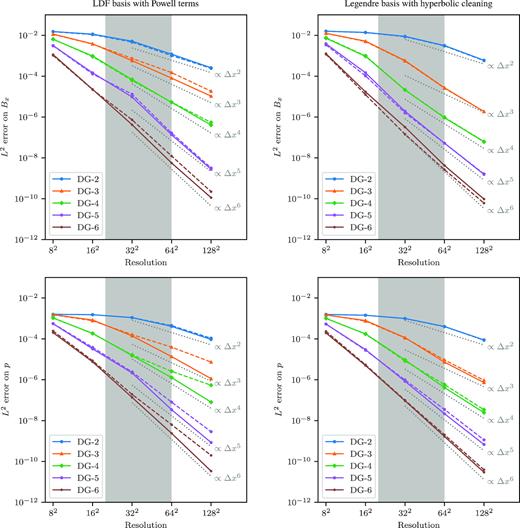
Convergence of errors in the MHD isodensity vortex problem. Solution L2 errors are plotted for Bx (top row) and pressure (bottom row), for both the LDF basis with Powell terms (left-hand column), and Legendre basis with hyperbolic cleaning (right-hand column). Errors are measured at time t = 20 after the vortex has crossed the whole computational domain. Dotted lines show theoretical slopes for convergence orders 2–6. Solid and dashed lines correspond to errors for an advection angle α = 45° and 30°, respectively. With the Legendre basis, the errors are insensitive to the vortex advection angle. With the LDF basis, the effective convergence order generally degrades slightly with α = 30°, in particular for the pressure. The shaded area corresponds to a range of resolutions for which the vortex is resolved but not over-resolved (see discussion in the text).

Figure 4.

Convergence of errors in the MHD isodensity vortex problem. Solution L² errors are plotted for B_x (top row) and pressure (bottom row), for both the LDF basis with Powell terms (left-hand column), and Legendre basis with hyperbolic cleaning (right-hand column). Errors are measured at time t = 20 after the vortex has crossed the whole computational domain. Dotted lines show theoretical slopes for convergence orders 2–6. Solid and dashed lines correspond to errors for an advection angle α = 45° and 30°, respectively. With the Legendre basis, the errors are insensitive to the vortex advection angle. With the LDF basis, the effective convergence order generally degrades slightly with α = 30°, in particular for the pressure. The shaded area corresponds to a range of resolutions for which the vortex is resolved but not over-resolved (see discussion in the text).

Open in new tab Download slide

We find that the code achieves the expected convergence order overall. When using LDF basis functions however, the effective order of convergence is degraded with α = 30° in the case of over-resolved solutions. This effect is mostly visible on the pressure, in the lower left panel of Fig. 4. We speculate that this effect is caused by some instability related to the LDF bases, whose discussion we postpone to the end of this section.

We first comment on the evolution of the global numerical divergence present in the solution as a function of scheme order and grid resolution. Fig. 5 presents the norm of the magnetic field divergence for the smooth vortex problem at final time t = 20, for both the Powell and hyperbolic cleaning schemes. The norm of the divergence is computed using equation (C2), which is sensitive to the divergence inside the cells, as well as to discontinuities of the normal component of |$\boldsymbol B$| across cell faces. We find that the divergence asymptotically converges to zero with resolution for the higher orders, however, the convergence order of |${\nabla }{\cdot }{\boldsymbol B}$| is generally slower than scheme order: for the cleaning scheme, the effective order of convergence is about one order less than the spatial order of the scheme – as one would expect for a first derivative of a field. For the Powell scheme, the convergence rate suffers some additional degradation, and presents a dependence on the angle α similar to the pressure errors of Fig. 4. In addition, the convergence of |${\nabla }{\cdot }{\boldsymbol B}$| is very sensitive to the resolved character of the solution for this smooth problem. For resolved smooth solutions (right of the grey band in Fig. 5), higher order schemes provide a more accurate representation of the solution, thereby reducing the discontinuity of the normal component of the magnetic field and allowing the global divergence of |$\boldsymbol B$| to converge to zero with order and resolution. For unresolved solutions on the other hand (left of the grey band in Fig. 5), additional resolution does not translate into reduction of the divergence, particularly at low scheme orders. For the adopted stringent definition of |$\left\Vert {\nabla }{\cdot }{\boldsymbol B}\right\Vert _1$| given by equation (C2), the Powell convergence rates for |${\nabla }{\cdot }{\boldsymbol B}$| are generally slightly slower than with hyperbolic cleaning on this problem. Interestingly, we found that the norm of the more lenient ‘signed divergence’ definition of equation (C4) asymptotically converges, for both Powell and cleaning methods, at a rate matching the spatial order of the scheme.

$Convergence of ${\nabla }{\cdot }{\boldsymbol B}$ in the MHD isodensity vortex problem. The norm of the divergence of the magnetic field (defined as in equation C2) is shown at t = 20 for the LDF basis with Powell terms (left-hand panel), and Legendre basis with hyperbolic cleaning (right-hand panel). Similarly to Fig. 4, dotted lines show theoretical slopes for convergence orders 2–6, solid and dashed lines correspond to α = 45° and 30°, respectively, and the shaded area corresponds to a range of resolutions for which the vortex is barely resolved.$

Figure 5.

Convergence of |${\nabla }{\cdot }{\boldsymbol B}$| in the MHD isodensity vortex problem. The norm of the divergence of the magnetic field (defined as in equation C2) is shown at t = 20 for the LDF basis with Powell terms (left-hand panel), and Legendre basis with hyperbolic cleaning (right-hand panel). Similarly to Fig. 4, dotted lines show theoretical slopes for convergence orders 2–6, solid and dashed lines correspond to α = 45° and 30°, respectively, and the shaded area corresponds to a range of resolutions for which the vortex is barely resolved.

Open in new tab Download slide

We now discuss the convergence order degradation observed with the Powell scheme. It is tempting to point at the lack of divergence damping with the Powell scheme as a possible culprit, because for such schemes, divergence errors are known not to converge away with resolution for discontinuous solutions (Tóth 2000). Dumbser et al. (2008) also suggested that high-order methods alone are not enough to achieve optimal convergence without some form of divergence cleaning. However, we found that a similar convergence degradation also appears when using hyperbolic cleaning on top of LDF bases – whereas hyperbolic cleaning with Legendre bases is immune, as Fig. 4 demonstrates. This suggests that the effect could be connected to the LDF bases, rather than caused by the Powell treatment alone.

We suspect that this deterioration is caused by the joint use of LDF basis functions, together with the continuous treatment of the normal component of |$\boldsymbol B$| in the chosen HLLD Riemann solver. While the detailed mechanics of this effect remain unclear at this point, we speculate that projection of source terms (in particular at the faces) on to LDF bases could in some cases contaminate high-order modes (see Appendix B). Potential ways to alleviate this issue with HLLD fluxes could be to rely on an eight-wave version of this Riemann solver, for example the one developed by Fuchs et al. (2011), or to combine different flux functions based on local smoothness of the solution (see e.g. Derigs et al. 2016). We leave these investigations to future work.

At this point, we also wish to stress that this convergence order degradation does not appear to be of great practical importance at this stage, because the errors are still well behaved and the beneficial effects of order convergence are still present, especially in the shaded area where the problem is marginally resolved: at resolutions around 32², order convergence helps capture the vortex much more efficiently than spatial convergence, with both choices of divergence control. It is of course possible that this effect is only the early-time manifestation of a more serious long-term instability, however we have seen no indication of such problems in our test runs so far. We believe these results demonstrate the necessity and value of testing multidimensional schemes in non-grid-aligned configurations (i.e. α = 30° in this case).

5.2.3 Circularly polarized Alfvén wave problem in 2D

Circularly polarized Alfvén waves are simple, exact smooth analytic solutions of the MHD equations for any wave perturbation amplitude. They are therefore particularly suitable to study the convergence order of the scheme, as well as its amount of numerical dispersion and dissipation. They consist of plane waves in which the magnetic field and velocity oscillate in phase in a circular polarization perpendicular to the propagation direction.

We broadly follow the travelling wave set-up proposed by Tóth (2000). Using periodic boundary conditions on a square domain [0, L]², we construct an Alfvén plane wave of unit wavelength, propagating at angle α > 0 with the x-axis. In order to respect periodicity, we pick α and L such that the box extends for exactly one wavelength in the y-direction, and m wavelengths in the x-direction (with m > 0 an integer). This implies |$\alpha = \arctan (1/m)$| and L = 1/sin α. We pick m = 2 which yields α ≈ 26.6°, L ≈ 2.24. This ensures that the problem is truly 2D. Calling |$(\parallel, \perp, z)$| the rotated (x, y, z) frame so that the wave propagates along the |$\parallel$| direction, the phase of the wave at any point (x, y) is given by |$\phi = 2 \pi x_\parallel$|⁠, with |$x_\parallel = x \cos \alpha + y \sin \alpha$|⁠. The magnetic field is initialized as |$(B_\parallel, B_\perp, B_z) = (1, \epsilon \sin \phi, \epsilon \cos \phi)$|⁠, and the initial velocity is set to |$(v_\parallel, v_\perp, v_z) = (v_0, \epsilon \sin \phi, \epsilon \cos \phi)$|⁠. We set |$\epsilon = 0.1$| and take v₀ = 0, which produces waves travelling along the |$\parallel$| direction towards negative |$x_\parallel$| at the Alfvén velocity |$v_\mathrm{ A} = B_\parallel / \sqrt{\rho } = 1$|⁠. Density and pressure are uniform with ρ = 1, p = 0.1, and we take γ = 5/3. Note that the magnetic pressure is uniform thanks to the |$B_\parallel$| and |$B_\perp$| components being in quadrature, and exact pressure equilibrium is achieved.

The analytic solution to this problem at any time t for the complete state vector |$\boldsymbol u$| is simply |$\boldsymbol u(x,y,t) = \boldsymbol u_0(x - (v_0-v_\mathrm{ A}) t \cos \alpha , y - (v_0-v_\mathrm{ A}) t \sin \alpha)$|⁠, where the signs of −v_A reflect the fact that the wave travels towards negative |$x_\parallel$|⁠.

Unfortunately, although it is an exact solution of non-linear MHD, this set-up is subject to parametric instabilities, which are easily triggered by low dissipation high-order schemes (see e.g. the discussion in Balsara et al. 2009, and references therein). In practice, this restricts convergence order tests to low resolutions, before the instability starts picking up and dominating the very low errors of high-order schemes. We present results with up to 64 grid points per dimension, which is comparable to the maximum resolution shown by Balsara et al. (2009).

Fig. 6 presents the L² solution errors for the x component of the magnetic field, after the wave has crossed one wavelength at time t = 1. The convergence order generally follows the theoretical order of convergence for both divergence control schemes. Note that at 64² resolution, the error of the fifth-order scheme starts levelling off at around 10⁻⁸, which we attribute to the triggering of the aforementioned parametric instability; Balsara et al. (2009) found evidence for this effect in their fourth-order code at comparable resolutions in their 3D Alfvén wave problem. Note also that our Powell scheme – which relies on LDF bases – suffers from a slightly degraded convergence rate for the fourth-order DG-4 scheme compared to hyperbolic cleaning. We deem that this effect could be related to the observed deterioration of the convergence order for the isodensity MHD vortex of Section 5.2.2.

Convergence of errors in the 2D Alfvén wave problem. Solution L2 errors on the x component of the magnetic field are shown for the LDF basis with Powell terms (left), and Legendre basis with hyperbolic cleaning (right). Errors are computed after the wave has crossed five wavelengths, at time t = 5. At the lowest resolutions, the DG-2 and DG-3 schemes do not accurately capture the wavefronts, which explains their apparent superconvergence. At error levels ∼10−8, the solution is polluted by the parametric instability of Alfvén waves discussed in the text. The effective order of convergence is degraded for the DG-4 scheme with LDF bases, probably because of projection effects. We refer to the text for a discussion of these last two effects.

Figure 6.

Convergence of errors in the 2D Alfvén wave problem. Solution L² errors on the x component of the magnetic field are shown for the LDF basis with Powell terms (left), and Legendre basis with hyperbolic cleaning (right). Errors are computed after the wave has crossed five wavelengths, at time t = 5. At the lowest resolutions, the DG-2 and DG-3 schemes do not accurately capture the wavefronts, which explains their apparent superconvergence. At error levels ∼10⁻⁸, the solution is polluted by the parametric instability of Alfvén waves discussed in the text. The effective order of convergence is degraded for the DG-4 scheme with LDF bases, probably because of projection effects. We refer to the text for a discussion of these last two effects.

Open in new tab Download slide

5.2.4 Circularly polarized Alfvén wave problem in 3D

To test convergence order of the code in 3D, we run a comparable Alfvén wave set-up, partially based on Balsara et al. (2009). For this problem, the domain is [0, 1]³ with periodic boundary conditions in all three directions. We take a uniform background density ρ = 1 and thermal pressure p = 100.

A rotated coordinate system |$(x', y', z')$| is set-up so that the |$x'$|-direction is aligned with the cube diagonal, following the exact transformation described in Balsara et al. (2009). Letting ϕ be the phase angle of the wave, the velocity field in the primed reference frame is |$\boldsymbol v^{\prime } = (1, \epsilon \cos \phi , \epsilon \sin \phi)$|⁠, while the magnetic field is |$\boldsymbol B^{\prime } = (1, -\epsilon \cos \phi , -\epsilon \sin \phi)$|⁠, for which we pick |$\epsilon = 0.02$|⁠. The unprimed velocity and magnetic fields are obtained by transforming back to unprimed coordinates.

The resulting wave travels at speed 2 along |$x'$|⁠, since it has Alfvén velocity 1 and is also advected with the flow with velocity 1 along |$x'$|due to our choice of |$\boldsymbol v^{\prime }$|⁠. The phase angle ϕ is therefore given by:

\begin{eqnarray*} \phi = \frac{2\pi }{\lambda } (x^{\prime } - 2t). \end{eqnarray*}

(62)

Choosing the wavelength |$\lambda = 1/\sqrt{3}$| ensures that the problem is periodic in all three directions x, y, and z, since whenever we cross one box length in one of these directions, |$x'$| shifts by |$1/\sqrt{3}$|⁠. With this choice of λ, the cube diagonal crosses three wave periods. The problem is run until time |$t_\mathrm{ f} = \sqrt{3}/2$|⁠, after which the three wavefronts will have crossed the whole domain once.

Fig. 7 shows the convergence of the errors on the |$\boldsymbol B_\mathrm{ x}$| component with the Powell and hyperbolic cleaning schemes for scheme orders 2–4. Both schemes follow overall the expected order of convergence.

$Convergence of errors in the 3D Alfvén wave problem. Solution L2 errors on the x component of the magnetic field are shown for the LDF basis with Powell terms (left), and Legendre basis with hyperbolic cleaning (right). Errors are computed after three wavefronts have crossed the box domain, at time $t_\mathrm{ f} = \sqrt{3}/2$.$

Figure 7.

Convergence of errors in the 3D Alfvén wave problem. Solution L² errors on the x component of the magnetic field are shown for the LDF basis with Powell terms (left), and Legendre basis with hyperbolic cleaning (right). Errors are computed after three wavefronts have crossed the box domain, at time |$t_\mathrm{ f} = \sqrt{3}/2$|⁠.

Open in new tab Download slide

5.3 Shock problems

We now turn to test problems in 1D, 2D, and 3D designed to test the shock capturing properties of the scheme.

5.3.1 Brio–Wu shock tube

The famous shock tube problem introduced by Brio & Wu (1988) has now become a classic of shock tests for MHD codes. For this test, we take the computational domain to be [0, 1] with fixed boundary conditions at x = 0 and 1. In the whole domain, the flow is initially at rest (⁠|$\boldsymbol v=0$|⁠) and (B_x, B_{|$\mathrm{ z}$|}) = (0.75, 0). The initial primitive variables are discontinuous at x = 0.5, with the left and right states given by (ρ, p, B_y)_L = (1, 1, 1) and (ρ, p, B_y)_R = (0.125, 0.1, −1) respectively. We set γ = 2, and run the simulation until final time t_f = 0.1. Note that we actually run our 1D test problems in 2D, with perfectly y-independent initial conditions and periodic boundary conditions in y, in order to test the numerical stability of the 1D set-up. We check that no significant y dependence of the solution has developed at the final time.

Fig. 8 presents the density, pressure, and y component of the magnetic field in the Brio–Wu shock tube test problem at final time t_f = 0.1, using the third-order DG-3 scheme at resolution level ℓ = 9 (corresponding to 512 cells). The reference solution was obtained using athena (Stone et al. 2008) with the third-order Roe solver on 10⁴ mesh points. The DG-3 scheme captures all the MHD waves correctly, and the shocks are resolved with 1–2 cells, whereas the contact discontinuity is resolved within about four cells. The limiter is efficient at preventing overshoots around shocks, although some oscillations are visible around the contact discontinuity and after the right rarefaction wave, probably due to a rather lenient global limiter setting used across all of our tests. A more finely tuned or more sophisticated limiter could help reducing these oscillations. We note however that we observed identical oscillations of similar amplitude and wavelength with athena with HLLD and third-order reconstruction at the same resolution of 512 cells.

Figure 8.

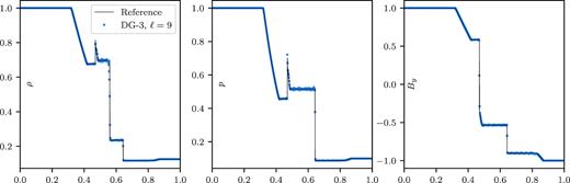
Brio–Wu MHD shock tube problem. The density, pressure, and y component of the magnetic field are shown at t = 0.1 for a grid with 512 cells (resolution level ℓ = 9). The reference solution was computed using athena with the third-order Roe solver on 10⁴ mesh points. All the MHD waves are correctly captured and shocks are captured within 1–2 cells without overshooting. Some oscillations are visible, probably due to the simple limiting procedure employed (see the text).

Open in new tab Download slide

5.3.2 1D MHD Shu–Osher test problem

The so-called hydrodynamical Shu–Osher test problem, introduced by Shu & Osher (1989), follows the interaction of a supersonic shockwave with smooth density perturbations. It tests the scheme’s ability to resolve small-scale features in the presence of strong shocks. An MHD version of the test was proposed by Susanto (2014), and used in particular by Derigs et al. (2016) to test their MHD scheme in flash. We follow the set-up of these two papers. The computational domain is [−5, 5] with reflective boundary conditions. At t = 0, the shock interface is located at x₀ = −4. In the region x ≤ x₀, a smooth supersonic flow is initialized with primitive state given by |$(\rho , \boldsymbol v_\mathrm{ x}, \boldsymbol v_\mathrm{ y}, \boldsymbol v_\mathrm{ z}, p, \boldsymbol B_\mathrm{ x}, \boldsymbol B_\mathrm{ y}, \boldsymbol B_\mathrm{ z}) = (3.5, 5.8846, 1.1198, 0, 42.0267, 1, 3.6359, 0)$|⁠. In the rest of the domain x > x₀, smooth stationary perturbations are set-up with primitive state (1 + 0.2sin 5x, 0, 0, 0, 1, 1, 1, 0). The flow is evolved until final time t_f = 0.7.

The density profile at t_f is shown in Fig. 9, for resolution levels 7 (128 cells) and 8 (256 cells). To compare the results and focus on the impact of the spatial discretization order, we use the RK3 SSP time integrator for all runs of this test problem, but we have checked that the results are unchanged if we use RK2 for the DG-2 schemes. The zoom-in panel on the right shows that going from second to third order greatly improves the capturing of the strong oscillations in the interaction region, in particular at the lower resolution level 7. This test problem demonstrates the ability of higher order methods to capture finer features in the flow with lower numerical diffusion. In particular, our third-order scheme is very competitive for this test problem: Chakravarthy, Arora & Chakraborty (2015) show that they can capture the oscillations with 400 grid points (about 14 points per oscillation period, see their fig. 9), Derigs et al. (2016) demonstrate good capturing with 256 points (about 9 per period, see their fig. 6), and with the DG-3 scheme, we obtain results comparable to this latter work with only 128 total grid points (i.e. 4–5 points per period, see the corresponding DG-3 ℓ = 7 line in Fig. 9).

Figure 9.

MHD Shu–Osher shock tube test problem. The density profile is shown at final time t_f = 0.7. This figure can be directly compared to Derigs et al. (2016). The reference solution was computed using athena with the third-order Roe solver on 10⁴ mesh points. The right-hand panel is a zoom on the region shown framed in the left-hand panel. The numerical solution for second-order (DG-2) and third-order (DG-3) schemes are shown, for resolution levels ℓ = 7 (128 grid points) and ℓ = 8 (256 points).

Open in new tab Download slide

5.3.3 Orszag–Tang vortex problem

We now consider the Orszag–Tang vortex problem, a widely-used test problem for MHD. The vortex starts from a smooth initial field configuration, and quickly forms shocks before transitioning to 2D MHD turbulence.

For this problem, our computational domain is [0, 1]² and we use γ = 5/3. The initial density and pressure are uniform, with |$\rho = \frac{25}{36\pi }$| and |$p= \frac{5}{12\pi }$|⁠. The initial gas velocity field is |$\boldsymbol v= (-\sin (2\pi y), \sin (2\pi x), 0)$|⁠, and the initial magnetic field is |$\boldsymbol B= (-B_0 \sin (2\pi y), B_0 \sin (4\pi x), 0)$|⁠, with |$B_0 = 1/\sqrt{4\pi }$|⁠.

The solution at t = 0.5 is presented in Fig. 10. This is the well-recognizable picture of the Orszag–Tang vortex, presented by many authors discussing MHD codes. Note that we obtain both sharp shocks and smooth, noise-free flow with resolved features between the shocks. During our experiments, we found that details of both the limiting procedure and the Powell term discretization could strongly impact the shape of the low-density smooth regions.

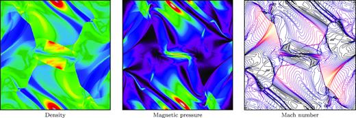
Orszag–Tang vortex test problem at t = 0.5. The density, pressure, and Mach number are shown on a 5122 grid, computed using the third-order DG scheme with the Powell method.

Figure 10.

Orszag–Tang vortex test problem at t = 0.5. The density, pressure, and Mach number are shown on a 512² grid, computed using the third-order DG scheme with the Powell method.

Open in new tab Download slide

While the Orszag–Tang vortex is a classic MHD test, many authors do not discuss how their codes capture the evolution beyond t = 0.5. During our experiments, we found that while many limiters and Powell term prescriptions work equivalently well until t = 0.5, long time integration of this problem can be challenging, in particular for divergence errors, as noted by Balsara (1998). We found that running the problem for longer times could discriminate well between otherwise seemingly equivalent discretizations. In particular, at times t ∈ [0.75, 0.85], complex shock interactions occur near the centre of the box which can easily cause divergence blow-ups. In Fig. 11, we show maps of the magnetic pressure at t = 1 with both divergence control methods at level 8 resolution, and for the Powell method at level 9 resolution. While some differences can be we observed in the central vortex and in the finer detailed structure of the folds, the resulting magnetic field configurations are in good agreement, even well into the transition into 2D turbulence.

Figure 11.

Orszag–Tang vortex test problem at t = 1. The magnetic pressure is shown for the third-order DG scheme with the Powell and divergence cleaning methods on a 256² grid (left and centre, respectively), and for the Powell method on a 512² grid (right). All resulting magnetic field configurations are in good agreement.

Open in new tab Download slide

Fig. 12 shows maps of the normalized divergence using the DG-3 Powell and cleaning schemes at 512² resolution, as defined in Appendix C2. The divergence is concentrated around shocks, with both methods forming similar patterns. Because hyperbolic cleaning propagates the divergence through the simulation box, divergence waves quickly fill the whole domain, producing the fairly uniform background clearly visible in the centre panel. The right-hand panel of Fig. 12 presents the time evolution of the divergence with both methods up to t = 5, demonstrating that |${\nabla }{\cdot }{\boldsymbol B}$| remains under control for long run times with both schemes. The Powell method results in divergence levels about one order of magnitude greater than hyperbolic cleaning, in broad overall agreement with existing comparisons across different test problems (see e.g. Tricco & Price 2012; Hopkins & Raives 2016; Derigs et al. 2018).

Figure 12.

Magnetic field divergence in the Orszag–Tang test problem. Maps of the normalized magnetic field divergence (see Appendix C2) are shown for the DG-3 scheme at 512² resolution using the Powell (left) and divergence cleaning (centre) schemes. The right-hand panel shows the time evolution of the L¹ norm of the magnetic field divergence for both methods.

Open in new tab Download slide

Because the Orszag–Tang test gives rise to many complex flow features including regions of potentially severe numerical divergence, we also use this test problem to assess the impact of non-conservative Powell terms on scheme conservation. We find that in general the total energy is the conserved quantity most directly impacted by the Powell term. Fig. 13 shows the time evolution of the magnetic, kinetic, thermal, and total energies (E_mag, E_kin, E_th, and E_tot respectively) for the DG-3 scheme over 0 ≤ t ≤ 1. In the bottom panel, the energies are shown for resolution levels ℓ = 7 (128²) and ℓ = 9 (512²) and for both divergence control schemes. The energy histories are in good overall agreement across methods and resolutions, although differences develop over time. The top panel shows the slight deviation of the total energy E_tot from its initial value due to non-conservative source terms with the Powell scheme. Over the whole time evolution, E_tot has deviated by at most |$0.6{{\ \rm per\ cent}}$| for ℓ = 7, and |$0.3{{\ \rm per\ cent}}$| for ℓ = 9. Increasing the resolution seems to contribute to reduce the deviation of E_tot, even though it is known that divergence errors in general do not locally converge away with resolution (Tóth 2000). Note that the deviation is not evolving monotonically, as such, it is difficult to appreciate the long-term impact of non-conservative source terms on the solution. Note also that the effect of the divergence control scheme on the magnetic energy (lower inset) is comparable in magnitude to the effect of resolution, so the detailed differences in energies may not all be attributed to the difference in divergence treatment.

Evolution of energies in the Orszag–Tang vortex problem, for the third-order DG-3 scheme, at resolution levels 7 (1282) and 9 (5122) using the Powell and hyperbolic cleaning schemes. The bottom panel shows the time evolution of the different energies integrated over the whole domain, while the top panel shows the deviation in the total energy Etot from its initial value due to non-conservative terms for the Powell scheme.

Figure 13.

Evolution of energies in the Orszag–Tang vortex problem, for the third-order DG-3 scheme, at resolution levels 7 (128²) and 9 (512²) using the Powell and hyperbolic cleaning schemes. The bottom panel shows the time evolution of the different energies integrated over the whole domain, while the top panel shows the deviation in the total energy E_tot from its initial value due to non-conservative terms for the Powell scheme.

Open in new tab Download slide

We point out that total conservation is not a sufficient test of the quality of the solution against divergence errors, because energy can be created and destroyed locally in the flow with different signs, depending on the sign of various quantities in the source term (29). While the conservation results are encouraging overall, we intend to perform more careful comparisons when applying both schemes to physical problems. Driven turbulence problems in particular may turn out to be more sensitive to non-conservation issues, because energy is continually injected in the simulation domain.

We conclude this section with Fig. 14, which shows the same Orszag–Tang problem run up to t = 0.5 with adaptive resolution from 64² to 512², using the DG-3 Powell and divergence cleaning schemes. The solution may be directly compared to the 512² Cartesian run of Fig. 10. The AMR solutions obtained using both divergence control methods are very similar, and both in very good agreement with the Cartesian solution. On the Powell density map, some slight ripple-like noise is visible in a few localized smooth regions in the vicinity of shocks. This is likely the result of the interaction of the divergence control method with AMR, as those features are absent from both the Cartesian Powell and AMR divergence cleaning runs.

Orszag–Tang vortex problem with AMR at t = 0.5, from resolution levels 6–9 (642–5122) using the DG-3 Powell (top) and divergence cleaning (bottom) schemes. The columns show the density field (left), the geometry of the AMR grid (centre), and the normalized magnetic field divergence (right). The refinement is based on the density and magnetic field components. The density map may be directly compared to the 5122 Cartesian run of Fig 10.

Figure 14.

Orszag–Tang vortex problem with AMR at t = 0.5, from resolution levels 6–9 (64²–512²) using the DG-3 Powell (top) and divergence cleaning (bottom) schemes. The columns show the density field (left), the geometry of the AMR grid (centre), and the normalized magnetic field divergence (right). The refinement is based on the density and magnetic field components. The density map may be directly compared to the 512² Cartesian run of Fig 10.

Open in new tab Download slide

The adaptive mesh provides both memory and wall time reduction for this problem. With the Powell scheme, at t = 0.5, the AMR grid of Fig. 14 features 2.4 times fewer cells than the 512² Cartesian grid of Fig. 10 of equivalent maximum resolution. The same AMR run also reaches t = 0.5 about 3.0 times faster: in addition to requiring fewer cells, the adaptive mesh allows computing the early stages of the evolution with a larger time-step, because the initial Orszag–Tang flow is very smooth and therefore well captured everywhere by coarse cells.

5.3.4 Advected Orszag–Tang vortex

In this problem, we test the code’s Galilean invariance by running the Orszag–Tang vortex test case up to t_f = 0.5, giving the fluid an additional uniform global bulk velocity |$\boldsymbol v_0 = (10, 10, 0)$|⁠. This corresponds to a hypersonic advection with initial Mach number ≈14. At time t_f, the flow will have crossed the box five times in the x- and y-directions, and end up in a configuration identical to the non-advected problem at the same time.

We present the results for advected and non-advected problems for second-order DG-2 and third-order DG-3 in Fig. 15. For this test, all runs use the same RK3 SSP time integrator. Comparing the density contours of the non-advected and advected DG-2 solutions at resolution 128² (first row), we notice that the supersonic bulk advection velocity increases numerical diffusion significantly. In the advected solution, the shocks are smoothed out, the density valleys are shallower, and some of the complex structures, e.g. in the lower right corner of the domain, are eroded. This diffusion is clearly visible on the difference map on the right-hand column, which shows the deviation between the advected and the non-advected maps, together with the L² norm of the difference. For each run configuration, the total number of degrees of freedom N_DoF is indicated at the left of the corresponding row.

Figure 15.

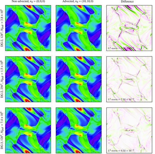
Advected Orszag–Tang vortex problem. We show the density cell averages at t = 0.5 for the non-advected Orszag–Tang vortex problem (left-hand column), the advected problem (centre column), and the difference between the two (right-hand column), for various combinations of scheme order and resolutions (rows). The top row is run using second-order DG at 128², the middle row increases the resolution of the second-order method to 256², while the bottom row uses the third-order scheme at the lower 128² resolution. The colour scales are identical across all density maps and all difference maps. In the row labels, N_DoF describes the total number of scalar degrees of freedom in the problem. This test shows the ability of higher order methods to reduce advection errors and preserve finer structures in the flow, even with limiting in the presence of MHD shocks, at a smaller cost in terms of degrees of freedom.

Open in new tab Download slide

The middle row of Fig. 15 shows the same second-order scheme, this time with a spatial resolution of 256². This increased resolution results in four times as many degrees of freedom, and is able to significantly improve the advection errors in smooth regions of the flow. However, the L² norm of the advection error is only reduced by a factor of about 1.8, at the cost of a four times increase in the number of degrees of freedom, and eight times increase in the time-to-solution due to the CFL condition.

In the bottom row, the resolution was taken back to 128², but the order was increased to DG-3. Compared to DG-2 at the same resolution, this represents only a 1.95 times increase in the number of degrees of freedom, and a measured 3.2 times increase in the time-to-solution. With the third-order algorithm, advection errors in smooth regions of the flow are almost completely eliminated, and errors are also reduced close to shocks, resulting in the lowest L² error norm and best overall preservation of Galilean invariance across the three runs.

This test shows that the reduction of advection errors offered by higher orders, which was discussed by e.g. Robertson et al. (2010) and demonstrated with DG by Schaal et al. (2015) for Euler hydrodynamics problems, carries over to complex MHD flows in presence of shocks, even with our relatively simple slope limiting prescription. It also shows that in some cases, increasing the order can result in notable improvements, and at a lesser expense in terms of degrees of freedom than increasing the resolution: in this case, DG-3 128² requires only about half as many degrees of freedom as DG-2 256², runs more than twice as fast, and results in smaller errors.

5.3.5 MHD rotor problem

We now look at the so-called 2D MHD rotor problem introduced by Balsara & Spicer (1999b), for which we use the more stringent ‘first rotor problem’ variant of Tóth (2000). In this set-up, a dense disc of fluid rotates within a static fluid background, with a gradual velocity tapering layer between the disc edge and the ambient fluid. An initially uniform magnetic field is present, which winds up with the disc rotation and contains the dense rotating region through magnetic field tension. The computational domain is [0, 1]². Initial pressure and magnetic fields are uniform in the whole domain, with p = 1 and |$\boldsymbol B= (5/\sqrt{4\pi }, 0, 0)$|⁠. The central rotating disc is defined by r < r₀ where r² = (x − 0.5)² + (y − 0.5)², and r₀ = 0.1. Inside the disc, ρ = 10, and the disc rotates rigidly with |$(\boldsymbol v_\mathrm{ x}, \boldsymbol v_\mathrm{ y}) = (0.5-y, x-0.5)v_0/r_0$| with v₀ = 2. Beyond r > r₁ lies the background fluid, which has density ρ = 1 and is at rest: |$\boldsymbol v_\mathrm{ x} = \boldsymbol v_\mathrm{ y} = 0$|⁠. In the annulus r₀ ≤ r ≤ r₁ = 0.115, the taper region linearly interpolates between the disc and the background, with |$(\boldsymbol v_\mathrm{ x}, \boldsymbol v_\mathrm{ y}) = (0.5-y, x-0.5) v_0 f / r_0$| and ρ = 1 + 9f, where f = (r₁ − r)/(r₁ − r₀) is the tapering function. The simulation runs until t_f = 0.15. We use periodic boundary conditions, but note that the perturbations will not have reached the domain boundaries at t_f, so reflective or inflow boundary conditions are also suitable.

The density, magnetic pressure, and Mach number contours are presented in Fig. 16 for the Powell scheme. We note that the central contours show a very good conservation of the circular rotation pattern, which was found by Tóth (2000) to be challenging for some MHD schemes. Also, there are no distortions at the outskirts of the central almond-shaped disc region, which suggests that the magnetic field divergence is well controlled (see Li & Shu 2005). Fig. 17 presents slices² of the magnetic field at t_f across horizontal and vertical cuts through the centre of the box, and can be compared to fig. 26 of Stone et al. (2008) with which they show good agreement.

Magnetic rotor test problem. The density, pressure, and Mach number contours in the 2D magnetic adiabatic rotor test are shown, on a 5122 grid using the third-order Powell scheme.

Figure 16.

Magnetic rotor test problem. The density, pressure, and Mach number contours in the 2D magnetic adiabatic rotor test are shown, on a 512² grid using the third-order Powell scheme.

Open in new tab Download slide

Figure 17.

Slices of the magnetic field in the MHD rotor test, along y = 0.5 (top) and x = 0.5 (bottom), computed using DG-3 with Powell terms. The slices can be compared to Stone et al. (2008).

Open in new tab Download slide

Finally, Fig. 18 shows maps of the normalized magnetic field divergence for the Powell and cleaning schemes. Similarly to the case of the Orszag–Tang vortex presented in Fig. 12, |${\nabla }{\cdot }{\boldsymbol B}$| is mostly concentrated in regions around shocks. Hyperbolic cleaning propagates the divergence faster than MHD waves, creating ripples in the magnetic field which propagate away from the centre in the background fluid. The time evolution of the divergence is also shown on the right-hand panel; both the Powell and cleaning schemes follow a very similar overall time evolution.

Magnetic field divergence in the rotor test problem. Maps of the normalized magnetic field divergence are shown for the DG-3 scheme at 5122 resolution using the Powell (left) and divergence cleaning (centre) schemes. The right-hand panel shows the time evolution of the L1 norm of the magnetic field divergence for both methods.

Figure 18.

Magnetic field divergence in the rotor test problem. Maps of the normalized magnetic field divergence are shown for the DG-3 scheme at 512² resolution using the Powell (left) and divergence cleaning (centre) schemes. The right-hand panel shows the time evolution of the L¹ norm of the magnetic field divergence for both methods.

Open in new tab Download slide

In Fig. 19, we show the MHD rotor problem with AMR (64²–512²), using the DG-3 Powell and divergence cleaning schemes. Here again, the solution may be directly compared to the 512² Cartesian run of Fig. 16, and like for the Orszag–Tang vortex, we find that the AMR solutions are in very good agreement with each other, as well as with the Cartesian solution. This solution can also be compared to figures 6 and 7 from Derigs et al. (2018), which also display an AMR solution for this problem spanning the same resolution range. Their ‘no GLM’ method is a Powell-type method (extra source terms, no divergence cleaning), which produces divergence artefacts (see their fig. 7); we observe no such damage in our Powell solution.

MHD rotor problem with AMR at t = 0.15, from resolution levels 6–9 (642–5122) using the DG-3 Powell (top) and divergence cleaning (bottom) schemes. The columns show the density field (left), the geometry of the AMR grid (centre), and the normalized magnetic field divergence (right). The refinement is based on the density and magnetic field components. The density map may be directly compared to the 5122 Cartesian run of Fig 16.

Figure 19.

MHD rotor problem with AMR at t = 0.15, from resolution levels 6–9 (64²–512²) using the DG-3 Powell (top) and divergence cleaning (bottom) schemes. The columns show the density field (left), the geometry of the AMR grid (centre), and the normalized magnetic field divergence (right). The refinement is based on the density and magnetic field components. The density map may be directly compared to the 512² Cartesian run of Fig 16.

Open in new tab Download slide

On this problem, we also see memory and time-to-solution gains with AMR. With the Powell scheme, at t = 0.15, the AMR rotor grid of Fig. 19 features 3.5 times fewer cells than the 512² Cartesian grid of equivalent maximum resolution of Fig. 16. That same point in time is reached 3.4 times faster with the AMR simulation compared to the Cartesian mesh, illustrating the important performance gains and memory savings that AMR can bring about already in 2D.

5.3.6 MHD blast wave in 2D

This test follows the evolution of MHD discontinuities in a strongly magnetized configuration. For this test, we adapt the version of Stone et al. (2008) to a square periodic domain [0, 1]². The background fluid has zero velocity, ρ = 1, p = 0.1, and magnetic field |$\boldsymbol B_0 = (B_0 \cos \alpha , B_0 \sin \alpha , 0)$| with B₀ = 1 and α = 45°. Within a radius r₀ = 0.1 of the centre of the box, we set p = 10, keeping all other primitive variables at their background values. We use γ = 5/3, and choose α = 45°. The simulation is run until a final time of t_f = 0.2.

Note that when running this test with |$\boldsymbol B_0$| aligned with the grid with our scheme, small localized finger-like features develop at the shock front around the axis of symmetry parallel to |$\boldsymbol B_0$|⁠, which we attribute to the so-called ‘carbuncle’ instability (Robinet et al. 2000). This instability manifests itself in the case of strong shocks exactly aligned with the grid directions, when using non-diffusive Riemann solvers. In few highly specific simulation configurations where this problem may appear, it may be resolved by a modification of the numerical fluxes (see e.g. Robinet et al. 2000; Stone et al. 2008); however here we do not modify the scheme to counter this peculiar instability.

We also successfully run this test with B₀ = 10, with an initial plasma β of 2 × 10⁻², which demonstrates the robustness of our implementation in highly magnetized shock configurations. In all cases, we find that the symmetry of the problem is very well preserved, as can be seen on the Mach number contours in Fig. 20. The shocks are sharp, while post-shock regions remain smooth.

2D MHD blast test problem. The density, magnetic pressure, and Mach number contours are shown on a 2562 grid using the third-order Powell scheme.

Figure 20.

2D MHD blast test problem. The density, magnetic pressure, and Mach number contours are shown on a 256² grid using the third-order Powell scheme.

Open in new tab Download slide

To investigate the potential impact of the Powell method on magnetic field divergence on this test problem, we also plot slices of the magnetic field in Fig. 21 following Hopkins & Raives (2016). Unlike these authors, we find no evidence of errors in the components of the magnetic field with the Powell scheme for this test problem in our scheme.

Figure 21.

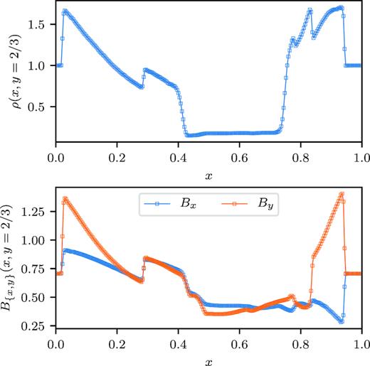
Slices across y = 2/3 in the MHD blast wave test problem, following Hopkins & Raives (2016), shown here for the DG-3 Powell scheme. We do not observe any of the dramatic errors noted by these authors on their tests with Powell terms.

Open in new tab Download slide

5.3.7 MHD blast wave in 3D

To test the shock-capturing and positivity preserving performance of the code in 3D, we adopt the 3D blast wave set-up of Balsara et al. (2009). The computation domain is [0, 1]³ with periodic boundary conditions. The background fluid is initially at rest with respect to the grid, with |$\boldsymbol v=0$|⁠, ρ = 1, and a uniform magnetic field |$\boldsymbol B= (B_0, B_0, B_0)$|⁠. To match the set-up for the slices presented in Balsara et al. (2009), we take |$B_0 = 100 \sqrt{3}^{-1} \sqrt{4\pi }^{-1}$| in our system of units.³ The pressure is set to p = 0.1 in the background, and within a central ball of radius r₀ = 0.1, we set p = 1000 to initialize the blast. This creates a near-infinite shock strength with a pressure ratio of 10⁴, in a strongly magnetized background with a plasma-β of 7.5 × 10⁻⁴. We take γ = 1.4, and run the simulation until final time t_f = 0.01.

Fig. 22 shows slices at constant z through the centre of the blast at t_f, for the third-order DG-3 method at resolution 128³. Note that for slicing purposes, care must be taken to place the blast centre exactly at the centre of a cell, which we achieve at 128³ resolution by shifting the centre of the high pressure ball by half a cell in every direction. The slices of Fig. 22 may be compared to fig. 11 in Balsara et al. (2009), which uses a higher resolution of 151³.

MHD blast wave in 3D. Slices in the (x, y) plane showing log density, magnitude of velocity, and magnitude of magnetic field at resolution 1283 with the third-order DG method.

Figure 22.

MHD blast wave in 3D. Slices in the (x, y) plane showing log density, magnitude of velocity, and magnitude of magnetic field at resolution 128³ with the third-order DG method.

Open in new tab Download slide

The DG Powell scheme is able to maintain positivity of the pressure and density in the whole domain, while finely capturing the very strong discontinuities and resolving the complex structures in the velocity. Note that no oscillations are visible around discontinuities. Some numerical noise is present in the post-shock regions for the density and pressure fields, but disappears with a more aggressive limiting threshold. This test shows the robustness and shock-capturing behaviour of the Powell scheme for 3D problems involving very strong magnetized shocks.

This problem proves particularly challenging for our implementation of hyperbolic cleaning. In such a low plasma-β set-up, changes in the magnetic field caused by hyperbolic cleaning propagate fast in the ambient medium at the cleaning speed c_h, and result in fluctuations of the magnetic pressure which locally cause negative thermal pressures far away and ahead of the MHD blast wavefront. These negative pressures are successfully but aggressively corrected by our positivity limiter, and although the computation does not crash, the gas temperature information is destroyed, which in turn damages the hydrodynamical solution in the background medium, far ahead of the fast MHD shocks (depending on the exact choice of c_h). Similar issues have been noted and worked on by a number of authors (e.g. Mignone & Tzeferacos 2010; Tricco & Price 2012; Susanto 2014; Tricco et al. 2016); we come back to this issue and possible solutions in the discussion.

5.4 Divergence control problems

We now turn to test problems more specifically aimed at evaluating the efficiency of the divergence control, with a focus on the Powell scheme. We have already discussed some aspects related to |${\nabla }{\cdot }{\boldsymbol B}$| in some of the previous test problems; we now show the stability of the Powell scheme and some consequences of its non-conservative source terms.

On a general note, like Balsara & Spicer (1999b), we found that problems with strong moving shocks, such as the blast or rotor problems, are not necessarily the most stringent tests of divergence control. Instead, colliding shocks whose convergence front is at rest with respect to the grid – such as the rotated shock tube of Tóth (2000) described in Section 5.4.3, or some shock–shock interactions in the Orszag–Tang vortex of Section 5.3.3 – proved to be much more challenging tests of the divergence control scheme and its stability in particular.

In addition to shock interactions, we found that smooth problems such as the simple advection of a magnetic field loop can also be unstable with inappropriate discretizations of the Powell term, and their smooth character makes it easier to follow the development of the divergence instability. Without Powell source terms, the instability usually grows faster with scheme order, as the numerical diffusion at lower orders helps slow down the divergence runaway.

5.4.1 Loop advection

This test follows the advection of a magnetic field loop after Gardiner & Stone (2005). On the periodic domain [−1, 1]², the background fluid has ρ = 1, p = 1, and a global advection velocity |$(\boldsymbol v_\mathrm{ x}, \boldsymbol v_\mathrm{ y}) = (2, 1)$| so that the ambient flow is not aligned with grid directions. Letting r be the radial distance to the centre of the box, the magnetic field is initialized from a vector potential |$\boldsymbol A = (0, 0, A_\mathrm{ z}(r))$| with |$\boldsymbol B= \nabla \times \boldsymbol A$|⁠. To define a magnetic field loop of radius r₀ = 0.3, we set A_{|$\mathrm{ z}$|}(r) = max (0, A₀(r₀ − r)). Taking A₀ = 10⁻³, we obtain a very weakly magnetized configuration with a plasma β of order 10⁶, in which the magnetic field is essentially a passive scalar. For this field configuration, the MHD current vanishes everywhere, except at r = 0, and r = r₀ where the corresponding current line and return current tube are singular.

The aim of the test is to verify that the current loop is advected without deformation or noise, and to monitor the time evolution and dissipation rate of the total magnetic energy, following Gardiner & Stone (2005) and Stone et al. (2008).

As discussed in Gardiner & Stone (2005), the linearized dynamics of the magnetic field involves the diagonal derivatives |$\partial \boldsymbol B_\mathrm{ x} / \partial x$|⁠, and this test is therefore sensitive to the |${\nabla }{\cdot }{\boldsymbol B}$| treatment, although this is mostly an issue for directionally split methods. In any case however, the linearized loop advection setup constitutes a so-called resonant hyperbolic problem, as discussed in Kemm (2013), and therefore constitutes a good test for the growth of divergence instabilities. We found this test to be particularly unstable without divergence control, even with a smooth non-singular loop configuration. Fig. 23 shows divergence maps for the loop advection problem for both the Powell and cleaning schemes, together with the time evolution of the divergence. With both schemes, the numerical divergence is well under control.

Figure 23.

Magnetic field divergence in the loop advection test problem. Maps of the non-normalized magnetic field divergence are shown for the DG-3 scheme at 128² resolution using the Powell (left) and divergence cleaning (centre) schemes. The right-hand panel shows the time evolution of the L¹ norm of the magnetic field divergence for both methods. Because the magnetic field vanishes outside of the loop, we do not normalize by the local magnetic field strength, and instead plot the absolute divergence in code units, given by equations (C1) and (C2) for the maps and time evolution, respectively.

Open in new tab Download slide

Fig. 24 shows the z component of the cell average of the current density |$\boldsymbol j = \nabla \times \boldsymbol B$| at final time t = 2 after two horizontal domain crossings, at resolution 128², for orders 2–4. For this comparison, we use the RK3 SSP time integrator across all spatial orders. The current density is a stringent diagnostic since, being a derivative of the magnetic field, it is very sensitive to noise and local fluctuations. The scheme preserves the exact circular shape of the current loop at all orders, with very little noise and oscillations in the current at all orders. In addition, the reduction in numerical diffusion and advection errors is clearly noticeable as order is increased. We also see that the current loop gets increasingly resolved at higher orders, showing an increase in effective resolution even for singular features.

$MHD current in the loop advection problem. The average z component of current density $\boldsymbol j = \nabla \times \boldsymbol B$ in each cell is shown for the Powell DG-2, DG-3, and DG-4 schemes at resolution 1282, at t = 2 after two horizontal domain crossings. The code preserves the shape of the current loop very well at all orders, and the test demonstrates the qualities or higher order schemes for reducing numerical diffusion.$

Figure 24.

MHD current in the loop advection problem. The average z component of current density |$\boldsymbol j = \nabla \times \boldsymbol B$| in each cell is shown for the Powell DG-2, DG-3, and DG-4 schemes at resolution 128², at t = 2 after two horizontal domain crossings. The code preserves the shape of the current loop very well at all orders, and the test demonstrates the qualities or higher order schemes for reducing numerical diffusion.

Open in new tab Download slide

The plot of Fig. 25 follows the time evolution of the normalized total magnetic energy during two horizontal domain crossings, at resolution 128². The results are shown for the Powell and hyperbolic cleaning schemes. The hyperbolic cleaning scheme seems slightly more diffusive, especially at lower orders. The corresponding decay time-scales may be fitted with the power-law functional form proposed in Gardiner & Stone (2005): E_mag(t) = A(1 − (t/τ)^α). For the Powell scheme, we measure τ ≈ 1.8 × 10⁴ for DG-2, τ ≈ 6.1 × 10⁷ for DG-3, and τ ≈ 6.0 × 10¹¹ for DG-4, which quantifies the strong reduction of the decay rate τ⁻¹ with increasing scheme order.

Time evolution of the magnetic energy in the field loop advection test, for the second-, third-, and fourth-order schemes, at resolution 1282. The solid lines correspond to the Powell scheme, whereas the dashed lines use hyperbolic divergence cleaning.

Figure 25.

Time evolution of the magnetic energy in the field loop advection test, for the second-, third-, and fourth-order schemes, at resolution 128². The solid lines correspond to the Powell scheme, whereas the dashed lines use hyperbolic divergence cleaning.

Open in new tab Download slide

5.4.2 Current sheet problem

A very stringent test of the capability of the code to handle numerical divergence and maintain positivity is the so-called current sheet problem (Hawley & Stone 1995; Gardiner & Stone 2005), which follows the evolution of sharp interfaces between regions with magnetic fields of opposing directions. The chosen fluid velocities will push and pull the interfaces along their normal direction, letting the magnetic tension act as a restoring force which results in Alfvén oscillations. At the interfaces – where the tangential component of the magnetic field flips sign – numerical reconnection will occur, forming growing isolated islands of reconnected magnetic regions. Similar configurations have also been used in the context of non-ideal MHD to measure reconnection rates (see e.g. Marinacci et al. 2018, and references therein).

In our implementation of this test, the computational domain is [0, 1]² with periodic boundary conditions. The density and pressure are uniform with ρ = 1 and |$p=\frac{1}{2} B_0^2 \beta$|⁠. We pick |$B_0 = 1/\sqrt{4\pi }$| for our units, and we set the plasma-β to β = 0.1, so that the configuration is strongly magnetized. The domain is split into three regions forming vertical bands, separated by two vertical interfaces located at x = 0.25 and 0.75. In the left (x < 0.25) and right (x > 0.75) bands, we initially set |$\boldsymbol B= (0, B_0, 0)$|⁠. In between the left and right interfaces, we initialize |$\boldsymbol B= (0, -B_0, 0)$|⁠, so that the vertical (tangential) component of the magnetic field flips across each interface. The initial velocity field is chosen as |$\boldsymbol v= (A \sin (2\pi y), 0, 0)$| with A = 0.1. The adiabatic constant is set to γ = 5/3, and the evolution of the interfaces is followed until t_f = 10.

Note that this setup corresponds to the results presented in the athena code tests web page,⁴ and is more stringent than the version of Gardiner & Stone (2005): the plasma-β is twice as low, and the oscillations are chosen with a larger amplitude.

The code is able to stably follow the evolution of the current sheet up to the final time t = 10 with both the Powell and hyperbolic cleaning schemes. The maps of the density, magnetic pressure, and internal specific energy at final time t = 10 are shown in Fig. 26 for both divergence control methods. Outside of the reconnection islands along the current sheets, the two solutions are in very good agreement. The main differences can be seen along the current sheets, where numerical reconnection occurs at the visible ‘nodes’. The Powell scheme still maintains the symmetry of the problem perfectly at t = 10, unlike divergence cleaning for which reconnection islands have started merging along the two current sheets due to numerical noise. Note that the Powell scheme results in slightly lower temperatures inside the nodes.

Figure 26.

Current sheet test problem. Maps of the density (left-hand column), magnetic pressure (centre column), and internal specific energy (right-hand column) are presented at final time t = 10 in the current sheet test problem, using the DG-3 scheme at 256² resolution. The Powell scheme (top row) and divergence cleaning schemes (bottom row) can be compared directly. The divergence cleaning scheme produces a breaking of the problem symmetry resulting in reconnection islands coalescing.

Open in new tab Download slide

Divergence maps, as well as the time evolution of the divergence, are presented in Fig. 27. The divergence is concentrated around the two current sheets, at the sites of strong numerical reconnection. The level of numerical divergence for both schemes is stable in time; here again, the divergence is about an order of magnitude higher with the Powell method compared to the cleaning scheme.

$Magnetic field divergence in the current sheet test problem. Maps of the normalized magnetic field divergence are shown for the DG-3 scheme at 2562 resolution using the Powell (left) and divergence cleaning (centre) schemes. The right-hand panel shows the time evolution of the L1 norm of the magnetic field divergence for both methods. The magnetic pressure maps of Fig. 26 show that $|\boldsymbol B|$ vanishes at the nodes along the current sheet, which contributes to the large values of the normalized divergence at the heart of the reconnection islands.$

Figure 27.

Magnetic field divergence in the current sheet test problem. Maps of the normalized magnetic field divergence are shown for the DG-3 scheme at 256² resolution using the Powell (left) and divergence cleaning (centre) schemes. The right-hand panel shows the time evolution of the L¹ norm of the magnetic field divergence for both methods. The magnetic pressure maps of Fig. 26 show that |$|\boldsymbol B|$| vanishes at the nodes along the current sheet, which contributes to the large values of the normalized divergence at the heart of the reconnection islands.

Open in new tab Download slide

Fig. 28 shows the evolution of the kinetic, thermal, magnetic, and total energies in the current sheet problem, computed with both divergence control methods using the third-order DG-3 scheme, at resolutions levels 7 and 8. The evolution of the kinetic and magnetic energies are similar for both divergence control schemes: while they exhibit some differences, these are comparable in magnitude to the effect of resolution, and it is therefore difficult to attribute them to the divergence control scheme.

Figure 28.

Time evolution of energies in the current sheet test. The evolution of energies is shown for third-order DG scheme, computed with the Powell method (solid lines) and hyperbolic divergence cleaning (dashed lines), at resolution levels 7 (128² grid, thick lines) and 8 (256² grid, thin lines). The transfer of magnetic energy E_mag into thermal energy E_th is caused by numerical reconnection.

Open in new tab Download slide

However, the Powell scheme introduces noticeable non-conservation of the total energy (red curve), of the order of 2–3 per cent, which does not seem to disappear with increasing resolution. This, in turn, translates into a deviation of the thermal energy, whose relative magnitude can be severe for such strongly magnetized configurations. In this case, the Powell scheme results in artificial cooling of the plasma, which is consistent with the temperature maps of Fig. 26. This test is very challenging for the Powell method: while initially the velocity and magnetic fields are orthogonal everywhere, as soon as reconnection islands start to form, regions of collinear |$\boldsymbol v$| and |$\boldsymbol B$| will quickly develop. In such regions, the energy injection component |${\boldsymbol v}{\cdot }{\boldsymbol B}$| of the Powell source term (28) will reach maximal magnitude, and will be very sensitive to any local |${\nabla }{\cdot }{\boldsymbol B}$| introduced in the numerical solution.

Finally, we note that the slope limiter has a marked overall impact on this problem. First, the amount of energy injected by the Powell scheme seems to strongly depend on the choice of limiter threshold: making the limiter more aggressive by decreasing |$\tilde{M}=5$| down to |$1$| reduces the deviation by more than one order of magnitude. We advise that this complicates the comparison of the energy deviations at the two resolution levels, as our choice of scaling of M or |$\tilde{M}$| with resolution may impact the results. In addition, we see very little difference between the second- and third-order DG-2 and DG-3 schemes for this problem. A possible explanation is related to our second-order limiter, which will trigger locally on the sharp discontinuities at the interfaces, thereby degrading the scheme to at most second order precisely in places where numerical reconnection occurs. It is therefore possible that a more sophisticated high-order limiter could both improve energy conservation with the Powell scheme, and provide clearer benefits of higher order methods for this particular test configuration. We discuss potential limiter improvements left for future work in Section 6.4.1.

5.4.3 Rotated shock tube

This problem, adapted from Tóth (2000), is designed specifically to test the impact of Powell terms on jump conditions in the situation of a strong shock at an angle with the grid. On the computational domain [−1, 1]² with periodic boundary conditions, we define a rotated frame at an angle |$\theta = \arctan (2)$| with the lab frame (x, y), and whose origin lies at the box centre (0, 0). We label coordinates and vector components in the rotated frame with |$(\parallel, \perp)$|⁠. In this coordinate system, we define an interface at |$x_\parallel = 0$|, where we initialize a shock. For |$x_\parallel < 0$|⁠, we set the velocity |$(\boldsymbol v_\parallel , \boldsymbol v_\perp , \boldsymbol v_z) = (10, 0, 0)$| and pressure p = 20, whereas for |$x_\parallel \geq 0$| we initialize |$(\boldsymbol v_\parallel , \boldsymbol v_\perp , \boldsymbol v_z) = (-10, 0, 0)$| and p = 1. This sets up two fast converging flows colliding at |$x_\parallel = 0$|. The density is set to ρ = 1 everywhere, and the initial magnetic field is uniform with |$(\boldsymbol B_\parallel , \boldsymbol B_\perp , \boldsymbol B_z) = (5, 5, 0)/\sqrt{4\pi }$|⁠. We take γ = 5/3, and run the simulation until final time |$t_\mathrm{ f} = 0.08 / \sqrt{5}$|⁠.

Note that in comparison to Tóth (2000), we run the problem on a square domain with periodic boundary conditions for simplicity. This will create shocks at domain boundaries, so we use a bigger domain of size 2 to avoid contamination of the central region. Correspondingly, we run at a higher spatial resolution of 512², focusing only on the central 256² region of the domain which by time t_f is not yet impacted by the boundary shocks. As such, our results are directly comparable to Tóth (2000).

In the configuration of this test problem, the |${\nabla }{\cdot }{\boldsymbol B}= 0$| constraint imposes that the component |$\boldsymbol B_\parallel$| of the magnetic field, which is parallel to the shock propagation direction and normal to the interface, should remain exactly at its initial constant value. Achieving this is particularly challenging for Powell schemes, because the angled shock will introduce jumps in both normal components of |$\boldsymbol B$|⁠, and the resulting numerical divergence will act as sources and sinks for conserved quantities through the Powell terms, thereby impacting the jump conditions. In addition, the initial shock at the convergence of the two regions is close to stationary with respect to the grid, and as a result, the magnetic field divergence cannot be efficiently advected away by the Powell terms.

Fig. 29 shows the errors on |$\boldsymbol B_\parallel$| across a slice along x cutting though the shock region, for the DG-3 scheme. Both the Powell and hyperbolic cleaning schemes are shown.

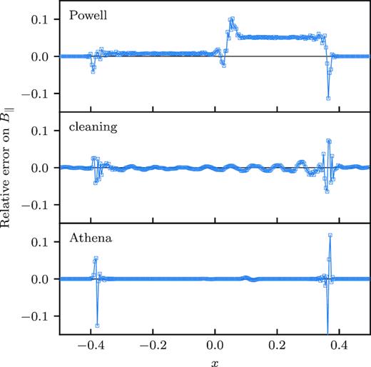
$Rotated shock tube test. The relative error on the parallel magnetic field $\boldsymbol B_\parallel$ in the rotated shock tube test of Tóth (2000) is shown for the DG-3 method with the Powell and hyperbolic cleaning schemes in the top and centre panels. The bottom panel shows the solution obtained with athena, with the third-order CTU (constrained transport) method. For the Powell method, between the left and right fast shocks (x = ∓0.4), the value of $\boldsymbol B_\parallel$ deviates with respect to the exact solution due to the non-conservative source terms. Apart from oscillations at the discontinuities, the Powell scheme results in systematic offsets of $\boldsymbol B_\parallel$ of order ≲5 per cent. The hyperbolic cleaning scheme features no such systematic offsets, but produces damped oscillations which overtake the fast shocks as the divergence gets advected away.$

Figure 29.

Rotated shock tube test. The relative error on the parallel magnetic field |$\boldsymbol B_\parallel$| in the rotated shock tube test of Tóth (2000) is shown for the DG-3 method with the Powell and hyperbolic cleaning schemes in the top and centre panels. The bottom panel shows the solution obtained with athena, with the third-order CTU (constrained transport) method. For the Powell method, between the left and right fast shocks (x = ∓0.4), the value of |$\boldsymbol B_\parallel$| deviates with respect to the exact solution due to the non-conservative source terms. Apart from oscillations at the discontinuities, the Powell scheme results in systematic offsets of |$\boldsymbol B_\parallel$| of order ≲5 per cent. The hyperbolic cleaning scheme features no such systematic offsets, but produces damped oscillations which overtake the fast shocks as the divergence gets advected away.

Open in new tab Download slide

For the Powell method, we find systematic errors in the 5 per cent range in the intershock region, consistent with the results of Tóth (2000). Our measured errors seem however lower than those reported by Mignone & Tzeferacos (2010) in their similar test, where they measured relative errors greater than 10 per cent. The Powell error may potentially be reduced by using a Riemann solver which propagates the divergence wave – for instance, the eight-wave Rusanov flux produces much smaller errors, but it is also extremely diffusive. We also noted in our experiments that the choice of face flux (see Section 4.1.3) plays a role in determining the location of the plateaus visible in Fig. 29, and it is possible that |$B^n_\mathrm{ F}$| may be chosen optimally as to minimize the absolute deviations in this particular test. Overall, this shows that DG cannot work around some of the pitfalls of non-conservative Powell schemes, for the fundamental reason that shocks are essentially first-order features.

The solution obtained with hyperbolic cleaning is also represented in Fig. 29. Unlike the Powell solution, it does not feature systematic shifts in the value of |$\boldsymbol B_\parallel$|⁠, however, large-scale oscillations due to the ongoing advection and damping of the divergence are visible. More importantly, these oscillations also occur for ||$x_\parallel$|| ≳ 0.4, outside of the region between the two shock fronts, which is an unphysical effect, and illustrates the fact that hyperbolic cleaning will propagate information faster than any physical MHD wave.

6 DISCUSSION

6.1 High-order schemes for astrophysics

Our tests have shown some promising results for higher order schemes in astrophysical simulations, and for MHD in particular. We now discuss how the combination of DG with AMR could allow very efficient computations in smooth regions of the flow with high-order convergence, while finely capturing the shocks and discontinuities with spatial refinement.

We can interpret order/resolution convergence plots such as Fig. 4 from two complementary points of view: looking at a given spatial resolution on the x-axis, we can increase the order to reduce the solution error. But at a fixed error on the y-axis, we may also increase the order and correspondingly reduce the spatial resolution. We argue that this second vision is more relevant to many types of simulations in astrophysics, as the spatial truncation errors need only be smaller or comparable to other types of errors, stemming from uncertainties in the physical models, missing physics, subgrid recipes, etc. We can therefore see order convergence as a way of getting away with fewer cells in smooth problems, to the extent that we can efficiently ‘patch’ smooth regions of the flow with coarser cells.

Cell-based AMR provides a suitable framework to do this, as it allows cell-by-cell resolution adaptivity to match the local feature size. In a number of our test problems, we found higher order to better resolve features close to the grid resolution. The vortex problem of Fig. 4 illustrates the advantage of higher orders for capturing features which are barely resolved by the grid (shaded area): at 32² resolution, the second-order scheme is not yet resolving the vortex, whereas the DG-4 method has already achieved its theoretical fourth-order convergence. The same conclusion holds in the presence of shocks, as illustrated by the Shu–Osher MHD shock tube in Fig. 9 where we see a significant improvement from DG-2 to DG-3. The loop advection problem further shows that sharp features (such as singular field derivatives appearing in the MHD current) can also be captured within one cell by moderately increasing the spatial order: going from second to third or fourth order dramatically improves the loop sharpness, while reducing the dissipation of magnetic energy.

Compared to Lagrangian methods, a major issue with AMR Eulerian grid codes is that they require sufficient grid resolution to avoid dissipation due to bulk flow velocities; i.e. they are only Galilean invariant for solutions sufficiently resolved to make advection errors negligible. Because spatial resolution translates into tighter CFL constraints on the time-step, a compromise has to be reached between advection errors and compute time in practice. The advected Orszag–Tang test of Section 5.3.4 demonstrates that not only do higher order schemes help reduce advection errors and restore Galilean invariance, but for smooth regions of the flow, it can actually be beneficial to increase the order while reducing spatial resolution. Note that these test problems present MHD shocks, and it is encouraging to see that these positive features remain, even though we find that they can be sensitive to the details of the limiter settings.

The combination of higher order methods with AMR therefore seems particularly powerful. We note that for most astrophysical situations, spatial refinement will likely be required, because of the presence of shocks which are inherently first-order features, but also whenever the fluid is self-gravitating. One may therefore ask what scheme order will turn out to be the optimal choice for a given problem. While we discussed positive effects of higher orders, in practice we expect diminishing returns. From the above discussion, it is clear the optimal global scheme order will depend on the volume filling fraction and geometry of shocks and other discontinuities, as well as the acceptable truncation error, both of which are very problem-dependent. Higher orders will only be helpful to the extent that we can efficiently patch smooth regions of the flow with coarser and coarser cells. In addition, the computational cost of DG becomes prohibitive for large orders, in part because of the expensive quadrature operations, but also because of the more restrictive CFL condition (27). We note that this CFL constraint can be relaxed within the DG framework, for example using so-called PNPM schemes (Dumbser et al. 2008), where N moments are evolved dynamically as in DG, whereas high-order spatial reconstruction is used up to order M ≥ N to recover the remaining moments; however this comes at the cost of a more extended pattern of ghost cells, as with purely reconstruction-based schemes.

Time integration for RKDG schemes is also both computationally and memory expensive at high temporal orders, as Runge–Kutta methods require multiple steps with intermediate storage. These memory and computational requirements may be reduced using other time integration schemes such as ADER (see Section 6.4.2). Note that even though we match the RK time integration order to the spatial order of the scheme (up to RK4) in most of our runs, this is only done to ensure that the time integration errors do not contaminate the convergence tests of Section 5.2. In practice, high-order RK time integration may be unnecessary, for example when the CFL criterion enforces very small time-steps due to high plasma temperatures, or in presence of shorter time-scales in other physical processes.

For these reasons, based on the test problems presented in this work, we expect third- or fourth-order schemes (DG-3 and DG-4) to achieve a good overall compromise when combined with AMR. Anninos et al. (2017) have reported similar practical limits for their astrophysical DG scheme, based on compute time and floating point machine precision considerations.

6.2 Discontinuous Galerkin for high order

Explicit DG schemes are often touted as a promising family of methods for high-performance computing, because they are both very local (in the sense that information about all derivatives can be obtained locally within a cell, instead of relying on multiple neighbouring cells as with reconstruction methods), and compute-intensive. Both properties are regarded as desirable in combination, as they shift the load away from the communication and memory subsystems towards CPU cores, which translates into greater parallel scalability. In addition, most of the compute operations in DG involve dense linear algebra and can be readily optimized to make use of the powerful floating point units of modern CPUs.

However, in practice, exploiting the full compute capabilities of modern CPUs, such as vector units and fused multiply add instructions, requires exposing operations to the compiler at the right level of loop granularity, which mandates careful organization of the code. In some places, we resort to temporary data structures to pack and unpack data elements to benefit from vectorization. We believe such optimization efforts are necessary if one intends to reap the benefits of DG, because of the large additional computational costs compared to reconstruction methods.

In addition to being an asset for achieving high compute efficiency, the local character of derivatives in DG could also have implications for the implementation of physical models. We find that we can obtain a very sharp and clean signal for the derivatives within a cell, as illustrated by the loop advection problem of Section 5.4.1: the MHD current is readily evaluated locally in each cell from the DG weights, and higher orders significantly improve the capturing of singular features in the current (Fig. 24). We believe this property of DG schemes could have important applications for the modelling of physical processes which require accurate derivatives of the fields, such as for example shock detection (Schaal 2016), or cosmic ray streaming in magnetic fields (e.g. Wiener, Oh & Guo 2013; Jiang & Oh 2018).

6.3 Central divergence control methods

In this paper, we have explored the implementation of cell-centred divergence control techniques, in the form of the eight-wave formalism with Powell terms, and hyperbolic divergence cleaning. We find that although these techniques can be applied successfully to MHD test problems with DG, they are no silver bullet against all divergence-related effects, in particular if we insist on using the well-tested and low-diffusion HLLD fluxes.

6.3.1 Hyperbolic divergence cleaning

We find that the hyperbolic cleaning method of Dedner et al. (2002) lends itself very well to a straightforward implementation with DG. The scheme is very effective at eliminating divergence in test problems where a single spatial and temporal scale can be readily identified. In addition, a major advantage is that we find the scheme to be equally stable with LDF but also Legendre bases for the magnetic field. As a result, hyperbolic cleaning has been a popular implementation of cell-based divergence control in DG-MHD codes (e.g. Zanotti et al. 2015; Dumbser & Loubère 2016; Kidder et al. 2017). The scheme has a number of drawbacks however, which impact its suitability for large dynamic range simulations.

First, the scheme requires at least one⁵ dimensional parameter to be set (the cleaning speed c_h), which should be chosen faster than the fastest MHD wave at all points and all times in the simulation. In the formulation of Dedner et al. (2002), c_h is taken to be uniform in space and constant in time, which is in practice intractable for simulations with large dynamic range because of the resulting global CFL constraint. Tricco et al. (2016) showed that using the original divergence cleaning formulation with time-varying c_h could result in locally creating divergence, which we have observed in our test simulations in presence of AMR. To overcome this issue, they developed locally varying cleaning speeds in both space and time in the context of Lagrangian smoothed particle hydrodynamics methods. Adapting this work to Eulerian grids could help alleviate the problem of choosing hyperbolic cleaning speeds for problems with large dynamic range.

Beyond the question of parameter tuning, hyperbolic cleaning can also produce non-physical effects, because it will propagate disturbances in the magnetic field at velocity c_h, i.e. faster than any physical wave of ideal MHD. We have seen this effect with the rotated shock tube set-up (Fig. 29). In our test problems, the effect is most impacting on the 3D blast wave problem, where the issue is compounded by the very low ambient plasma β of this particular set-up: hyperbolic cleaning will cause fluctuations in the magnetic energy to propagate outwards ahead of the shock into the background medium, resulting in a loss of positivity of the thermal pressure. In science applications, this has been found to produce spurious bending of field lines ahead of bow shocks by e.g. Susanto (2014). Approaches have been developed to address positivity issues with divergence cleaning, either by ensuring that the magnetic energy can only be decreased by the scheme (Tricco & Price 2012), or through an entropy-stable formulation with entropy variables (Derigs et al. 2018). We have not investigated these directions in this work, but leave them as potential future improvements.

6.3.2 Powell scheme

In comparison to hyperbolic divergence cleaning, the Powell source term approach does not have any free parameter, and is therefore intrinsically scale-free. We find that for most test problems, the Powell approach produces results close to hyperbolic cleaning, and in particular our implementation does not seem to suffer from some of the divergence-related problems observed by other authors with pure source term approaches (e.g. comparing the MHD blast slices of Fig. 21 with fig. 18 of Hopkins & Raives 2016, or the AMR rotor results of Fig. 19 with fig. 7 of Derigs et al. 2018). The method handles strong shocks and low plasma-β situations very robustly, as demonstrated in the 3D blast problem. Interestingly, like Balsara & Spicer (1999b), we find that isolated moving shocks are not the strongest source of divergence with the Powell scheme. Rather, interacting or standing shocks, and stagnation points in smooth flows, are most at risk of local corruption of the solution due to divergence, because the Powell scheme cannot advect it efficiently away. Typical test set-ups exhibiting these issues are the rotated shock tube and the Orszag–Tang vortex, the former featuring a standing shock, and the latter smooth stagnating flows, ‘pinch’ points, and interacting shocks.

An obvious drawback of the Powell method is its non-conservative character due to the source term which injects conserved quantities. It is difficult to comprehensively assess the exact impact of this source term on the quality of the solution. In terms of global conservation, we found only a small impact of the source term in the Orszag–Tang vortex problem (Fig. 13), but we stress that the impact could get more severe over long time-scales. The rotated shock tube provides an even more stringent test of local conservation properties, and we measure systematic deviations of about |$5 {{\ \rm per\ cent}}$| in the magnetic field strength along the problematic direction. We note that this error does not converge away with scheme order, since the shock is intrinsically a first-order feature. In addition, we also observe that this error is constant with resolution as noted by Tóth (2000), because it is caused by the effect of the integrated Powell term which is singular at the jump, and for which the cell size only acts as a regularization scale. However, outside of shocks where the solution is smooth (possibly with steep gradients), additional resolution produces smaller jumps at interfaces, thereby reducing the overall amount of divergence. This is consistent with the findings of other studies (e.g. Pakmor & Springel 2013; Zhu et al. 2015). In addition to resolution, we showed that increasing the scheme order can very efficiently reduce the divergence in smooth regions of the flow, as soon as the flow features are at least partially resolved (Fig. 5).

These non-conservative properties are a known weak point of Powell schemes, and our study shows that DG and higher order methods are not immune to them. Our Powell scheme seems however very robust in high-Mach, low-β environments, as illustrated by the 3D blast test. We note that non-conservative source terms seem to be a recurring ingredient of cell-centred schemes with good positivity properties. Mignone & Tzeferacos (2010) noticed that the behaviour of hyperbolic cleaning in the presence of shocks is improved by the addition of source terms (the co-called EGLM approach of Dedner et al. 2002). Interestingly, entropy stability – which is related to positivity and robust behaviour at shocks – seems to call for non-conservative source terms, which are themselves at odds with the underlying foundational formulation as conservation laws (Chandrashekar & Klingenberg 2016; Derigs et al. 2018).

The divergence control provided by the Powell scheme with our DG method is unfortunately not a turnkey solution. While we did not experience divergence runaways with LDF bases and the Powell term prescriptions discussed in Section 4.1.3 across all of our test runs, the resulting solutions can, for some limiter settings, show signs of divergence damage when compared to runs with hyperbolic cleaning. Generally speaking, if the characteristic slope limiter threshold |$\tilde{M}$| is set too high (i.e. if the limiter is too lenient), spurious extrema will contaminate all waves in the solution, a problem which is of course not specific to the magnetic field divergence. The current sheet problem of Section 5.4.2 illustrates a case where the Powell method suffers from too permissive limiter settings. We also noticed, however, that |$\tilde{M}$| may conversely be set too low, so that the limiter becomes too aggressive and restricts the propagation of the eighth divergence wave, thereby reducing the efficiency of divergence control. This can paradoxically result in divergence damage being greater with a more aggressive limiter setting. This effect seems particularly noticeable on the Orszag–Tang vortex problem. This does not happen with other variables or MHD waves, because they do not rely on one of the characteristics for stabilization against a runaway process.

Another important and likely related aspect of the Powell scheme in our DG implementation is that it seems to require LDF bases to achieve stability. Expanding the magnetic field components on a Legendre basis, and accounting for a volume contribution of the Powell term to the DG integrals is not sufficient to ensure stability, and can result in uncontrolled divergence blow-up.

These effects highlight the complex interactions between different ingredients of the Powell scheme, which we attribute to the non-linear nature of the Powell source term. We note that the slope limiter used in this work is rather primitive, and other limiters could well help resolve this issue. We review some possible limiter improvements in the dedicated discussion Section 6.4.1.

6.3.3 Locally divergence-free bases

As discussed above, we find that the LDF basis functions discussed in this paper are necessary for the stability of our Powell scheme. They are, however, in no way sufficient as soon as a non-diffusive Riemann solver such as HLLD is employed. More diffusive Riemann solvers, such as Rusanov fluxes, or entropy-stable fluxes of Chandrashekar & Klingenberg (2016), can achieve stability with LDF bases and no other divergence treatment on simple problems: these fluxes are generally more diffusive than HLLD, and in particular include a normal component flux for the magnetic field which will dampen the normal jump of |$\boldsymbol B$| at the faces. However, in the presence of strong shocks, we find that the HLLD solver provides sharper solutions, and therefore constitutes a more sensible choice for high-order codes attempting to resolve features close to the grid resolution.

LDF basis functions require significant additional complexity in the code and in the scheme itself, from basis function generation (see Appendix A) to special limiting procedures (such as the one we introduced in Section 4.2.4). Because LDF bases make use of the divergence-free condition, they require somewhat less storage than a componentwise Legendre basis for |$\boldsymbol B$|⁠.

However, LDF bases turn out to be potentially more computationally expensive than Legendre bases for high orders: the Legendre basis (13) possesses a tensor product structure (component × basis function) which allows optimized computation of conserved states |$\boldsymbol u$| and Gaussian quadrature using sum factorization (see Kronbichler et al. 2017). These optimizations cannot be readily used with LDF bases, because the coupling between components of |$\boldsymbol B$| breaks the tensor product structure. In addition, pre-computing and storing basis function values and gradients at quadrature points requires more memory for the LDF basis than the Legendre basis, because all three components of |$\boldsymbol B$| have to be stored (in addition to the Legendre basis, which is still required for hydro variables). The memory footprint of the precomputed basis function data can exceed the size of the L1 processor cache, and for orders ≥4 in 3D, the quadrature data for the LDF + Powell scheme will not even fit in a 256 kB L2 cache, resulting in a strong performance degradation. From a few practical tests, we find that sum factorization optimizations and careful memory footprint management can make a significant difference for orders ≥4, so users of very high-order schemes may want to reconsider the use of divergence-free bases on computational efficiency grounds.

Finally, the convergence tests of Section 5.2 have shed light on a subtle instability with LDF bases that reveals itself with HLLD fluxes in non-grid-aligned configurations. We speculate that this may be related to the projection effects discussed in Appendix B. While we do not see this as a source of concern for actual simulations, we note that the effective convergence order with LDF bases may in some cases be lower than expected.

6.3.4 Conclusion on divergence control

A natural way around the shortcomings of both schemes would be to rely on exactly globally divergence-free schemes. Such methods have been proposed for DG, for example based on vector potential techniques (e.g. Rossmanith 2013). High-order versions of constrained transport have also been developed, where the magnetic field is expanded on the interfaces, reconstructed within the cell using a divergence-free reconstruction, and evolved using a distinct evolution equation (see e.g. Li et al. 2011; Balsara & Käppeli 2017). These methods involve complicated ingredients: they require more complex mesh structures, multidimensional Riemann solvers to obtain the electric fields, and higher order expansions for the magnetic field inside the cells. In addition, because the dynamical degrees of freedom are split between cell- and face-centred discretizations, it is less clear how to define a proper limiting procedure for high-order modes.

Although we find that both hyperbolic cleaning and the Powell methods have shortcomings which are a source for concern for large dynamic range simulations, we note that these methods have been successfully used in practice in production in a finite-volume context. The extensive code comparison study of Kritsuk et al. (2011), focusing on decaying isothermal supersonic turbulence, showed no significant systematic effect of the divergence control method on a number of physically relevant quantities; the authors demonstrate that other aspects of codes are more important for accurate turbulence simulations. In particular, they find that high-order codes achieve increased spectral bandwidth and effective Reynolds number. In the context of the magnetorotational instability (MRI), Flock et al. (2010) see little difference between Powell and upwinded constrained transport schemes on MRI growth rates and evolution of the magnetic energy.

In any case, we plan to apply both hyperbolic divergence cleaning and the Powell scheme to MHD turbulence simulations, for which the impact of divergence control can be readily tested against published results.

6.4 Future improvements

Our current DG scheme relies on a number of simple ingredients which will likely require improvement for use in production astrophysical science applications. The main current directions will be to replace the simple DG limiter described in Section 4.2 by more sophisticated alternatives, add support for local time-stepping, and improve |${\nabla }{\cdot }{\boldsymbol B}$| control, even within the framework of cell-centred divergence control schemes. Fortunately, solutions to some of these issues have already been developed in the DG context, and we plan to implement them as future improvements.

6.4.1 Limiters

Our limiting procedure discussed in Section 4.2 relies on the choice of a dimensional parameter |$\tilde{M}$| (or equivalently M), which, although sufficient for smooth test problems where a single spatial scale dominates, is not convenient for problems involving large dynamic range, or for which the spatial variation of the solution is not well controlled. In addition, acting as a slope limiter, it can only ever retain second-order information in the cell whenever the limiter is triggered.

A number of more sophisticated limiters have been developed and successfully applied in the DG literature. In particular, it is possible to limit the DG solution while preserving all its higher order moments. Such limiters were first introduced as a natural extension of the TVD limiter, for example by Biswas, Devine & Flaherty (1994) and Krivodonova (2007). One advantage of these limiters is that they do not require a dimensional threshold parameter M.

Another interesting approach comes from the so-called WENO schemes, whose weighted stencils may be used to reconstruct high-order solutions with reduced oscillations (see e.g. Qiu & Shu 2004; Balsara et al. 2007; Zhong & Shu 2013). Divergence-free WENO reconstruction schemes have been developed for MHD (Balsara & Dumbser 2015; Zhao & Tang 2017), and could form a suitable basis for DG limiters with LDF bases.

More recently, so-called a posteriori subcell limiters have been developed by Clain, Diot & Loubère (2011), Sonntag & Munz (2014), Dumbser et al. (2014), and Dumbser & Loubère (2016). They rely on after-the-fact detection of solution defects by first taking a time-step and projecting the resulting tentative solution in each cell on to a finer subcell grid. The subcell grid is then inspected for loss of positivity or spurious oscillations. In case any subcell is marked as troubled, the solution in the parent cell is rolled back to the previous time point, its subcell values are recomputed and evolved in time using a lower order but more robust scheme, and the updated subcell grid is used to reconstruct the DG moments of the parent cell at the final time. This technique has been successfully used for DG implementations of MHD (Zanotti et al. 2015; Fambri et al. 2018). In particular, simple criteria for solution admissibility have been developed, and subcell oscillation detection can be performed without dimensional parameters (Dumbser et al. 2014). We intend to replace our current limiter with this promising technique in the near future.

6.4.2 Local time-stepping with ADER

While some astrophysical problems only span a limited range of spatial and temporal scales (e.g. simulations of idealized isotropic isothermal turbulence in absence of self-gravity), many simulation set-ups require spatial resolution with AMR, or feature strongly locally varying signal speeds. In the latter case, the CFL constraint (27) will impose a maximum Δt which can vary significantly across cells, and it becomes beneficial to update each cell at its own pace according to its maximal Δt using local time-stepping.

The RKDG method used in our scheme is not easily amenable to local time-stepping, because it treats the whole hyperbolic problem as a set of coupled ordinary differential equations through the semidiscrete scheme (26), in which the whole vector of all cell weights is integrated forward in time using a Runge–Kutta method.

In the DG context, local time-stepping may be achieved using the so-called ADER methods, introduced by Titarev & Toro (2002), Dumbser & Munz (2006), Dumbser, Käser & Toro (2007), and more recently reformulated by Dumbser et al. (2008). In its modern variant, ADER exploits a DG-like weak formulation on a high-order space–time basis to first obtain a high-order predictor state local to each cell. This state is then used within the DG framework to perform time integration as a predictor–corrector scheme. This formulation has been used by e.g. Zanotti et al. (2015) and Fambri, Dumbser & Zanotti (2017) to develop ADER-DG codes with AMR and local time-stepping. Very recently, Charrier & Weinzierl (2018) have shown that this ADER-DG predictor–corrector time integration scheme can be made efficient on HPC architectures, with a reduced memory footprint, increased compute intensity and optimized distributed memory data exchanges. The above properties make ADER an attractive time integration algorithm for large dynamic range astrophysical applications, as an improvement over our current RKDG scheme.

6.4.3 Divergence control

We have discussed divergence control in detail in Section 6.3. Short of implementing a full-fledged high-order version of constrained transport, we would like to try to adapt improvements of the hyperbolic cleaning methodology (following Mignone & Tzeferacos 2010; Tricco & Price 2012; Tricco et al. 2016) to a Eulerian DG framework, to allow fully adaptive cleaning speeds, and to reduce positivity issues with hyperbolic cleaning for very strong shocks. For the Powell approach, a promising direction would be to experiment with an eight-wave version of the HLLD flux, such as proposed by Fuchs et al. (2011).

7 CONCLUSIONS

In this paper, we have described our implementation of a DG scheme with AMR for MHD, implemented within the framework of the astrophysical code arepo. Our scheme relies on the Runge–Kutta DG framework, and can use two different types of cell-centred divergence control techniques: locally divergence-free bases for the magnetic field together with Powell terms to control the global divergence, and hyperbolic cleaning, which may be used with the same Legendre basis functions used for hydrodynamical variables. We have introduced two main new numerical ingredients: a non-linear limiting procedure for the magnetic field components, and different discretizations of the Powell source term, which we found to be a key ingredient for the stability and accuracy of the scheme. We have also discussed some subtle numerical and performance-related properties of LDF bases, which we encountered during our development of the scheme.

We have shown that the resulting method is accurate across a wide range of typical MHD test problems, and can achieve the expected theoretical order of convergence. Like previous authors, we found that higher order schemes can efficiently reduce advection errors in Eulerian grid codes, and we further showed that these results hold even with a simple limiting procedure and in presence of MHD shocks.

We showed that increasing the DG order of the scheme can benefit solutions which are barely resolved by the grid size, by reducing not only numerical diffusion but also magnetic field divergence more efficiently than can be achieved by increasing grid resolution. We argue that this makes higher order methods very attractive for resolution-limited astrophysical simulations. In addition, DG provides instant access to local derivatives within the cell without smearing across neighbour stencils, which can be important for astrophysical applications where a clean derivative signal is required for the physics, such as shock detection or models of cosmic ray streaming.

We discussed the divergence control performance of the Powell scheme and hyperbolic cleaning, and found that while both methods perform well across most test problems, neither of them in our current implementation was fully satisfactory across all flow regimes.

Finally, we covered a few of the future improvements planned for our current DG implementation, which we see as a base development platform for increasingly sophisticated high-order solvers in the arepo code, in which to integrate more and more physical models while developing the solvers into highly scalable implementations.

We are now planning to further test and improve the scheme with high-resolution simulations of MHD turbulence, which will provide insights on the effectiveness of our numerical ingredients – in particular the two divergence control techniques – and more generally contribute to shedding light on the potential of DG methods for astrophysics.

ACKNOWLEDGEMENTS

TG would like to thank Markus Zenk, Philipp Girichidis, Christoph Pfrommer, Matthew Bate, and Pascal Tremblin for very helpful discussions. The authors would also like to thank the anonymous referee for their careful reading and helpful comments which have contributed to significantly improving the manuscript. The authors gratefully acknowledge the support of the Klaus Tschira Foundation. We acknowledge financial support through subproject EXAMAG of the Priority Programme 1648 ‘SPPEXA’ of the German Science Foundation, and through the European Research Council through ERC-StG grant EXAGAL-308037. This work was also partly supported by the European Research Counciladvanced grant no. 787361-COBOM. PC acknowledges support from the Airbus Foundation Chair on Mathematics of Complex Systems at TIFR-CAM, Bangalore.

Footnotes

1

Note that using β = 1 with the TVB limiter is not a suitable choice in practice. As resolution is increased, the MΔx² threshold will protect only O(1) cells around local extrema from the minmod function, and as a result the latter will end up being invoked almost everywhere in the domain. If β = 1, then minmod(a, b, c) ≠ a almost everywhere, which will end up triggering the limiter on almost all cells of the domain, degrading the scheme to second order at best.

2

Note that since we use an even number of grid points per dimension, we here simply approximate the slices as the average of the two rows (or columns) of cells immediately adjacent to the box centre line.

3

Note that Balsara et al. (2009) mention |$1000 \sqrt{3}^{-1}$| for B₀ in the text, but their figure seems to correspond to |$100 \sqrt{3}^{-1}$| instead.

4

https://www.astro.princeton.edu/∼jstone/Athena/tests/current-sheet/current-sheet.html.

5

As discussed in Section 4.1.5, our current implementation requires three dimensional parameters, but they can be reduced to only one using the parametrization of Mignone & Tzeferacos (2010).

REFERENCES

Anninos

P.

,

Bryant

C.

,

Fragile

P. C.

,

Holgado

A. M.

,

Lau

C.

,

Nemergut

D.

,

2017

,

ApJS

,

231

,

17

10.3847/1538-4365/aa7ff5

Crossref

Search ADS

Balsara

D. S.

,

1998

,

ApJS

,

116

,

133

10.1086/313093

Crossref

Search ADS

Balsara

D. S.

,

2004

,

ApJS

,

151

,

149

10.1086/381377

Crossref

Search ADS

Balsara

D. S.

,

2009

,

J. Comput. Phys.

,

228

,

5040

10.1016/j.jcp.2009.03.038

Crossref

Search ADS

Balsara

D. S.

,

2017

,

Living Rev. Comput. Astrophys.

,

3

,

2

10.1007/s41115-017-0002-8

Crossref

Search ADS

PubMed

Balsara

D. S.

,

Dumbser

M.

,

2015

,

J. Comput. Phys.

,

299

,

687

10.1016/j.jcp.2015.07.012

Crossref

Search ADS

Balsara

D. S.

,

Käppeli

R.

,

2017

,

J. Comput. Phys.

,

336

,

104

10.1016/j.jcp.2017.01.056

Crossref

Search ADS

Balsara

D. S.

,

Shu

C.-W.

,

2000

,

J. Comput. Phys.

,

160

,

405

10.1006/jcph.2000.6443

Crossref

Search ADS

Balsara

D. S.

,

Spicer

D.

,

1999a

,

J. Comput. Phys.

,

148

,

133

10.1006/jcph.1998.6108

Crossref

Search ADS

Balsara

D. S.

,

Spicer

D. S.

,

1999b

,

J. Comput. Phys.

,

149

,

270

10.1006/jcph.1998.6153

Crossref

Search ADS

Balsara

D. S.

,

Altmann

C.

,

Munz

C.-D.

,

Dumbser

M.

,

2007

,

J. Comput. Phys.

,

226

,

586

10.1016/j.jcp.2007.04.032

Crossref

Search ADS

Balsara

D. S.

,

Rumpf

T.

,

Dumbser

M.

,

Munz

C.-D.

,

2009

,

J. Comput. Phys.

,

228

,

2480

10.1016/j.jcp.2008.12.003

Crossref

Search ADS

Bauer

A.

,

Springel

V.

,

2012

,

MNRAS

,

423

,

2558

10.1111/j.1365-2966.2012.21058.x

Crossref

Search ADS

Biswas

R.

,

Devine

K. D.

,

Flaherty

J. E.

,

1994

,

Appl. Numer. Math.

,

14

,

255

10.1016/0168-9274(94)90029-9

Crossref

Search ADS

Boscheri

W.

,

Dumbser

M.

,

2017

,

J. Comput. Phys.

,

346

,

449

10.1016/j.jcp.2017.06.022

Crossref

Search ADS

Boscheri

W.

,

Dumbser

M.

,

Balsara

D.

,

2014

,

Int. J. Numer. Methods Fluids

,

76

,

737

10.1002/fld.3947

Crossref

Search ADS

Brackbill

J. U.

,

Barnes

D. C.

,

1980

,

J. Comput. Phys.

,

35

,

426

10.1016/0021-9991(80)90079-0

Crossref

Search ADS

Brio

M.

,

Wu

C. C.

,

1988

,

J. Comput. Phys.

,

75

,

400

10.1016/0021-9991(88)90120-9

Crossref

Search ADS

Chakravarthy

V. K.

,

Arora

K.

,

Chakraborty

D.

,

2015

,

Int. J. Numer. Methods Fluids

,

77

,

707

10.1002/fld.4000

Crossref

Search ADS

Chandrashekar

P.

,

Klingenberg

C.

,

2016

,

SIAM J. Numer. Anal.

,

54

,

1313

10.1137/15M1013626

Crossref

Search ADS

Charrier

D. E.

,

Weinzierl

T.

,

2018

, preprint (arXiv:1801.08682)

cs.MS

Clain

S.

,

Diot

S.

,

Loubère

R.

,

2011

,

J. Comput. Phys.

,

230

,

4028

10.1016/j.jcp.2011.02.026

Crossref

Search ADS

Cockburn

B.

,

Shu

C.

,

1998

,

SIAM J. Numer. Anal.

,

35

,

2440

10.1137/S0036142997316712

Crossref

Search ADS

Cockburn

B.

,

Shu

C.-W.

,

1989

,

Math. Comput.

,

52

,

411

10.2307/2008474

Crossref

Cockburn

B.

,

Lin

S.-Y.

,

Shu

C.-W.

,

1989

,

J. Comput. Phys.

,

84

,

90

10.1016/0021-9991(89)90183-6

Crossref

Search ADS

Cockburn

B.

,

Li

F.

,

Shu

C.-W.

,

2004

,

J. Comput. Phys.

,

194

,

588

10.1016/j.jcp.2003.09.007

Crossref

Search ADS

Collins

D. C.

,

Xu

H.

,

Norman

M. L.

,

Li

H.

,

Li

S.

,

2010

,

ApJS

,

186

,

308

10.1088/0067-0049/186/2/308

Crossref

Search ADS

Dai

W.

,

Woodward

P. R.

,

1998

,

ApJ

,

494

,

317

10.1086/305176

Crossref

Search ADS

Dedner

A.

,

Kemm

F.

,

Kröner

D.

,

Munz

C.-D.

,

Schnitzer

T.

,

Wesenberg

M.

,

2002

,

J. Comput. Phys.

,

175

,

645

10.1006/jcph.2001.6961

Crossref

Search ADS

Derigs

D.

,

Winters

A. R.

,

Gassner

G. J.

,

Walch

S.

,

2016

,

J. Comput. Phys.

,

317

,

223

10.1016/j.jcp.2016.04.048

Crossref

Search ADS

Derigs

D.

,

Winters

A. R.

,

Gassner

G. J.

,

Walch

S.

,

Bohm

M.

,

2018

,

J. Comput. Phys.

,

364

,

420

10.1016/j.jcp.2018.03.002

Crossref

Search ADS

Dubois

Y.

,

Teyssier

R.

,

2010

,

A&A

,

523

,

A72

10.1051/0004-6361/200913014

Crossref

Search ADS

Dumbser

M.

,

Loubère

R.

,

2016

,

J. Comput. Phys.

,

319

,

163

10.1016/j.jcp.2016.05.002

Crossref

Search ADS

Dumbser

M.

,

Munz

C.-D.

,

2006

,

J. Sci. Comput.

,

27

,

215

10.1007/s10915-005-9025-0

Crossref

Search ADS

Dumbser

M.

,

Käser

M.

,

Toro

E. F.

,

2007

,

Geophys. J. Int.

,

171

,

695

10.1111/j.1365-246X.2007.03427.x

Crossref

Search ADS

Dumbser

M.

,

Balsara

D. S.

,

Toro

E. F.

,

Munz

C.-D.

,

2008

,

J. Comput. Phys.

,

227

,

8209

10.1016/j.jcp.2008.05.025

Crossref

Search ADS

Dumbser

M.

,

Zanotti

O.

,

Loubère

R.

,

Diot

S.

,

2014

,

J. Comput. Phys.

,

278

,

47

10.1016/j.jcp.2014.08.009

Crossref

Search ADS

Evans

C. R.

,

Hawley

J. F.

,

1988

,

ApJ

,

332

,

659

10.1086/166684

Crossref

Search ADS

Fambri

F.

,

Dumbser

M.

,

Zanotti

O.

,

2017

,

Comput. Phys. Commun.

,

220

,

297

10.1016/j.cpc.2017.08.001

Crossref

Search ADS

Fambri

F.

,

Dumbser

M.

,

Köppel

S.

,

Rezzolla

L.

,

Zanotti

O.

,

2018

,

MNRAS

,

477

,

4543

10.1093/mnras/sty734

Crossref

Federrath

C.

,

Roman-Duval

J.

,

Klessen

R. S.

,

Schmidt

W.

,

Mac Low

M.-M.

,

2010

,

A&A

,

512

,

A81

10.1051/0004-6361/200912437

Crossref

Search ADS

Flock

M.

,

Dzyurkevich

N.

,

Klahr

H.

,

Mignone

A.

,

2010

,

A&A

,

516

,

A26

10.1051/0004-6361/200912443

Crossref

Search ADS

Fromang

S.

,

Hennebelle

P.

,

Teyssier

R.

,

2006

,

A&A

,

457

,

371

10.1051/0004-6361:20065371

Crossref

Search ADS

Fryxell

B.

et al. .,

2000

,

ApJS

,

131

,

273

10.1086/317361

Crossref

Search ADS

Fuchs

F. G.

,

McMurry

A. D.

,

Mishra

S.

,

Risebro

N. H.

,

Waagan

K.

,

2011

,

Commun. Comput. Phys.

,

9

,

324

10.4208/cicp.171109.070510a

Crossref

Search ADS

Gaburov

E.

,

Nitadori

K.

,

2011

,

MNRAS

,

414

,

129

10.1111/j.1365-2966.2011.18313.x

Crossref

Search ADS

Gardiner

T. A.

,

Stone

J. M.

,

2005

,

J. Comput. Phys.

,

205

,

509

10.1016/j.jcp.2004.11.016

Crossref

Search ADS

Godunov

S. K.

,

1972

,

Numer. Methods Mech. Contin. Medium

,

1

,

26

Gottlieb

S.

,

2005

,

J. Sci. Comput.

,

25

,

105

10.1007/s10915-004-4635-5

Crossref

Hawley

J. F.

,

Stone

J. M.

,

1995

,

Comput. Phys. Commun.

,

89

,

127

10.1016/0010-4655(95)00190-Q

Crossref

Search ADS

Helzel

C.

,

Rossmanith

J. A.

,

Taetz

B.

,

2011

,

J. Comput. Phys.

,

230

,

3803

10.1016/j.jcp.2011.02.009

Crossref

Search ADS

Hesthaven

J. S.

,

Warburton

T.

,

2008

,

Nodal Discontinuous Galerkin Methods: Algorithms, Analysis, and Applications. No. 54 in Texts in Applied Mathematics

.

Springer

,

New York

Google Scholar

Google Preview

OpenURL Placeholder Text

WorldCat

Hopkins

P. F.

,

2016

,

MNRAS

,

462

,

576

10.1093/mnras/stw1578

Crossref

Search ADS

Hopkins

P. F.

,

Raives

M. J.

,

2016

,

MNRAS

,

455

,

51

10.1093/mnras/stv2180

Crossref

Search ADS

Janhunen

P.

,

2000

,

J. Comput. Phys.

,

160

,

649

10.1006/jcph.2000.6479

Crossref

Search ADS

Jiang

Y.-F.

,

Oh

S. P.

,

2018

,

ApJ

,

854

,

5

10.3847/1538-4357/aaa6ce

Crossref

Search ADS

Jiang

G.-S.

,

Shu

C.-W.

,

1996

,

J. Comput. Phys.

,

126

,

202

10.1006/jcph.1996.0130

Crossref

Search ADS

Jiang

G.-S.

,

Wu

C.-c.

,

1999

,

J. Comput. Phys.

,

150

,

561

10.1006/jcph.1999.6207

Crossref

Search ADS

Karami Halashi

B.

,

Luo

H.

,

2016

,

J. Comput. Phys.

,

326

,

258

10.1016/j.jcp.2016.08.055

Crossref

Search ADS

Kemm

F.

,

2013

,

Commun. Appl. Math. Comput. Sci.

,

8

,

1

10.2140/camcos.2013.8.1

Crossref

Search ADS

Kidder

L. E.

et al. .,

2017

,

J. Comput. Phys.

,

335

,

84

10.1016/j.jcp.2016.12.059

Crossref

Search ADS

Kritsuk

A. G.

et al. .,

2011

,

ApJ

,

737

,

13

10.1088/0004-637X/737/1/13

Crossref

Search ADS

Krivodonova

L.

,

2007

,

J. Comput. Phys.

,

226

,

879

10.1016/j.jcp.2007.05.011

Crossref

Search ADS

Kronbichler

M.

,

Kormann

K.

,

Pasichnyk

I.

,

Allalen

M.

,

2017

, in

High Performance Computing. Lecture Notes in Computer Science

.

Springer

,

Cham

, p.

237

10.1007/978-3-319-58667-0_13

Google Scholar

Google Preview

OpenURL Placeholder Text

WorldCat

Crossref

LeVeque

R. J.

,

2002

,

Finite Volume Methods for Hyperbolic Problems

.

Cambridge Univ. Press

,

Cambridge

Google Scholar

Google Preview

OpenURL Placeholder Text

WorldCat

Li

F.

,

Shu

C.-W.

,

2005

,

J. Sci. Comput.

,

22-23

,

413

10.1007/s10915-004-4146-4

Crossref

Search ADS

Li

F.

,

Xu

L.

,

2012

,

J. Comput. Phys.

,

231

,

2655

10.1016/j.jcp.2011.12.016

Crossref

Search ADS

Li

F.

,

Xu

L.

,

Yakovlev

S.

,

2011

,

J. Comput. Phys.

,

230

,

4828

10.1016/j.jcp.2011.03.006

Crossref

Search ADS

Liu

Y.

,

Shu

C.-W.

,

Zhang

M.

,

2018

,

J. Comput. Phys.

,

354

,

163

10.1016/j.jcp.2017.10.043

Crossref

Search ADS

Mac Low

M.-M.

,

1999

,

ApJ

,

524

,

169

10.1086/307784

Crossref

Search ADS

Marinacci

F.

,

Vogelsberger

M.

,

Kannan

R.

,

Mocz

P.

,

Pakmor

R.

,

Springel

V.

,

2018

,

MNRAS

,

476

,

2476

10.1093/mnras/sty397

Crossref

Search ADS

Meurer

A.

et al. .,

2017

,

PeerJ. Comput. Sci.

,

3

,

e103

10.7717/peerj-cs.103

Crossref

Search ADS

Mignone

A.

,

Tzeferacos

P.

,

2010

,

J. Comput. Phys.

,

229

,

2117

10.1016/j.jcp.2009.11.026

Crossref

Search ADS

Mignone

A.

,

Bodo

G.

,

Massaglia

S.

,

Matsakos

T.

,

Tesileanu

O.

,

Zanni

C.

,

Ferrari

A.

,

2007

,

ApJS

,

170

,

228

10.1086/513316

Crossref

Search ADS

Mignone

A.

,

Zanni

C.

,

Tzeferacos

P.

,

van Straalen

B.

,

Colella

P.

,

Bodo

G.

,

2012

,

ApJS

,

198

,

7

10.1088/0067-0049/198/1/7

Crossref

Search ADS

Miyoshi

T.

,

Kusano

K.

,

2005

,

J. Comput. Phys.

,

208

,

315

10.1016/j.jcp.2005.02.017

Crossref

Search ADS

Mocz

P.

,

Vogelsberger

M.

,

Sijacki

D.

,

Pakmor

R.

,

Hernquist

L.

,

2014

,

MNRAS

,

437

,

397

10.1093/mnras/stt1890

Crossref

Search ADS

Mocz

P.

,

Pakmor

R.

,

Springel

V.

,

Vogelsberger

M.

,

Marinacci

F.

,

Hernquist

L.

,

2016

,

MNRAS

,

463

,

477

10.1093/mnras/stw2004

Crossref

Search ADS

Nelson

D.

,

Vogelsberger

M.

,

Genel

S.

,

Sijacki

D.

,

Kereš

D.

,

Springel

V.

,

Hernquist

L.

,

2013

,

MNRAS

,

429

,

3353

10.1093/mnras/sts595

Crossref

Search ADS

Pakmor

R.

et al. .,

2017

,

MNRAS

,

469

,

3185

10.1093/mnras/stx1074

Crossref

Search ADS

Pakmor

R.

,

Springel

V.

,

2013

,

MNRAS

,

432

,

176

10.1093/mnras/stt428

Crossref

Search ADS

Pakmor

R.

,

Bauer

A.

,

Springel

V.

,

2011

,

MNRAS

,

418

,

1392

10.1111/j.1365-2966.2011.19591.x

Crossref

Search ADS

Pakmor

R.

,

Marinacci

F.

,

Springel

V.

,

2014

,

ApJ

,

783

,

L20

10.1088/2041-8205/783/1/L20

Crossref

Search ADS

Powell

K. G.

,

1994

,

Technical Report, Approximate Riemann Solver for Magnetohydrodynamics (That Works in More than One Dimension)

.

NASA ICASE

,

Hampton, VA

Google Scholar

Google Preview

OpenURL Placeholder Text

WorldCat

Powell

K. G.

,

Roe

P. L.

,

Linde

T. J.

,

Gombosi

T. I.

,

De Zeeuw

D. L.

,

1999

,

J. Comput. Phys.

,

154

,

284

10.1006/jcph.1999.6299

Crossref

Search ADS

Qiu

J.

,

Shu

C.-w.

,

2004

,

SIAM J. Sci. Comput.

,

26

,

907

10.1137/S1064827503425298

Crossref

Search ADS

Rieder

M.

,

Teyssier

R.

,

2016

,

MNRAS

,

457

,

1722

10.1093/mnras/stv2985

Crossref

Search ADS

Rieder

M.

,

Teyssier

R.

,

2017

,

MNRAS

,

472

,

4368

10.1093/mnras/stx2276

Crossref

Search ADS

Robertson

B. E.

,

Kravtsov

A. V.

,

Gnedin

N. Y.

,

Abel

T.

,

Rudd

D. H.

,

2010

,

MNRAS

,

401

,

2463

10.1111/j.1365-2966.2009.15823.x

Crossref

Search ADS

Robinet

J.-C.

,

Gressier

J.

,

Casalis

G.

,

Moschetta

J.-M.

,

2000

,

J. Fluid Mech.

,

417

,

237

10.1017/S0022112000001129

Crossref

Search ADS

Rossmanith

J.

,

2006

,

SIAM J. Sci. Comput.

,

28

,

1766

10.1137/050627022

Crossref

Search ADS

Rossmanith

J. A.

,

2013

, preprint (arXiv:1310.4251)

math.NA

Ryu

D.

,

Ostriker

J. P.

,

Kang

H.

,

Cen

R.

,

1993

,

ApJ

,

414

,

1

10.1086/173051

Crossref

Search ADS

Ryu

D.

,

Miniati

F.

,

Jones

T. W.

,

Frank

A.

,

1998

,

ApJ

,

509

,

244

10.1086/306481

Crossref

Search ADS

Schaal

K.

,

2016

,

PhD thesis

,

Universität Heidelberg

Google Scholar

Google Preview

OpenURL Placeholder Text

WorldCat

Schaal

K.

,

Bauer

A.

,

Chandrashekar

P.

,

Pakmor

R.

,

Klingenberg

C.

,

Springel

V.

,

2015

,

MNRAS

,

453

,

4279

10.1093/mnras/stv1859

Crossref

Search ADS

Schekochihin

A. A.

,

Cowley

S. C.

,

Taylor

S. F.

,

Maron

J. L.

,

McWilliams

J. C.

,

2004

,

ApJ

,

612

,

276

10.1086/422547

Crossref

Search ADS

Shu

C.-W.

,

1987

,

Math. Comput.

,

49

,

105

10.1090/S0025-5718-1987-0890256-5

Crossref

Search ADS

Shu

C.-W.

,

1998

, in

Quarteroni

A.

, ed.,

Advanced Numerical Approximation of Nonlinear Hyperbolic Equations, Vol. 1697

.

Springer

,

Berlin

, p.

325

10.1007/BFb0096355

Google Scholar

Google Preview

OpenURL Placeholder Text

WorldCat

Crossref

Shu

C.-W.

,

2013

,

Adv. Mech.

,

43

,

541

Shu

C.-W.

,

Osher

S.

,

1989

, in

Upwind and High-Resolution Schemes

.

Springer

,

Berlin, Heidelberg

, p.

328

10.1007/978-3-642-60543-7_14

Google Scholar

Google Preview

OpenURL Placeholder Text

WorldCat

Crossref

Sonntag

M.

,

Munz

C.-D.

,

2014

, in

Springer Proceedings in Mathematics and Statistics, Finite Volumes for Complex Applications VII-Elliptic, Parabolic and Hyperbolic Problems

.

Springer

,

Cham

, p.

945

10.1007/978-3-319-05591-6_96

Google Scholar

Google Preview

OpenURL Placeholder Text

WorldCat

Crossref

Spiegel

S. C.

,

Huynh

H. T.

,

DeBonis

J. R.

,

2015

, in

22nd AIAA Computational Fluid Dynamics Conference

.

American Institute of Aeronautics and Astronautics

,

Dallas, TX

10.2514/6.2015-2444

Google Scholar

Google Preview

OpenURL Placeholder Text

WorldCat

Crossref

Springel

V.

,

2010

,

MNRAS

,

401

,

791

10.1111/j.1365-2966.2009.15715.x

Crossref

Search ADS

Stone

J. M.

,

Norman

M. L.

,

1992

,

ApJS

,

80

,

791

10.1086/191681

Crossref

Search ADS

Stone

J. M.

,

Ostriker

E. C.

,

Gammie

C. F.

,

1998

,

ApJ

,

508

,

L99

10.1086/311718

Crossref

Search ADS

Stone

J. M.

,

Gardiner

T. A.

,

Teuben

P.

,

Hawley

J. F.

,

Simon

J. B.

,

2008

,

ApJS

,

178

,

137

10.1086/588755

Crossref

Search ADS

Susanto

A.

,

2014

,

PhD thesis

,

University of Waterloo

Google Scholar

Google Preview

OpenURL Placeholder Text

WorldCat

Teyssier

R.

,

2002

,

A&A

,

385

,

337

10.1051/0004-6361:20011817

Crossref

Search ADS

Teyssier

R.

,

Fromang

S.

,

Dormy

E.

,

2006

,

J. Comput. Phys.

,

218

,

44

10.1016/j.jcp.2006.01.042

Crossref

Search ADS

Titarev

V. A.

,

Toro

E. F.

,

2002

,

J. Sci. Comput.

,

17

,

609

10.1023/A:1015126814947

Crossref

Search ADS

Tóth

G.

,

2000

,

J. Comput. Phys.

,

161

,

605

10.1006/jcph.2000.6519

Crossref

Search ADS

Tricco

T. S.

,

Price

D. J.

,

2012

,

J. Comput. Phys.

,

231

,

7214

10.1016/j.jcp.2012.06.039

Crossref

Search ADS

Tricco

T. S.

,

Price

D. J.

,

Bate

M. R.

,

2016

,

J. Comput. Phys.

,

322

,

326

10.1016/j.jcp.2016.06.053

Crossref

Search ADS

Velasco Romero

D. A.

,

Han Veiga

M.

,

Teyssier

R.

,

Masset

F. S.

,

2018

,

MNRAS

,

478

,

1855

10.1093/mnras/sty1192

Crossref

Search ADS

Waagan

K.

,

2009

,

J. Comput. Phys.

,

228

,

8609

10.1016/j.jcp.2009.08.020

Crossref

Search ADS

Waagan

K.

,

Federrath

C.

,

Klingenberg

C.

,

2011

,

J. Comput. Phys.

,

230

,

3331

10.1016/j.jcp.2011.01.026

Crossref

Search ADS

Wang

P.

,

Abel

T.

,

2009

,

ApJ

,

696

,

96

10.1088/0004-637X/696/1/96

Crossref

Search ADS

Wang

C.

,

Zhang

X.

,

Shu

C.-W.

,

Ning

J.

,

2012

,

J. Comput. Phys.

,

231

,

653

10.1016/j.jcp.2011.10.002

Crossref

Search ADS

Warburton

T. C.

,

Karniadakis

G. E.

,

1999

,

J. Comput. Phys.

,

152

,

608

10.1006/jcph.1999.6248

Crossref

Search ADS

Wiener

J.

,

Oh

S. P.

,

Guo

F.

,

2013

,

MNRAS

,

434

,

2209

10.1093/mnras/stt1163

Crossref

Search ADS

Winters

A. R.

,

Gassner

G. J.

,

2016

,

J. Comput. Phys.

,

304

,

72

10.1016/j.jcp.2015.09.055

Crossref

Search ADS

Xu

Z.

,

Liu

Y.

,

2016

,

J. Comput. Phys.

,

327

,

203

10.1016/j.jcp.2016.09.044

Crossref

Search ADS

Yakovlev

S.

,

Xu

L.

,

Li

F.

,

2013

,

J. Comput. Sci.

,

4

,

80

10.1016/j.jocs.2012.05.002

Crossref

Search ADS

Zanotti

O.

,

Fambri

F.

,

Dumbser

M.

,

2015

,

MNRAS

,

452

,

3010

10.1093/mnras/stv1510

Crossref

Search ADS

Zhang

X.

,

Shu

C.-W.

,

2010

,

J. Comput. Phys.

,

229

,

8918

10.1016/j.jcp.2010.08.016

Crossref

Search ADS

Zhao

J.

,

Tang

H.

,

2017

,

J. Comput. Phys.

,

343

,

33

10.1016/j.jcp.2017.04.027

Crossref

Search ADS

Zhao

X.

,

Yang

Y.

,

Seyler

C. E.

,

2014

,

J. Comput. Phys.

,

278

,

400

10.1016/j.jcp.2014.08.044

Crossref

Search ADS

Zhong

X.

,

Shu

C.-W.

,

2013

,

J. Comput. Phys.

,

232

,

397

10.1016/j.jcp.2012.08.028

Crossref

Search ADS

Zhu

W.

,

Feng

L.-l.

,

Xia

Y.

,

Shu

C.-W.

,

Gu

Q.

,

Fang

L.-Z.

,

2013

,

ApJ

,

777

,

48

10.1088/0004-637X/777/1/48

Crossref

Search ADS

Zhu

C.

,

Pakmor

R.

,

van Kerkwijk

M. H.

,

Chang

P.

,

2015

,

ApJ

,

806

,

L1

10.1088/2041-8205/806/1/L1

Crossref

Search ADS

APPENDIX A: LOCALLY DIVERGENCE-FREE BASIS

A1 Divergence-free vector space

In this section, we take D to be the number of spatial dimensions, and work in spatial coordinates of the reference cell, (ξ₁, …, ξ_D) ∈ [−1, 1]^D, which are the indeterminates of our polynomials. Let |$\mathcal {P}_{ d}$| be the vector space of D-variate polynomials of degree ≤d:

\begin{eqnarray*} \mathcal {P}_{ d} = \left\lbrace \sum _{k_1+\cdots +k_D \le d} c_{k_1 \cdots k_D} \xi _1^{k_1} \cdots \xi _D^{k_D}, \quad c_{k_1 \cdots k_D} \in \mathbb {R} \right\rbrace . \end{eqnarray*}

(A1)

This vector space has dimension:

\begin{eqnarray*} n(d) {:=} \dim \mathcal {P}_{ d} &=& \sum _{k_1+\cdots +k_D \le d} 1 \\ &=& \frac{1}{2}(d+1)(d+2) \quad \text{ for }D=2 \\ &=& \frac{1}{6}(d+1)(d+2)(d+3) \quad \text{ for }D=3. \end{eqnarray*}

(A2)

Let |$\mathcal {V}_{ d}$| be the space of polynomial vector fields of degree ≤d:

\begin{eqnarray*} \mathcal {V}_{ d} = \left\lbrace {\left[\begin{array}{c}Q_1 \\ \vdots \\ Q_{ D} \end{array}\right]}, \quad (Q_1, \ldots , Q_{ D}) \in \mathcal {P}_{ d}^D \right\rbrace , \end{eqnarray*}

(A3)

and it follows that

\begin{eqnarray*} \dim \mathcal {V}_{ d} = D \dim \mathcal {P}_{ d} = Dn(d). \end{eqnarray*}

(A4)

We are interested in |$\mathcal {V}_{ d}^\text{div}$|⁠, the vector space of divergence-free polynomial vectors:

\begin{eqnarray*} \mathcal {V}_{ d}^\text{div} = \left\lbrace \boldsymbol V \in \mathcal {V}_{ d}, \sum _{\alpha =1}^D \frac{\partial V_\alpha }{\partial \xi _\alpha } = 0 \right\rbrace . \end{eqnarray*}

(A5)

We can obtain the dimension of |$\mathcal {V}_{ d}^\text{div}$| from the rank-nullity theorem. Consider the divergence as a linear application δ:

\begin{eqnarray*} \delta : \mathcal {V}_{ d} & \rightarrow \mathcal {P}_{{ d}-1} \\ \boldsymbol V & \mapsto {\nabla }{\cdot }{\boldsymbol V}. \end{eqnarray*}

(A6)

By definition of |$\mathcal {V}_{ d}^\text{div}$|⁠, |$\mathcal {V}_{ d}^\text{div} = \text{Ker}\, \delta$|⁠. Furthermore, for any |$\boldsymbol V \in \mathcal {V}_{ d}$|⁠, |$\delta (\boldsymbol V)$| is a scalar polynomial of degree d − 1, so |$\text{Im}\, \delta \subset \mathcal {P}_{{ d}-1}$|⁠. But the reverse inclusion also holds, since for any scalar polynomial |$Q \in \mathcal {P}_{{ d}-1}$|⁠, we can construct |$\boldsymbol V \in \mathcal {V}_{ d}$| such that |$\delta (\boldsymbol V) = Q$|⁠, for example:

\begin{eqnarray*} \boldsymbol V = {\left[\begin{array}{c}\int Q \, \mathrm{d}\xi _1 \\ 0 \\ \vdots \\ 0 \end{array}\right]} \in \mathcal {V}_{ d}, \end{eqnarray*}

(A7)

from which we conclude that |$\text{Im}\, \delta = \mathcal {P}_{{ d}-1}$|⁠. Then, the rank-nullity theorem applied to δ states:

\begin{eqnarray*} \dim \mathcal {V}_{ d} &=& \dim \text{Im}\, \delta + \dim \text{Ker}\, \delta \\ &=& \dim \mathcal {P}_{{ d}-1} + \dim \mathcal {V}_{ d}^\text{div}, \end{eqnarray*}

(A8)

from which we find:

\begin{eqnarray*} N_\text{div} {:=} \dim \mathcal {V}_{ d}^\text{div} = D n(d) - n(d-1). \end{eqnarray*}

(A9)

A2 Generation of basis functions

Table A1 shows the number of divergence-free basis functions for D ∈ {2, 3} and some values of the degree d. The number of basis functions grows rapidly with d, and determining them manually quickly becomes error prone, if not intractable. In addition, we not only need the functions |$\boldsymbol \phi _{ l}$| but also their D spatial derivatives and the diagonal of the mass matrix. We therefore resort to symbolic computation using the python package sympy (Meurer et al. 2017) to compute all the required symbolic expressions and generate corresponding c code.

Table A1.

Open in new tab

Number N_div of divergence-free basis functions, corresponding to the number of degrees of freedom for the magnetic field, as a function of the number of spatial dimensions D and polynomial degree d.

	N_div
d	0	1	2	3	4
D
2	2	5	9	14	20
3	3	11	26	50	85

	N_div
d	0	1	2	3	4
D
2	2	5	9	14	20
3	3	11	26	50	85

Table A1.

Open in new tab

Number N_div of divergence-free basis functions, corresponding to the number of degrees of freedom for the magnetic field, as a function of the number of spatial dimensions D and polynomial degree d.

	N_div
d	0	1	2	3	4
D
2	2	5	9	14	20
3	3	11	26	50	85

	N_div
d	0	1	2	3	4
D
2	2	5	9	14	20
3	3	11	26	50	85

We adopt a simple, brute-force approach to basis function generation, which we now illustrate in 3D for clarity. We start by choosing a sequence {Q_i} of n(d + 1) polynomials which form a basis of |$\mathcal {P}_{{ d}+1}$|⁠. At this stage, we can choose the Legendre polynomials, or simply the canonical basis of monomials. We then generate a pool of vectors of |$\mathcal {V}_{{ d}+1}$| of the form:

\begin{eqnarray*} \left\lbrace {\left[\begin{array}{c}Q \\ 0 \\ 0 \end{array}\right]}, Q \in \lbrace Q_{ i} \rbrace \right\rbrace &\cup& \left\lbrace {\left[\begin{array}{c}0 \\ Q \\ 0 \end{array}\right]}, Q \in \lbrace Q_{ i} \rbrace \right\rbrace\nonumber\\ &\cup& \left\lbrace {\left[\begin{array}{c}0 \\ 0 \\ Q \end{array}\right]}, Q \in \lbrace Q_{ i} \rbrace \right\rbrace . \end{eqnarray*}

(A10)

For each vector |$\boldsymbol V$| of this pool, |$\nabla \times \boldsymbol V$| is a vector of |$\mathcal {V}_{ d}^\text{div}$| since the curl is divergence-free, and at least one degree less than |$\boldsymbol V$|⁠. We discard the |$\boldsymbol V$| whose curl vanishes, and sort the remaining |$\nabla \times \boldsymbol V$| by increasing total degree, and optionally some other arbitrary choices such as ordering of degree on vector components.

Finally, we start from the first (lowest degree) vector polynomial in the resulting sequence, and perform a Gram–Schmidt orthogonalization of the sequence vectors with respect to the dot product:

\begin{eqnarray*} \left\langle {\boldsymbol V},{\boldsymbol W}\right\rangle = \int _{[-1,1]^3} (V_1 W_1 + V_2 W_2 + V_3 W_3) \, \mathrm{d} \boldsymbol \xi , \end{eqnarray*}

(A11)

which is exactly the dot product defined at equation (10) restricted to the components of the magnetic field. Once we have collected N_div mutually orthogonalized non-null vectors, the process is complete and we have obtained an orthogonal basis of |$\mathcal {V}_{ d}^\text{div}$|⁠, sorted by increasing total degree.

APPENDIX B: PROJECTION EFFECTS WITH LDF BASES

In this section, we illustrate that care should be taken when L²-projecting non-divergence-free functions on to LDF basis vectors. Such a situation could arise for example with our Powell scheme, when projecting limited solutions back on to DG weights, as discussed in Section 4.2.4.

The main issue with these projections is that lower degree contributions can contaminate higher degree terms. Table B1 illustrates this effect with a simple first-degree 2D vector field |$\boldsymbol u = (ax, by)$| by showing the projections |$\int _K \boldsymbol u \cdot \boldsymbol \phi _{ l}$| for each 2D LDF basis function |$\boldsymbol \phi _{ l}$|⁠. Note that |$\nabla \cdot \boldsymbol u = a+b$|⁠, and even though |$\boldsymbol u$| has only degree 1, the projection can impact arbitrarily high degrees of the LDF basis whenever a + b ≠ 0. This effect is due to the LDF basis not spanning the whole space of polynomial vector fields, and can be seen as a special form of polynomial aliasing with LDF bases.

Table B1.

Open in new tab

Contamination of higher order coefficients resulting from the L² projection of |$\boldsymbol u = (ax, by)$| on to an LDF basis.

Degree	LDF basis index l	Projection
0	0	0
	1	0
1	2	0
	3	0
	4	\|$\frac{4}{3} \left(a - b\right)$\|
2	5	0
	6	0
	7	0
	8	0
3	9	0
	10	0
	11	\|$\frac{152}{249} \left(a + b\right)$\|
	12	\|$- \frac{2}{3} \left(a + b\right)$\|
	13	0
4	14	0
	15	0
	16	0
	17	0
	18	0
	19	0
5	20	0
	21	0
	22	\|$\frac{1268}{28629} \left(a + b\right)$\|
	23	\|$- \frac{2}{45} \left(a + b\right)$\|
	24	\|$- \frac{220}{121263} \left(a + b\right)$\|
	25	0
	26	0

Degree	LDF basis index l	Projection
0	0	0
	1	0
1	2	0
	3	0
	4	\|$\frac{4}{3} \left(a - b\right)$\|
2	5	0
	6	0
	7	0
	8	0
3	9	0
	10	0
	11	\|$\frac{152}{249} \left(a + b\right)$\|
	12	\|$- \frac{2}{3} \left(a + b\right)$\|
	13	0
4	14	0
	15	0
	16	0
	17	0
	18	0
	19	0
5	20	0
	21	0
	22	\|$\frac{1268}{28629} \left(a + b\right)$\|
	23	\|$- \frac{2}{45} \left(a + b\right)$\|
	24	\|$- \frac{220}{121263} \left(a + b\right)$\|
	25	0
	26	0

Table B1.

Open in new tab

Contamination of higher order coefficients resulting from the L² projection of |$\boldsymbol u = (ax, by)$| on to an LDF basis.

Degree	LDF basis index l	Projection
0	0	0
	1	0
1	2	0
	3	0
	4	\|$\frac{4}{3} \left(a - b\right)$\|
2	5	0
	6	0
	7	0
	8	0
3	9	0
	10	0
	11	\|$\frac{152}{249} \left(a + b\right)$\|
	12	\|$- \frac{2}{3} \left(a + b\right)$\|
	13	0
4	14	0
	15	0
	16	0
	17	0
	18	0
	19	0
5	20	0
	21	0
	22	\|$\frac{1268}{28629} \left(a + b\right)$\|
	23	\|$- \frac{2}{45} \left(a + b\right)$\|
	24	\|$- \frac{220}{121263} \left(a + b\right)$\|
	25	0
	26	0

Degree	LDF basis index l	Projection
0	0	0
	1	0
1	2	0
	3	0
	4	\|$\frac{4}{3} \left(a - b\right)$\|
2	5	0
	6	0
	7	0
	8	0
3	9	0
	10	0
	11	\|$\frac{152}{249} \left(a + b\right)$\|
	12	\|$- \frac{2}{3} \left(a + b\right)$\|
	13	0
4	14	0
	15	0
	16	0
	17	0
	18	0
	19	0
5	20	0
	21	0
	22	\|$\frac{1268}{28629} \left(a + b\right)$\|
	23	\|$- \frac{2}{45} \left(a + b\right)$\|
	24	\|$- \frac{220}{121263} \left(a + b\right)$\|
	25	0
	26	0

APPENDIX C: DIVERGENCE

C1 A prescription for the amount of divergence

Different prescriptions to estimate the global divergence of the magnetic field have been proposed in the context of MHD or DG schemes (see e.g. Cockburn et al. 2004; Winters & Gassner 2016). In this work, we adopt a definition suitable to DG methods which is similar to that given in section 2.1 of Cockburn et al. (2004). We define the divergence of the magnetic field in a cell K of volume V_K as:

\begin{eqnarray*} \left| {\nabla }{\cdot }{\boldsymbol B}\right|_K {:=} \frac{1}{V_\mathrm{ K}} \int _{K} \left| {\nabla }{\cdot }{\boldsymbol B}\right| \, \mathrm{d} \boldsymbol x+ \frac{1}{V_\mathrm{ K}} \int _{\partial K} \left| B^n_\mathrm{ F} - B^n\right| \, \mathrm{d} S, \end{eqnarray*}

(C1)

where |$B^n= {B}{\cdot }{\boldsymbol n}$| with |$\boldsymbol n$| the face normal vector, and |$B^n_\mathrm{ F}$| is the normal component of the magnetic field at the face (see Section 4.1.3). The first integral is the L¹ norm of the divergence inside the cell volume, while the second is the L¹ norm of the jump in the normal magnetic field component over all faces of the cell. The face value |$B^n_\mathrm{ F}$| is used here as a way to distribute the total jump |$B^n_\mathrm{ R} - B^n_\mathrm{ L}$| between neighbouring cells L and R in a way that is consistent with the face value seen by the Riemann solver (see Fig. 3). The face and volume integrals are computed with the same Gauss–Legendre quadrature used in the DG scheme (see Schaal et al. 2015).

We define the global divergence norm of the solution over all cells in the simulation volume as:

\begin{eqnarray*} \left\Vert {\nabla }{\cdot }{\boldsymbol B}\right\Vert _1 {:=} \frac{1}{V} \sum _K V_\mathrm{ K} \left| {\nabla }{\cdot }{\boldsymbol B}\right|_\mathrm{ K}. \end{eqnarray*}

(C2)

This definition corresponds to the norm of the divergence given in section 2.1 of Cockburn et al. (2004) whenever |$B^n_\mathrm{ F} \in \left[ B^n_\mathrm{ L}, B^n_\mathrm{ R} \right]$|⁠, which is the case for both definitions of |$B^n_\mathrm{ F}$| proposed in Section 4.1.3. As noted by Cockburn et al. (2004), |$\left\Vert {\nabla }{\cdot }{\boldsymbol B}\right\Vert _1 = 0$| implies that the field is exactly globally divergence free everywhere, and as such it is a stringent measure of the amount of divergence present in the solution.

C2 Normalized divergence

Following other authors (e.g. Pakmor et al. 2011; Tricco & Price 2012; Hopkins 2016, among others), we define the normalized divergence in a cell K of size Δx as

\begin{eqnarray*} \frac{\left| {\nabla }{\cdot }{\boldsymbol B}\right|_\mathrm{ K}}{\left| \boldsymbol B\right|_\mathrm{ K}} \Delta x, \end{eqnarray*}

(C3)

where |$\left| \boldsymbol B\right|_\mathrm{ K}$| is the norm of the average magnetic field in the cell. This quantity is dimensionless, and measures the relative error on the magnetic field that can be attributed to the violation of the divergence constraint in the cell. In that sense, it measures the relative severity of the magnetic field divergence.

C3 Signed divergence

Note that by definition, |$\left| {\nabla }{\cdot }{\boldsymbol B}\right|_K$| of equation (C1) is always positive. In some instances, it is useful to give a signed definition of the divergence, for example to assess the sign of the contribution of the Powell term (29) to various conserved quantities. In such cases, the local divergence can be estimated as the cell average:

\begin{eqnarray*} \left({\nabla }{\cdot }{\boldsymbol B}\right)_K {:=} \frac{1}{V} \int _{\partial K} B^n_\mathrm{ F} \, \mathrm{d} S, \end{eqnarray*}

(C4)

where the integral runs over all faces. Here, the normal component |$B^n_\mathrm{ F}$| at the face may be chosen as in Section 4.1.3 with the HLLD solver (or returned by the Riemann solver, if using an eight-wave solver which provides an interface state). This definition arises from averaging |${\nabla }{\cdot }{\boldsymbol B}$| over the cell volume, applying the divergence theorem, and setting |$\boldsymbol B{:=} \boldsymbol B_\mathrm{ F}$| at the face. It adopts the finite-volume formulation of DG, while being sensitive to the choice of normal component of |$\boldsymbol B$| which is seen by the Riemann solver. However, it is less stringent than the definition (C1) because cancellations can occur in the integral.

This article is published and distributed under the terms of the Oxford University Press, Standard Journals Publication Model (https://dbpia.nl.go.kr/journals/pages/open_access/funder_policies/chorus/standard_publication_model)

Download all slides

Month:	Total Views:
January 2019	2
February 2019	16
March 2019	9
April 2019	33
May 2019	21
June 2019	13
July 2019	17
August 2019	11
September 2019	18
October 2019	21
November 2019	14
December 2019	4
January 2020	12
February 2020	12
March 2020	3
April 2020	4
June 2020	13
August 2020	8
September 2020	2
October 2020	5
November 2020	7
December 2020	1
January 2021	8
February 2021	6
March 2021	4
April 2021	9
May 2021	3
June 2021	4
July 2021	14
August 2021	7
September 2021	4
October 2021	1
November 2021	3
December 2021	6
January 2022	1
March 2022	3
April 2022	2
May 2022	4
June 2022	19
July 2022	11
August 2022	25
September 2022	80
October 2022	76
November 2022	44
December 2022	32
January 2023	28
February 2023	11
March 2023	21
April 2023	39
May 2023	12
June 2023	30
July 2023	13
August 2023	13
September 2023	12
October 2023	6
November 2023	18
December 2023	18
January 2024	21
February 2024	4
March 2024	17
April 2024	12
May 2024	22
June 2024	21
July 2024	48
August 2024	18
September 2024	23
October 2024	19
November 2024	14
December 2024	7
January 2025	6
February 2025	9
March 2025	19
April 2025	15
May 2025	12

Article Contents

High-order magnetohydrodynamics for astrophysics with an adaptive mesh refinement discontinuous Galerkin scheme Free

Abstract

1 INTRODUCTION

2 GOVERNING EQUATIONS

3 DISCONTINUOUS GALERKIN SCHEME

3.1 Representation of the conserved state

3.2 Legendre basis for hydrodynamics

3.3 Divergence-free basis for the magnetic field

3.4 The special case of 2D MHD

3.5 Semidiscrete DG scheme

3.6 Time integration

4 NUMERICAL INGREDIENTS

4.1 Divergence control

4.1.1 Powell source terms

4.1.2 Choice of numerical flux function

4.1.3 LDF bases and discretization of the Powell term

4.1.4 Time-step control for Powell term

4.1.5 Hyperbolic divergence cleaning

4.2 Slope limiting

4.2.1 TVB slope limiter

4.2.2 Characteristic limiting

4.2.3 Choice of limiter threshold

4.2.4 Slope limiting with LDF bases

4.3 Enforcing density and pressure positivity

4.4 Adaptive mesh refinement

5 RESULTS

5.1 General test problem set-up

5.2 Convergence order tests

5.2.1 Computing errors against analytical solution

5.2.2 Isodensity MHD vortex in 2D

5.2.3 Circularly polarized Alfvén wave problem in 2D

5.2.4 Circularly polarized Alfvén wave problem in 3D

5.3 Shock problems

5.3.1 Brio–Wu shock tube

5.3.2 1D MHD Shu–Osher test problem

5.3.3 Orszag–Tang vortex problem

5.3.4 Advected Orszag–Tang vortex

5.3.5 MHD rotor problem

5.3.6 MHD blast wave in 2D

5.3.7 MHD blast wave in 3D

5.4 Divergence control problems

5.4.1 Loop advection

5.4.2 Current sheet problem

5.4.3 Rotated shock tube

6 DISCUSSION

6.1 High-order schemes for astrophysics

6.2 Discontinuous Galerkin for high order

6.3 Central divergence control methods

6.3.1 Hyperbolic divergence cleaning

6.3.2 Powell scheme

6.3.3 Locally divergence-free bases

6.3.4 Conclusion on divergence control

6.4 Future improvements

6.4.1 Limiters

6.4.2 Local time-stepping with ADER

6.4.3 Divergence control

7 CONCLUSIONS

ACKNOWLEDGEMENTS

Footnotes

REFERENCES

APPENDIX A: LOCALLY DIVERGENCE-FREE BASIS

A1 Divergence-free vector space

A2 Generation of basis functions

APPENDIX B: PROJECTION EFFECTS WITH LDF BASES

APPENDIX C: DIVERGENCE

C1 A prescription for the amount of divergence

C2 Normalized divergence

C3 Signed divergence

Citations

Views

Altmetric

Email alerts

Astrophysics Data System

Citing articles via

Latest

Most Read

Most Cited

This Feature Is Available To Subscribers Only

High-order magnetohydrodynamics for astrophysics with an adaptive mesh refinement discontinuous Galerkin scheme