


ABSTRACT
We probe models of disc truncation in the hard spectral state of an outburst of the well-known X-ray transient GX 339–4. We test a large number of different models of disc reflection and its relativistic broadening, using two independent sets of codes, and apply it to a Rossi X-ray Timing Explorer spectrum in the rising part of the hard state of the 2010/11 outburst. We find our results to be significantly model dependent. While all of the models tested show best fits consistent with truncation, some models allow the disc to extend close to the innermost stable circular orbit (ISCO) and some require substantial disc truncation. The different models yield a wide range in best-fitting values for the disc inclination. Our statistically best model has a physical thermal Comptonization primary continuum, requires the disc to be truncated at a radius larger than or equal to about two ISCO radii for the maximum dimensionless spin of 0.998, and predicts a disc inclination in agreement with that of the binary. Our preferred models have moderate Fe abundance, ≳2 times solar. We have also tested the effect of increasing the density of the reflecting medium. We find it leads to an increase in the truncation radius, but also to an increase in the Fe abundance, opposite to a previous finding.
1 INTRODUCTION
The standard model (Novikov & Thorne 1973; Shakura & Sunyaev 1973) of accretion on to black holes (BHs) predicts formation of a viscously dissipating optically thick disc extending down to the radius of the innermost stable circular orbit (ISCO), RISCO. This model explains well soft states of accreting systems, e.g. the soft spectral state of BH X-ray binaries. However, it cannot explain states in which BH binaries and active galactic nuclei emit predominantly hard X-ray radiation (see e.g. a review by Done et al. 2007). That radiation has to be instead emitted by some hot plasma. The location of this plasma remains poorly understood.
Among accreting BH sources, low-mass BH X-ray binaries represent an important class. They are transient in most of the known cases (Coriat, Fender & Dubus 2012), and spend most of the time in a quiescent state. In that state, the optically thick disc is predicted by the disc instability model to have a large inner truncation radius, Rin ∼ 104Rg (Lasota, Narayan & Yi 1996; Dubus, Hameury & Lasota 2001), where Rg ≡ GM/c2 and M ∼ 10M|$\odot$| is the BH mass. The quiescence truncation radius has been measured in the case of the low-mass BH X-ray binary V404 Cyg to be |$R_{\rm in}\gtrsim 3.4\times 10^4 R_{\rm g}$| (Bernardini et al. 2016; see Narayan, Barret & McClintock 1997 for an earlier estimate). During quiescence, matter transferred from the companion accumulates in the disc and its inner radius continuously decreases (see e.g. fig. 13 of Dubus et al. 2001). Confirming the prediction of the decrease in Rin, an upper limit of |$R_{\rm in}\lesssim 1.2\times 10^4 R_{\rm g}$| in V404 Cyg was obtained 13 h before the onset of the 2015 X-ray outburst (Bernardini et al. 2016).
For the parameters of Dubus et al. (2001), the hydrogen-ionization instability triggering the outburst starts at a radius of ∼1010 cm (∼103Rg), a radius slightly larger than Rin at that point of time, ≈6 × 109 cm. These radii are much lower than the typical outer disc radius of ∼1011 cm, and this type of outburst is called ‘inside-out’. The truncation radius at the onset of an outburst can be estimated using observed time delays between the onsets of optical and X-ray flux rises as compared to the difference of the viscous time-scales, tvis = R2/ν (where ν is the kinematic viscosity), at the inner disc radius at the optical flux rise, Rin(V), and the X-ray one, Rin(X), with the latter assumed by Dubus et al. (2001) to be 5 × 108 cm (∼300Rg). In V404 Cyg, a ∼7-d lag has been observed by Bernardini et al. (2016), from which they derived Rin(V) ≈ 0.9–2.2 × 109 cm (∼103Rg), somewhat lower than the value of Dubus et al. (2001) and much lower than the observational upper limit obtained 13 h before the outburst (see above). An almost identical optical-to-X-ray delay, ≈7 ± 1 d, was found in a new BH transient, ASASSN-18ey, by Tucker et al. (2018), who found Rin(V) ≈ 0.8–2.5 × 109 cm.
Since the viscous time-scale decreases with decreasing radius (as |$\propto R^{1/2} T_{\rm c}^{-1}$|, where Tc is the mid-plane disc temperature, increasing with decreasing R), the assumption of the onset of X-ray outburst at Rin ≈ 5 × 108 cm has only a minor effect on the derived value of Rin(V). On the other hand, if the viscous build-up of the disc continued after the onset of the X-rays, the disc should have reached RISCO (∼106–107 cm) within a couple more days, i.e. at the beginning of the hard spectral state. We note, however, that our understanding of the mechanisms of truncation, both in quiescence and in outburst, remains very limited. The quiescence truncation radius in Dubus et al. (2001) is determined by their equation (14), from Menou et al. (2000), which, as they note, is both phenomenological and uncertain. The uncertainty is caused by our poor understanding of disc evaporation mechanisms. In the hard state, a number of different mechanisms to keep the disc truncated and change Rin with changing luminosity and source history (including a hysteretic behaviour of state transitions) have been proposed, e.g. Meyer-Hofmeister, Liu & Meyer (2005), Petrucci et al. (2008), Begelman & Armitage (2014), Kylafis & Belloni (2015), and Cao (2016). We conclude that the correct theoretical dependence of Rin on the time and luminosity after the onset of an outburst in the hard and intermediate states remains unknown.
Indeed, there is abundant evidence for the disc not reaching the ISCO at the beginning of the hard state. For example, McClintock et al. (2001) and Esin et al. (2001) found strong evidence for |$R_{\rm in}\gtrsim 50 R_{\rm g}$| 3 weeks after the beginning of the 2000 outburst of the BH binary XTE J1118+480, at a luminosity of ∼10−3 of the Eddington luminosity, LE. On the other hand, Rin certainly equals RISCO (or it is very close to it) during the soft spectral states (Ebisawa, Mitsuda & Hanawa 1991; Ebisawa et al. 1993; Gierliński & Done 2004; Steiner et al. 2011). Thus, we know that Rin has to decrease from some hundreds or ∼103Rg at the onset of the disc instability to RISCO at the onset of the soft state.
In the case of GX 339–4, a well-studied transient low-mass BH X-ray binary, a number of authors found the presence of an optically thick disc already extending very close to the ISCO in the hard spectral state at luminosities |$\gtrsim 0.01 L_{\rm E}$| (Miller et al. 2006, 2008; Reis et al. 2008; Tomsick et al. 2008; Reis, Fabian & Miller 2010; Petrucci et al. 2014; Fürst et al. 2015; García et al. 2015, hereafter G15; Wang-Ji et al. 2018b). The method used was X-ray reflection spectroscopy, in which theoretical reflection spectra are fitted to data. On the other hand, other authors found highly truncated discs in the same state using the same method, and, in some cases, using the same observations (Done & Díaz Trigo 2010; Kolehmainen, Done & Díaz Trigo 2014; Plant et al. 2015; Basak & Zdziarski 2016). A truncated disc can also explain the relatively long reverberation lags measured in the soft X-ray response of the inner disc to variability of hard X-rays (De Marco et al. 2015, 2017; Mahmoud, Done & De Marco 2018).
Some of the findings of the disc extending close to the ISCO in the luminous hard state of GX 339–4 were attributed to the effect of instrumental pile-up, present in some of the XMM–Newton fitted spectra (as discussed by Done & Díaz Trigo 2010; Kolehmainen et al. 2014; Basak & Zdziarski 2016). This effect, present in CCD detectors, is absent in the data from NuSTAR, analysed by Fürst et al. (2015) and Wang-Ji et al. (2018b). However, while Fürst et al. (2015) advocated a low truncation radius, a fraction of their best-fitting models had large truncation radii, and thus their results cannot be considered as conclusive. Then, while Wang-Ji et al. (2018b) found Rin ∼ RISCO in their models, their observations were taken in a low-luminosity state of GX 339–4, which limited the statistical significance of those results. The pile-up effect was also absent in the analysis of G15, who used data from the Proportional Counter Array (PCA) on board the Rossi X-ray Timing Explorer (RXTE). G15 used the correction to the spectral response of the PCA of García et al. (2014b) and combined hard-state PCA observations with similar X-ray fluxes, which resulted in well-calibrated spectra with very large number of counts. Then, in spite of the limited spectral resolution of the PCA (typical for proportional counters), detailed reflection spectra could be fitted. The reflection model used by G15 was then extended by Steiner et al. (2017, hereafter S17), who included the effect of scattering of the reflection photons in the hot plasma emitting the X-rays irradiating the disc. The works of G15 and S17 appear to represent some of the best documented cases for low truncation radii in the hard state of GX 339–4. However, motivated by the wealth of existing controversial results, we have embarked on an independent analysis of the PCA spectra in the hard state of GX 339–4.
GX 339–4 was discovered in 1972 (Markert et al. 1973). It has since then been the most often outbursting transient BH binary. The distance to the source, D, is relatively uncertain. Zdziarski et al. (2004) obtained |$7\, {\rm kpc}\lesssim D\lesssim 9\, {\rm kpc}$|. Heida et al. (2017) found |$D\gtrsim 5$| kpc and their preferred value was D ≈ 9 kpc. Its mass function is 1.91 ± 0.08M|$\odot$| and the mass ratio is 0.18 ± 0.05, which, with a constraint on the donor mass, give |$M \lesssim 9.5{\rm M}_{\odot }$| (Heida et al. 2017). On the other hand, Parker et al. (2016) found D ≈ 8–10 kpc and M ≈ (8–12)M|$\odot$| (including both the statistical and systematic errors) based on their X-ray spectral fits. In our estimates of the luminosity and the Eddington ratio, we assume D = 8 kpc and M = 8M|$\odot$| (as well as we assume the hydrogen fraction of 0.7 in the value of the Eddington luminosity). The binary inclination, ib, of GX 339–4 has been constrained by Heida et al. (2017) to be 37° ≤ ib ≤ 78°. We note that an inner part of the disc can be aligned with the BH rotation axis, which, in turn, can be misaligned with the binary axis. Thus, the inclination derived from X-ray fits, i, does not have to necessarily equal ib if the disc extends close to the ISCO.
2 THE DATA REDUCTION
RXTE was an X-ray observatory launched in 1996 and operational until 2012. The PCA (Jahoda et al. 2006) was one of the two pointed detectors on board RXTE. The PCA operated in the nominal energy range of 2–60 keV, and it conducted about 1400 pointed observations of GX 339–4.
We have analysed the PCA observations of GX 339–4 and extracted PCA spectra.1 We used only the Proportional Counter Unit (PCU) 2, since it was consistently operational during RXTE’s entire lifetime, as well as the best-calibrated unit. We used all of the layers of the detector. We have applied the standard dead-time correction, using the commands pcadeadcalc2 and pcadeadspect2. For each observation, we used the PCA background model for bright sources. Using the X-Ray Spectral Fitting Package (xspec) v. 12.10.0c (Arnaud 1996), we have fitted absorbed power-law models to all the spectra, and defined the spectral hardness as the ratio of the energy fluxes (from the model) between the 8.6–18 and 5–8.6 keV photon energy ranges. We show the PCA count rate as a function of that hardness in Fig. 1, where we also identify the six major outbursts of GX 339–4 observed by RXTE.
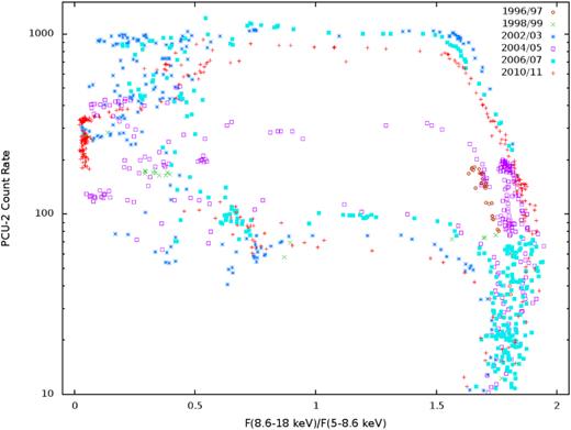
The diagram of the 3–45 keV count rate versus hardness for 1107 PCA observations of GX 339–4 during its six major outbursts, identified by different symbols and colours. The hardness is defined as the energy flux ratio of the 8.6–18 to 5–8.6 keV bands.
Then, in order to increase the statistical precision of spectral fits, we have combined spectra with similar flux and hardness. We have chosen the 2010/11 outburst, since it has the coverage of the rising part of the hard state with the highest dynamic range among all of the observed outbursts. The analysed observations are shown in Fig. 2. We started from the bottom, and included observations with increasing fluxes until a minimum of 107 counts was accumulated. In this way, we have obtained 10 sets of spectra in the hard state. We then added together observations within a set in two ways. In one, we followed the method proposed by G15. Every observation in an averaged set was fitted by an absorbed power law. The best-fitting parameters within each set were averaged and used as input parameters in fakeit command of xspec, in order to simulate an average spectrum for the continuum. The residuals were summed together, and the result added to the average absorbed power-law spectrum. For the response file, we used one of the original responses for each combined set, and we have tested that a given choice has no effect on the results. We ended up with 10 spectra at different luminosities in the hard state, which we denote using the letter G. In the second method, we obtained an summed spectrum for each set using the standard routine addspec included in the ftools package, which routine also generates the appropriate response file. The resulting spectra are denoted with the letter A. In both cases, we applied the correction to the PCA effective area of García et al. (2014b), pcacorr, and, following the recommendation of that work, added a 0.1 per cent systematic error. As shown in Section 3.3, the two procedures yield similar spectra and fitting results.

The 3–45 keV count rate versus hardness for the PCA observations of GX 339–4 during the rise of the 2010/11 outburst (which is a subset of the data shown in Fig. 1). The black circles mark the observations forming the average spectrum fitted in this work.
We have performed extensive spectral fitting with more than 10 different models for most of the spectral groups and for each of the averaging methods. We have generally found a strong model dependence of the results, and our full set of results has therefore become very complex. We have therefore decided to focus this work on showing and discussing results obtained from the analysis of only one spectrum, and defer the analysis of all the others as well as of the evolution of spectral parameters during the outburst to a follow-up paper. The chosen spectrum includes four among the brightest observations of the rising part of the outburst (see the black points in Fig. 2). The next brighter average spectrum is already located on an approximately horizontal part of the hardness-count rate diagram (together with ∼10 later observations of that outburst, see Fig. 1) and thus is likely to have different spectral properties than those characterizing the rising part. We have also checked that all of the four individual observations in the chosen average spectrum, taken on 2010 April 2, 3, 4, and 5 (Obsid 95409-01-13-03, 95409-01-13-00, 95409-01-13-04, 95409-01-13-02), have similar residuals with respect to the power-law fits. This is, e.g. not the case for the previous, fainter, spectrum, where one long observation shows much stronger residuals with respect to the fitted power-law than the remaining observations (possibly a consequence of calibration issues). Our selected spectrum has 1.01 × 10⁷ counts. Its average count rate is 705.6 s−1. It is similar in flux and hardness to spectrum B of G15 (note that the count rates given in G15 have been adjusted for the detector gain change over the lifetime of RXTE and thus cannot be directly compared with our count rate). Our spectrum has also relatively similar flux and hardness to XMM–Newton/EPIC-pn spectrum 7, taken during the same outburst on 2010 March 28 (Basak & Zdziarski 2016).
3 SPECTRAL ANALYSIS
3.1 Methodology
After preliminary spectral fitting with xspec, we used the command steppar to scan the parameter space and find the model with the overall lowest χ2. After that, we determine the 90 per cent confidence range for a single parameter, Δχ2 = +2.71, corresponding to the value farthest away from the best fit, also using steppar. Note that occasionally this procedure gives a limit within a local minimum separated from the best fit by a parameter range with Δχ2 > 2.71.
We then check for degeneracy between parameters of our models and further explore their parameter spaces using a Markov Chain Monte Carlo (MCMC) algorithm. We use the xspec_emcee implementation (by Jeremy Sanders based on Foreman-Mackey et al. 2013 and Goodman & Weare 2010). Also, we have used the standard xspec tools, for which we have tested both types of algorithms implemented, Metropolis-Hastings and Goodman-Weare, and two assumed error distributions, Gaussian and Cauchy. We have applied the MCMC method to all models in this paper, but present results graphically only for model 6, which is as presented in Section 3.6. For that, we used xspec_emcee with 50 so-called walkers with 240 000 iterations each, discarding the first 5000. The autocorrelation length calculated for each free fit parameter is approximately 80 times smaller than chain length. We note that with the MCMC we have not found any better fits than those found using steppar. We also note that the confidence ranges determined with the MCMC method in xspec usually correspond to the global minima only, and do not include possible local minima away from the global one (which we find using steppar).
The spectral fitting results for our models applied to data set G. Model 0 follows the original assumptions of G15, which appear unphysical, and model 6 is our best model, with a physical primary continuum from thermal Comptonization. All models have the ISM absorption term tbabs. Model 0: [relxill(free ZFe)+xillver(ZFe=1)]gabs; Models 1 and 2: relxill+xillver; Model 3: relxillD+xillverD; Models 4 and 5: reflkerrExp+hreflectExp; Model 6: reflkerr+hreflect. Models 0, 1, 3, 4, and 6 have high and low ionization values for the close and distant reflectors, respectively, while models 2 and 5 have the ionization structure reversed. The effect of scattering of the reflection component is taken into account in separate models with simplcut (see Section 3), for which we give here the values of the scattering fraction, fsc, in the last row of the table.
| Parameter/model | 0 | 1 | 2 | 3 | 4 | 5 | 6 |
|---|---|---|---|---|---|---|---|
| |$N_{\rm H}/10^{21}\, {\rm cm}^{-2}$| | |$5.2^{+1.8}_{-1.2}$| | |$4.7^{+1.5}_{-0.3}$| | |$6.5^{+1.3}_{-1.7}$| | |$6.1^{+0.7}_{-0.6}$| | |$4.4^{+1.9}_{-0.4}$| | |$6.4^{+0.8}_{-1.1}$| | |$4.3^{+0.5}_{-0.3}$| |
| Γ | |$1.70^{+0.07}_{-0.04}$| | |$1.66^{+0.03}_{-0.04}$| | |$1.72^{+0.02}_{-0.03}$| | |$1.70^{+0.01}_{-0.05}$| | |$1.66^{+0.06}_{-0.02}$| | |$1.72^{+0.03}_{-0.01}$| | – |
| y | – | – | – | – | – | – | |$1.19^{+0.05}_{-0.08}$| |
| Ecut/keV | |$200^{+130}_{-50}$| | |$250^{+50}_{-20}$| | |$300^{+80}_{-50}$| | 300f | |$240^{+50}_{-50}$| | |$280^{+50}_{-20}$| | – |
| |$kT_{\rm e}/1\,$|keV | – | – | – | – | – | – | |$20^{+3}_{-2}$| |
| Rin/RISCO | |$11_{-10}^{+10}$| | |$19^{+33}_{-6}$| | |$53^{+\infty }_{-26}$| | |$55^{+\infty }_{-34}$| | |$15^{+31}_{-12}$| | |$58^{+\infty }_{-28}$| | |$47^{+\infty }_{-45}$| |
| ZFe | |$8.1^{+1.9}_{-5.5}$| | |$3.1^{+2.0}_{-0.3}$| | |$2.4^{+0.3}_{-0.2}$| | |$4.9^{+4.1}_{-0.9}$| | |$3.9^{+0.8}_{-1.4}$| | |$2.6^{+0.6}_{-0.4}$| | |$3.3^{+1.7}_{-1.0}$| |
| |$i\, [^{\circ }]$| | |$29_{-29}^{+31}$| | |$3^{+33}_{-3}$| | |$43^{+17}_{-23}$| | |$3^{+43}_{-3}$| | |$9^{+32}_{-9}$| | |$43^{+21}_{-19}$| | |$49^{+34}_{-26}$| |
| |$\mathcal {R}$| (inner) | |$0.059^{+0.001}_{-0.001}$| | |$0.170^{+0.004}_{-0.005}$| | |$0.144^{+0.004}_{-0.003}$| | |$0.059^{+0.033}_{-0.006}$| | |$0.25^{+0.04}_{-0.19}$| | |$0.35^{+0.06}_{-0.12}$| | |$0.42^{+0.36}_{-0.12}$| |
| log10ξ (inner) | |$3.7^{+0.2}_{-0.5}$| | |$3.9^{+0.1}_{-0.1}$| | 0.0+2.3 | |$3.7^{+0.1}_{-0.1}$| | |$3.9^{+0.1}_{-0.1}$| | |$1.7^{+0.7}_{-1.7}$| | |$3.9^{+0.1}_{-0.3}$| |
| log10ξ (outer) | 0f | |$1.7^{+0.5}_{-1.7}$| | |$3.8^{+0.2}_{-0.3}$| | |$0.7^{+1.0}_{-0.3}$| | |$2.0^{+0.3}_{-0.4}$| | |$3.7^{+0.1}_{-0.3}$| | 0f |
| |$n_{\rm e}/1\, {\rm cm}^{-3}$| | 1015f | 1015f | 1015f | 1019f | 1015f | 1015f | 1015f |
| |$\delta ({\tt gabs})$| | |$0.011^{+0.011}_{-0.009}$| | – | – | – | – | – | – |
| |$kT_{\rm bb}/1\,$|keV | – | – | – | – | – | – | |$0.34^{+0.04}_{-0.09}$| |
| |$\chi _\nu ^2$| | 65.6/61 | 68.7/61 | 68.3/61 | 72.4/62 | 69.1/61 | 69.2/61 | 62.1/61 |
| pi (AIC) | 0.136 | 0.007 | 0.008 | 0.018 | 0.024 | 0.023 | 0.784 |
| fsc | 0+0.27 | 0+0.29 | 0+0.31 | 0+0.12 | 0+0.26 | 0+0.79 | |$0.30_{-0.30}^{+0.15}$| |
Notes. We assume the dimensionless spin a* = 0.998, for which RISCO ≈ 1.237Rg. |$\delta ({\tt gabs})$| is the energy-integrated depth of the 7.2 keV line. We use the symbol ∞ to denote that the upper limit of Rin approaching Rout = 103Rg, which is the maximum radius for which relativistic broadening is calculated in relxill and reflkerr. The Compton parameter is defined as y ≡ 4(kTe/mec2)τT, where τT is the Thomson optical depth of the slab (approximating the corona). ‘f’ denotes a fixed parameter. The fitted ranges of |$N_{\rm H}/10^{21}\, {\rm cm}^{-2}$|, ZFe and log10ξ are constrained to |${}[4,\, 8]$|, ≤10 and ≥0, respectively. The reflection fraction, |$\mathcal {R}$|, is the ratio of photons emitted towards the disc to those escaping to infinity in relxill (Dauser et al. 2016), and is the fraction of locally emitted photons in the direction of the disc in reflkerr (Niedźwiecki, Szanecki & Zdziarski 2019).
3.2 The ISM absorption column towards GX 339–4
In all our models, the ISM absorption is taken into account by the model tbabs (Wilms, Allen & McCray 2000). The description of that model2 recommends the use of the cosmic abundances of Wilms et al. (2000). However, the actual ISM abundances in the direction to GX 339–4 remain uncertain, and G15 used instead the abundances of Anders & Grevesse (1989). In our models, we have tested the effects of changing the abundances on the fits, and found it to be relatively minor, except for the fitted value of the absorption column density, which was substantially higher for the abundances of Wilms et al. (2000). Therefore, from this point onwards, we follow G15 and use the abundances of Anders & Grevesse (1989).
The actual value of the absorption column towards GX 339–4, NH, also remains somewhat uncertain. Since the data we use are for E > 3 keV only, we need to constrain the allowed range of NH. Zdziarski et al. (1998) listed a number of previous determinations of it, and found it to be in the approximate range of (5–7) × 1021 cm−2. The best-fitting models of Fürst et al. (2015) yield ≈8 × 1021 cm−2. Basak & Zdziarski (2016) obtained (7.0 ± 0.1) × 1021 cm−2 for the abundances of Anders & Grevesse (1989) when fitting a set of seven XMM–Newton/EPIC-pn observations. Based on the results listed above, we hereafter assume NH to be in the range of (4–8) × 1021 cm−2. We stress that since X-ray absorption depends mostly on the column densities of metals, the true value of the ISM NH depends strongly on the abundances of heavy elements.
3.3 Models with relxill and two Fe abundances
We first fit our data set G with this model. However, we use the current version of the relxill software, 1.2.0. This version agrees relatively well with the independently developed code, reflkerrExp, of Niedźwiecki et al. (2019).
We found that we cannot constrain the BH spin, with no difference in χ2 between the maximum spin of a* = 0.998 and 0. Therefore, we hereafter fix a* = 0.998, for which RISCO ≈ 1.237Rg. Also, we assume the largest outer radius allowed in the relxill model, Rout = 103Rg. For the spectrum obtained with the method of G15, we find the inner radius of |$R_{\rm in}\approx 10.6_{-9.3}^{+9.6}R_{\rm ISCO}$| (see model 0 in Table 1). Thus, while the model’s best-fitting value indicates a significantly truncated disc, it is consistent with being very close to the ISCO, as found by G15. Hereafter, the full results of the spectral fitting are given in Table 1, while we also give some crucial values in the text.
In spite of the low value of χ2 = 65.6 for 61 d.o.f. (whose ratio we hereafter denote as |$\chi _\nu ^2$|), we see the presence of significant residuals at energies |$\ga$|25 keV, as shown in Figs 3 and 4. The origin is instrumental, due to the Xe K edge of the detector (Jahoda et al. 2006), but their presence does not affect the fit at lower energies, including the range of the Fe K complex. The required Fe abundance (with respect to the assumed cosmic one) is very high, |$Z_{\rm Fe}=8.1^{+1.9}_{-5.5}$|, where the upper limit is at the highest allowed value in the xillver model. The reflector inclination is |$i= 29_{-29}^{+31^ \circ }$|. The contribution of the static reflection at 30 keV is about half that of the relativistically broadened reflection. The removal of the absorption line at 7.2 keV results in Δχ2 ≈ +4.1. Allowing a free line energy results in no improvement to the fit (Δχ2 ≈ 0.0).
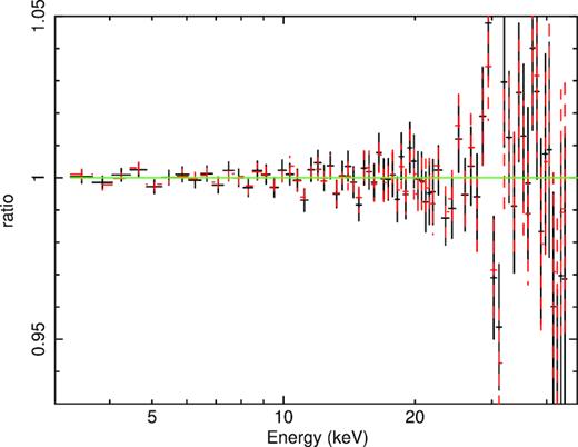
The data-to-model ratios of the model of G15 fitted to the data sets G (black solid crosses; model 0) and A (red dashed crosses).
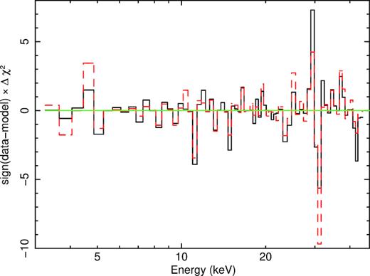
The contributions to χ2 of the model of G15 fitted to the data set G (black solid histogram; model 0) and A (red dashed histogram).
We then fit data set A, for which the results are only slightly different. We find |$R_{\rm in}\approx 14^{+2}_{-3}R_{\rm ISCO}$|, |$i\approx 31_{-2}^{+2^\circ }$|, |$Z_{\rm Fe}\approx 4.1^{+5.9}_{-1.0}$|, |$\log _{10}\xi \approx 3.4_{-0.2}^{+0.3}$|, |$\chi ^2_\nu \approx 64.8/61$|, and other parameters similar to those found for data set G. As we can see as in Fig. 3, the model-to-data ratios for data sets G and A are very similar. The inner radius is compatible with being within 2RISCO. For this data set, removing the absorption line results in only a slight increase in χ2, by +1.7. Given the similarity of the two spectra, we hereafter follow G15 and use only data set (G) obtained with their method. We note that our finding of similar-quality fits with both methods differs from that of G15, who found their fit to a summed spectrum to yield a much larger χ2 than that using their method.
We then consider the effect of Comptonization of the reflection component. In the coronal geometry, some of the reflected emission will pass through the corona and be scattered in it. This effect has been considered by S17 using the model simplcut.4 The main parameter of it is the scattering fraction, fsc, which is the fraction of the reflected photons that are Compton scattered in the corona, with 1 − fsc reaching the observer unmodified. Then, the scattered part of the spectrum is split between parts leaving the source and hitting the disc (where photons are removed from the model), as given by the reflection-fraction parameter of simplcut. In order to account for up- and down-scattering of photons out of the energy range of the PCA detector, we have extended the range of the photon energy used to calculate the models to 0.1–1000 keV with 2000 logarithmically spaced bins. In that model, there are two options for the scattering kernel. In one, photons are scattered into an e-folded power-law distribution (with the kernel given by equation 1 of S17), the same as the incident spectrum of relxill (see above). In the other, the Compton scattering model nthcomp (Zdziarski, Johnson & Magdziarz 1996) is used.
In S17, the former kernel was used for consistency with the assumption that the incident spectrum is an e-folded power law. Those authors also replaced the incident spectrum of relxill by simplcut(ezdiskbb), where ezdiskbb is a multicolour disc blackbody model allowing for a disc truncation (Zimmerman et al. 2005). The resulting spectrum differs from an e-folded power law only at low energies, where the contribution of the disc blackbody is substantial. However, our data set does not show any soft excess and we have opted to keep the e-folded power law as the incident spectrum (and keep |$\cal {R}$|, Γ, and Ecut equal to those fitted in relxill). This is also consistent with the calculations of the reflection in relxill. Thus, our model has the form tbabs[cutoffpl+simplcut(relxill)+xillver]gabs, where the relxill component gives now only the spectrum reflected by the e-folded power law. We have applied this model to the data set G. We have found that the best-fitting scattering fraction is null, and fsc = 0+0.27. Thus, Comptonization of reflection does not improve the fit and does not produce significant changes to the best-fitting parameters of the model of G15 as applied to the present data set and using the current version of relxill.
3.4 Models with relxill and a single Fe abundance
Now, we tie the Fe abundance for the static and relativistic reflection components and allow the former to be ionized. With this change, we find that the models no longer require the additional absorption line at 7.2 keV. Thus, our model has the form of tbabs(relxill+xillver). We find good fits with two kinds of models. In one, the blurred reflector is strongly ionized while the distant one is close to neutral, which is similar to the original model of G15 except for their assumptions of the separate Fe abundances and the presence of the absorption line. In the other, the blurred reflector is close to neutral while the distant one is strongly ionized. We note that both models have the same form, as given above. Thus, they actually represent two local minima of the same model. However, since their physical configurations are different while the χ2 values are similar, we consider them separately.
In the first model, we obtain a somewhat worse fit than that in Section 3.3, |$\chi _\nu ^2=68.7/61$|, and obtain |$R_{\rm in}\approx 19^{+33}_{-6}R_{\rm ISCO}$| and |$Z_{\rm Fe}\approx 3.1^{+2.0}_{-0.3}$|. For the second model, |$\chi _\nu ^2=68.3/61$|, and |$R_{\rm in}\approx 53^{+\infty }_{-26}R_{\rm ISCO}$|, |$Z_{\rm Fe}\approx 2.4^{+0.3}_{-0.2}$|; see models 1 and 2, respectively, in Table 1. Hereafter, we use the symbol ∞ to denote that the upper limit of Rin is approaching Rout. We note that the ionization parameter of the low-ionization disc part is very weakly constrained, and allowing it to be free only marginally improves the fit. Still, here and in most of the following models, we have opted not to freeze it at ξ = 1 in order to show the range allowed by the data. The contributions to χ2 from the two models are shown in Fig. 5. We see that while the values of χ2 for these models are somewhat higher than those in Section 3.3, the differences in their contributions per energy channel are very minor. We note that now the Fe abundances have lower, and much more likely, values than in the original model of G15. Also, both of our models give large truncation radii. The two models have the parameters relatively similar to each other except for the interchanged ionization parameters. This is possible because of the large fitted truncation radii, implying that the relativistic broadening is modest. There is also some difference in the strength of the reflection components. In the first model, the distant reflection component has a flux at 30 keV of about half of the flux in the relativistic component, while in the second model both reflection components’ fluxes become very similar at high energies.
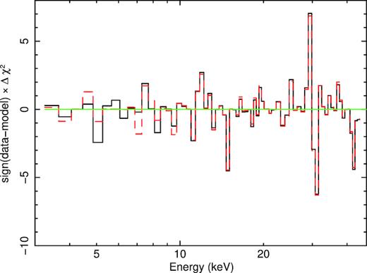
The contributions to χ2 of the relxill-type models with exponential cut-off. The black solid and red dashed histograms correspond to the models with the high (model 1) and low (model 2) ionization, respectively, of the close, relativistically-broadened, reflector. The vertical scales are the same as in Fig. 4.
We then consider the effect of the electron density of the reflector. In xillver, ne = 1015 cm−3 is assumed, which is likely to be too low for accretion discs in BH binaries. The effect of the value of ne on the reflection spectra was investigated by García et al. (2016). They pointed out an increase in thermal emission at low energies for a given value of ξ (since then the irradiating flux is then ∝ne and the effective temperature is |$\propto n_{\rm e}^{1/4}$|), which should not affect our results obtained at ≥3 keV. Also, the reflector temperature increases, which results in a higher ionization state. Currently, there are available models with ne up to 1019 cm−3, namely xillverD and relxillD (García et al. 2016), while models for higher ne are under development (García et al. 2018). Those two models assume that the e-folding energy is fixed at 300 keV, which is within the 90 per cent confidence regime of our models 1 and 2. Thus, we fit that model to the data. We consider only the case with low ionization of the remote reflector. The fit results for this model, #3, are given in Table 1. With respect to the corresponding model 1, we find a larger disc truncation radius, |$R_{\rm in}\approx 55_{-34}^{+\infty } R_{\rm ISCO}$|, and a higher Fe abundance, |$Z_{\rm Fe}\approx 4.9_{-0.9}^{+4.1}$|. The fit has a higher value of |$\chi _\nu ^2\approx 72.4/62$|, which appears to be mostly due to the fixed value of Ecut. We discuss these results in the context of other similar studies in Section 4.
We have then included Compton scattering of the reflected emission in the same way as in Section 3.3. We have found that in all three cases the best-fitting scattering fraction was zero (see Table 1).
3.5 Models with reflkerrExp (incident e-folded power law)
We now consider models of Niedźwiecki et al. (2019). The differences of these models with respect to relxill are described in detail in that paper. One difference is that the relxill assumes the incident spectra to have the high-energy cut-off (or temperature) constant with the disc radius in the observer’s frame, i.e. the incident spectra in the local frames are blueshifted with respect to that given as the model cut-off by 1 + z(r). On the other hand, reflkerr (Niedźwiecki et al. 2019) assumes the incident spectrum to be constant with radius in the local frames, i.e. the observed spectrum is the sum of the local spectra redshifted by 1 + z(r). Also, reflection in the reflkerr model merges the detailed photoionization calculations of xillver at low energies with the relativistically correct treatment of ireflect (Magdziarz & Zdziarski 1995) at high energies.
We first consider models with incident power-law spectra with exponential cut-offs. The model is then tbabs(reflkerrExp+hreflectExp), where reflkerrExp includes relativistic broadening, and hreflectExp is the corresponding static model. Similar to our results in Section 3.4, we find two possible models, with interchanged ionization parameter. In the model with high ionization of the blurred reflector, we obtain a fit with |$\chi _\nu ^2\approx 69.1/61$|. We find |$R_{\rm in}\approx 15^{+31}_{-12}R_{\rm ISCO}$|, |$Z_{\rm Fe}\approx 3.9^{+0.8}_{-1.4}$|; see model 4 in Table 1. The distant reflection component contributes about half of the flux of the relativistic one at 30 keV. The bolometric flux of this model is ≈2.6 × 10⁻⁸ erg cm−2 s−1, corresponding to a luminosity of |$L\approx 2.0\times 10^{38}(D/8\, {\rm kpc})^2$| erg s−1, and |$L/L_{\rm E}\approx 0.17(D/8\, {\rm kpc})^2 (M/8\, {\rm M}_{\odot })^{-1}$|.
For the model with low ionization of the close reflector, we find |$\chi _\nu ^2\approx 69.2/61$|, |$R_{\rm in}\approx 58^{+\infty }_{-28}R_{\rm ISCO}$|, and |$Z_{\rm Fe}\approx 2.6^{+0.6}_{-0.4}$| (see model 5 in Table 1). Both reflection components become almost identical at high energies. Taking into account Comptonization of the reflected radiation does not improve the fit in both cases (see the values of fsc in Table 1).
We can see a very good agreement between the results obtained with the current version (1.2.0) of relxill and with reflkerrExp. The two sets of models have almost identical parameters and the values of χ2; compare models 1 and 2 with models 4 and 5, respectively, in Table 1.
3.6 Models with reflkerr (incident thermal Comptonization)
We then consider models of Niedźwiecki et al. (2019) with the incident spectrum described by the thermal Comptonization, for which they use the model compps of Poutanen & Svensson (1996). Our present model has the form of tbabs(reflkerr+hreflect). For the model with high ionization of the close reflector, we find |$\chi _\nu ^2\approx 62.1/61$|, |$R_{\rm in}\approx 47^{+\infty }_{-45}R_{\rm ISCO}$| (with the lower 90 per cent confidence limit at Rin ≈ 1.8RISCO ≈ 2.2Rg) and |$Z_{\rm Fe}\approx 3.3^{+1.7}_{-1.0}$| (see model 6 in Table 1). The temperature of the Comptonizing medium is |$kT_{\rm e}\approx 20^{+3}_{-2}$| keV, and the temperature of blackbody seed photons is |$kT_{\rm bb}\approx 0.34^{+0.04}_{-0.09}$| keV. The Compton parameter, y ≡ 4(kTe/mec2)τT, where τT is the Thomson optical depth of the slab (approximating the corona), is |$y\approx 1.19^{+0.05}_{-0.08}$|. The distant reflection contributes about two-thirds of the flux of the relativistic one at 30 keV. In this model, in order to directly compare it to the model of G15, we have kept the ionization parameter fixed at ξ = 1. If we allow it to be free, log10ξ ≈ 0+1.9. The unfolded spectrum and the model are shown in Fig. 6 and the χ2 contributions are shown in Fig. 7.
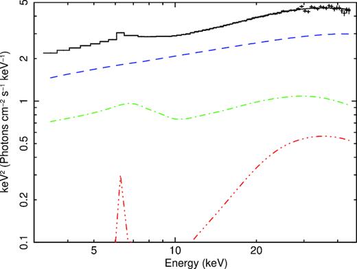
The histogram shows the unfolded spectrum (for model 6) as fitted by thermal Comptonization (dashed blue curve) and two reflectors, an inner highly ionized one (dot–dashed green curve), and an outer weakly ionized one (triple dot–dashed red curve). The solid curve gives the total model.
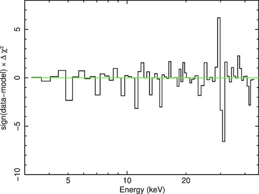
The contributions to χ2 of the reflkerr model (#6) with the incident spectrum due to thermal Comptonization and high ionization of the relativistically broadened reflector. The vertical scales are the same as in Fig. 4.
The posterior probability distributions and correlations between the parameters obtained using the MCMC technique (see Section 3.1) are shown in Fig. 8, obtained using the package of Foreman-Mackey (2016). We see here rather wide probability distributions of Rin, which, however, become very small for |$R_{\rm in}\lesssim 10 R_{\rm ISCO}$|. The strongest correlations include the positive ones between ξ(inner), ZFe and y. Also, there is some positive correlation between |$\cal {R}$|(inner) and the inclination. Overall, we see that this model has its parameters relatively well constrained, except for the relatively wide allowed range of Rin.
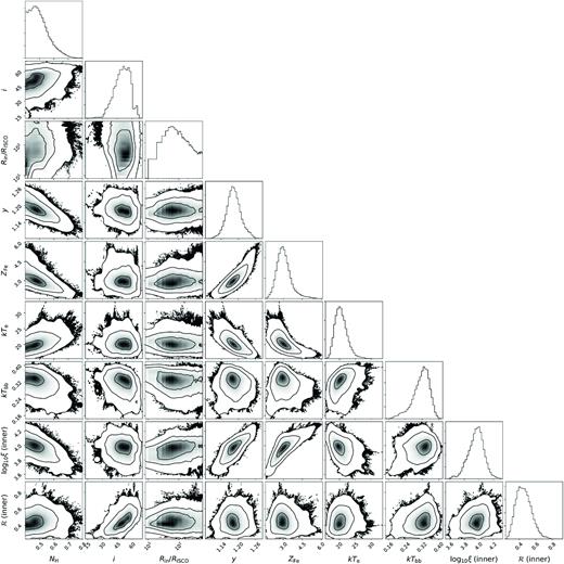
The posterior probability distributions (proportional to the relative frequency of the fitted models) showing correlations between pairs of the parameters of the reflkerr model (#6), obtained using the MCMC method. The inner, middle, and outer contours correspond to the 2D significance of σ = 1, 2, 3, respectively, also shown by the degree of the darkness. The rightmost panels show the probability distributions for the individual parameters (with the normalization corresponding to the unity integrated probability). See Section 3.6 for discussion.
Including Comptonization of reflection very slightly reduces the value of χ2, to |$\chi _\nu ^2\approx 62.0/60$|, at |$f_{\rm sc}\approx 0.30_{-0.30}^{+0.15}$|, and yields very similar other parameters. The relatively low value of fsc can be reconciled with the relatively large τT of the model in the geometry of a central hot flow surrounded by a truncated disc, in which relatively few reflected photons return into the hot flow (see e.g. Zdziarski, Lubiński & Smith 1999; Poutanen, Veledina & Zdziarski 2018).
S17 also considered models without the presence of a distant reflector. Here, we confirm their conclusion that such models give a much worse description of the data using our model 6. If we do not include the static reflection component, we obtain Δχ2 ≃ +22 for one less d.o.f., which corresponds to the probability of the fit improvement by adding that component being by chance of 2 × 10⁻⁵ (using the F-test).
In the case with low ionization of the close reflector, we also find a very good model, for which |$\chi _\nu ^2\approx 63.8/60$|, |$R_{\rm in}\approx 100^{+\infty }_{-62}R_{\rm ISCO}$|, |$Z_{\rm Fe}\approx 2.9^{+0.5}_{-0.3}$|, and |$i\approx 18^{+57^\circ}_{-6 }$|. The high-ionization, distant reflection actually dominates in this model, with its flux at 30 keV being higher by ≈1.7 than that of the close reflection. Including Comptonization of reflection (using simplcut with the nthcomp scattering kernel) improves the fit only marginally. For the sake of the simplicity of the presentation, this model is not included in Table 1.
4 DISCUSSION AND CONCLUSIONS
Our main finding is that X-ray spectra of the hard state of GX 339–4 from the PCA can be fitted with similar statistical quality with models allowing significantly different disc truncation radii, namely with Rin either close to or much larger than RISCO. Still, all of the fitted models prefer the latter at their best-fitting values. This is the case (Rin ≈ 11RISCO) even for the original model (#0 in Table 1) of G15 fitted to our average PCA spectrum with the current version of the relxill software. That model, however, requires the presence of a 7.2 keV absorption line, separate Fe abundances for the two reflectors, and a high value of the Fe abundance for the relativistic reflector.
While the presence of an absorption line at 7.2 keV is in principle possible, it has not been found in other observations of GX 339–4. In systematic studies of BH X-ray binaries, GX 339–4 shows the same properties as systems without disc-wind absorption lines. In particular, the shape of the track on the hardness-count rate diagram of GX 339–4 favours a relatively low inclination (Muñoz-Darias et al. 2013). Also, high-ionization Fe K absorption lines in the soft state, which trace disc winds, have not been detected in GX 339–4 (Ponti et al. 2012). Then, while the assumption of strongly different Fe abundances in the two reflectors can be motivated by our lack of knowledge of the true model of the accretion flow, it does not have a direct physical interpretation.
On the other hand, we have found alternative models (#1–6 in Table 1), which rule out Rin ≈ RISCO at 90 per cent confidence. In particular, if we impose a common Fe abundance in both reflection components and keep the assumption of the exponential cut-off of the incident spectrum (models 1–5), we find |$R_{\rm in}\gtrsim 6 R_{\rm ISCO}$|, using either relxill or reflkerrExp. The models no longer require the 7.2 keV absorption line and their fitted Fe abundances are relatively moderate, |$Z_{\rm Fe}\gtrsim 2$|. Still, they have somewhat higher value of χ2 than the model following the assumptions of G15, with Δχ2 ≈ 2–3. Also, those models in the variant with high ionization of the close reflector (#1, 3, 4, which appear more likely; see below) yield the disc inclinations close to face-on, which are only marginally consistent with the constraint on the binary inclination of 37° ≤ ib ≤ 78° (Heida et al. 2017). Since those models imply the presence of a truncated disc with Rin ≫ RISCO, the disc axis is likely to be aligned with the binary axis rather than the BH spin axis. We note that S17 argued that disc truncation in GX 339–4 requires a highly super-Eddington accretion rate. However, that argument is incorrect since it considers only the viscously generated soft seed photons but neglects the abundant soft photons from reprocessing of the hot-flow emission in the irradiated disc, as discussed in detail in Poutanen et al. (2018). Both the viscously generated photons and those due to re-emission of the irradiating flux absorbed in the disc form then a soft quasi-blackbody spectral component around the disc inner radius. This component corresponds to the blackbody seed photons in model 6.
Our overall best-fitting model (#6 in Table 1), with the lowest value of |$\chi _\nu ^2\approx 62/61$| and the by far highest Akaike likelihood, has a physical thermal-Comptonization primary continuum rather than a phenomenological e-folded power law. The best-fitting value of the truncation radius is several tens of RISCO, and |$R_{\rm in}\gtrsim 2 R_{\rm ISCO}$| within the 90 per cent confidence limits. The Fe abundance is the same for both reflectors, and moderate, ZFe ≈ 3, and there is no absorption line at 7.2 keV required. This model also has the best-fitting inclination, |$i\approx 49^{+34}_{-26^ \circ }$|, in good agreement with the constraint of Heida et al. (2017). We stress this is the only model among those considered that has a moderate Fe abundance, an inclination in agreement with that measured for the binary and the ionization of the distant reflection lower than that of the inner disc (which appears more likely; see below). On the other hand, only some, but not all, of those desired features appear in other models considered.
The primary continuum in this thermal-Comptonization model differs quite significantly from an e-folded power law at high energies. The difference between the two types of spectra is illustrated, e.g. in fig. 5(b) of Zdziarski et al. (2003). The Comptonization spectrum in that case has kTe = 25 keV, close to our best-fitting value of |$20^{+3}_{-2}$| keV. We see in that figure that the Comptonization spectrum has an approximately single power-law shape up to ≈50 keV, and then it shows a sharp cut-off. On the other hand, an e-folded power law features a gradual attenuation, visible already at E ≪ Ecut. In the example shown in Zdziarski et al. (2003), an e-folded power law with Ecut = 150 keV lies below the Comptonization spectrum already by |$E\gtrsim 10$| keV. This effect explains the mismatch between the values of kTe and Ecut that we found, with Ecut ≫ kTe fitted here to the same spectrum at E ≤ 45 keV.
For all of our models, we have also taken into account Comptonization of the reflected component. However, we have found this effect to be minor. In model 0 (which follows the assumptions of G15), the reflection fraction is |${\cal R}\approx 0.06$| and the fraction of the reflection photons scattered in the corona is |$\lesssim 0.3$|; such values rule out a corona above a disc extending to the ISCO. On the other hand, the relatively low values of |$\cal R$| in our other models are consistent with truncation and the primary continuum originating partly in a corona and partly in a hot flow at R < Rin (Zdziarski et al. 1999). Our physical (and statistically best) thermal Comptonization model is also compatible with the energy balance constraint (see e.g. the recent study of Poutanen et al. 2018).
We have also investigated the effect of increasing the reflector density. Using the model of García et al. (2016) with ne = 1019 cm−3 (#3 in Table 1), we have found an increase of both the truncation radius and the Fe abundance with respect to the corresponding model with an exponential cut-off and ne = 1015 cm−3. In particular, ZFe increased from ≈3 to ≈5 at the best fit.
The increase in ZFe we found is surprising, given the results of Tomsick et al. (2018). They have studied the effect of changing the reflector density for the case of a hard/intermediate spectrum of Cyg X-1 from Suzaku and NuSTAR. In the case of free Fe abundance, coronal geometry, and ne = 1015 cm−3, they obtained, using relxill+xillver, an extreme abundance of ZFe ∼10 and a very low disc inner radius of |$R_{\rm in}=1.33_{-0.06}^{+0.03} R_{\rm ISCO}$|. Then, they used the reflection model reflionx_hd of Ross & Fabian (2007), which assumes ZFe = 1 but allows for a free reflector density. The best fit in that case was obtained for ne ≈ 4 × 1020 cm−3, a much larger truncation radius, |$R_{\rm in}\approx 7.3_{-1.9}^{+4.6} R_{\rm ISCO}$|, and at a much lower value of χ2 than in the previous case. Thus, the effects of allowing a high density in that case are an increase of the truncation radius and obtaining a good fit at the solar Fe abundance. While the former is in agreement with our finding, the latter effect is opposite. The reason for this disagreement is unclear; it may be related to a difference in the treatment of atomic processes in the reflecting/reprocessing medium between the reflionx_hd and relxill models.
We note that the actual characteristic value of ne of the reflecting medium is uncertain. García et al. (2016) estimated it using the radiation-pressure dominated disc solution including the effect of coronal dissipation of Svensson & Zdziarski (1994). However, this density is averaged over the disc height, and it is close to that in the disc mid-plane. The corresponding Thomson optical depth of that solution is ≫10, and the reflecting surface layer has an optical depth of several and a much lower average density, given by the vertical hydrostatic equilibrium. Furthermore, the actual density is a function of both the radius and the depth within the disc.
A possible check on the self-consistency of an approximate solution is using the definition of ξ (equation 3). The irradiating flux in a coronal geometry can be expressed as the ratio of the luminosity to the emitting area, where the latter can be estimated as |$x R_{\rm in}^2$|, where the constant x ∼ 1 expresses our (large) uncertainty about the area. In the case of Cyg X-1, L ≈ 1.8 × 1037 erg s−1, Rin ∼ 10Rg (Tomsick et al. 2018) and M ≈ 15M|$\odot$| (Orosz et al. 2011). The fitted ionization parameter was ξ ≈ 2000 erg cm−2 s−1, which implies ne ≈ (2/x) × 1020 cm−3, rather close to the density fitted in that work. In the case of our observation of GX 339–4 and model 3, L ≈ 2 × 1038 erg s−1, ξ ≈ 5000 erg cm−2 s−1, Rin ∼ 50RISCO, which yields ne ≈ (2/x) × 1019 cm−3. This implies that only model 3 can be considered as approximately self-consistent. However, given that the current version of the xillverD model allows for only for one option of the high-energy cut-off, we could not consider other options with it, in particular that with a thermal Comptonization primary spectrum.
In our analysis, we found that the data allow the ionization of the outer reflector to be higher than the inner one. This effect is due to the relatively modest relativistic effects in the inner reflector, which then allows for its interchange with the outer, static, one. Since ξ∝Firr/ne, it is not a priori obvious that the surface layers of the outer disc are weakly ionized, given that they are irradiated by the strong X-ray emission from the central source, with the disc likely to be flared. Still, those solutions (#2, 5 in Table 1) appear less likely. We give them for the sake of the completeness of the presentation of our analysis results.
We stress that our most physically motivated case uses a one-zone thermal Comptonization model. In the case of the hard state of the BH binary Cyg X-1, Axelsson & Done (2018) found that the X-ray variability properties require the presence of three separate Comptonization components with different spectral slopes and temperatures. Yamada et al. (2013) obtained a similar conclusion from analysing the broad-band variability in Cyg X-1. Mahmoud & Done (2018a,b) modelled the spectral and timing properties of Cyg X-1, finding that rather complex models are required. In GX 339–4, observational evidence for two Comptonization zones has been recently reported from the full spectral-timing modelling of one XMM–Newton hard-state observation of the source (Mahmoud et al. 2018). Given that result and the overall similarity of the spectral and timing properties of Cyg X-1 and GX 339–4, our one-zone Comptonization modelling appears to be too simple to describe the actual accretion flow. However, since the RXTE data studied here cover the range of |$\ga$|3 keV only, the second, soft, Comptonization component in the model of Mahmoud et al. (2018, see their fig. 4) contributes negligibly to the range fitted by us, and it does not affect the validity of our results.
We can compare our models to those that Basak & Zdziarski (2016) fitted to their EPIC-pn spectrum 7, in particular for their model 2(ii), which includes a static reflection component. That fit yields |$R_{\rm in}=19.5^{+15.0}_{-8.0}R_{\rm g}$| and |$\Gamma \approx 1.67^{+0.02}_{-0.02}$|, which are compatible with our results. The main differences are the high ionization of the outer static reflector, about the same as that of the inner one, and the Fe abundance, which they find to be about solar, with |$Z_{\rm Fe}=0.95^{+0.07}_{-0.06}$|. Basak & Zdziarski (2016) also fitted a simultaneous PCA spectrum, and noticed a mismatch between the EPIC-pn and PCA calibration in the Fe K region (see their fig. 8).
We note that a PCA spectrum of GX 339–4 in the hard spectral state has been used to test an alternative GR theory as well as to measure the BH spin (Wang-Ji et al. 2018a), assuming that the disc extends to the ISCO (see their table II). In light of our results, that test appears to be highly uncertain.
We stress that we have found a very good agreement between the models using the present version of relxill and reflkerrExp. They yield almost identical values of Rin and other parameters at very similar χ2 (see Table 1).
Concluding, our spectral fitting results support the truncated disc paradigm for the hard state (Done et al. 2007), but allow the reflecting disc to extend to within about two ISCO radii within the 90 per cent confidence limit. Still, our results are based on a single spectrum (though with a very large count number of 107). Stronger constraints can be obtained while simultaneously fitting several data sets (as G15 did for their particular model).
ACKNOWLEDGEMENTS
We thank the referee for valuable comments, Javier García for discussions and explanations regarding the spectral analysis performed in G15, Jorge Casares and Jean-Pierre Lasota for discussions about disc inner radii in the quiescent state, Piotr Lubiński for discussion about the Akaike formalism, and Michael Parker for advice on the MCMC plotting. AGM acknowledges partial funding from NCN grant 2016/23/B/ST9/03123. This research has been supported in part by Polish National Science Centre grants 2013/10/M/ST9/00729, 2015/18/A/ST9/00746, 2016/21/B/ST9/02388, and 2016/21/P/ST9/04025.
Footnotes
As described in the RXTE data reduction cookbook: http://heasarc.nasa.gov/docs/xte/recipes/cook_book.html.
