


Abstract
We use the MusE GAs FLOw and Wind (MEGAFLOW) survey to study the kinematics of extended disc-like structures of cold gas around z ≈ 1 star-forming galaxies. The combination of VLT/MUSE and VLT/UVES observations allows us to connect the kinematics of the gas measured through Mg ii quasar absorption spectroscopy to the kinematics and orientation of the associated galaxies constrained through integral field spectroscopy. Confirming previous results, we find that the galaxy–absorber pairs of the MEGAFLOW survey follow a strong bimodal distribution, consistent with a picture of Mg ii absorption being predominantly present in outflow cones and extended disc-like structures. This allows us to select a bona-fide sample of galaxy–absorber pairs probing these discs for impact paramometers of |$10{-}70\,\, {kpc}$|. We test the hypothesis that the disc-like gas is co-rotating with the galaxy discs, and find that for seven out of nine pairs the absorption velocity shares the sign of the disc velocity, disfavouring random orbits. We further show that the data are roughly consistent with inflow velocities and angular momenta predicted by simulations, and that the corresponding mass accretion rates are sufficient to balance the star formation rates.
1 INTRODUCTION
A number of arguments (theoretical and observational) indicate that galaxies cannot be closed boxes with an ab-initio fixed reservoir of gas. Indeed, numerical simulations show that galaxies grow from the accretion of cool intergalactic gas (via the cosmic web), a process most efficient in galaxies with luminosities lower than L* (White & Frenk 1991; Birnboim & Dekel 2003; Kereš et al. 2005; Dekel & Birnboim 2006; Dekel et al. 2009; van de Voort et al. 2011; L’Huillier, Combes & Semelin 2012) owing to the short cooling times in these haloes (Rees & Ostriker 1977; Silk 1977). Observationally, a number of indirect arguments support the notion that galaxies need to continuously replenish their gas, implying that they are continuously fed by the accretion of gas from the intergalactic medium (IGM), as reviewed in Fox & Davé (2017).
Originally, the most common indirect argument comes from the G-dwarf problem (van den Bergh 1962; Schmidt 1963), which says that the metallicity distribution of G stars in the solar neighbourhood is not consistent with the closed-box expectations, and the data can be reconciled with chemical models provided that there is a significant amount of metal-poor infall (Larson 1972a,b; Lynden-Bell 1975; Pagel & Patchett 1975; Casuso & Beckman 2004). Another common indirect argument relies on the observed short gas depletion time-scales (≡Mgas/SFR), seen in local and distant galaxies to be typically 0.5–2 Gyr (e.g. Daddi et al. 2010; Tacconi et al. 2010, 2013, 2018; Freundlich et al. 2013; Saintonge et al. 2013, 2016, 2017; Genzel et al. 2015; Schinnerer et al. 2016; Scoville et al. 2016, 2017). These short depletion times imply that the observed amount of gas available is too low to sustain their star formation rate (SFR) for more than a few Gyr, i.e. it is not enough to support the galaxies’ future star formation. A third indirect argument comes from the slow decline of the cosmic H i density as a function of redshift (e.g. Péroux et al. 2003; Neeleman et al. 2016) tied to the gas content of galaxies (Wong & Blitz 2002).
As mentioned, in low-mass galaxies hosted by haloes below the virial shock mass threshold (|$M_{h} \lesssim 10^{11-12} \, \mathrm{M}_\odot$|) gas accretion is expected to be very efficient (e.g. White & Frenk 1991; Birnboim & Dekel 2003; Kereš et al. 2005; Faucher-Giguère, Kereš & Ma 2011; Nelson et al. 2015; Correa et al. 2018). Once inside the galaxy dark matter halo, the accreted gas is expected to orbit the galaxy, bringing along not only just fuel for star formation but also angular momentum (e.g. Stewart et al. 2011b, 2013, 2017; Danovich et al. 2015). In this context, the accreting material coming from the large-scale filamentary structure should form a warped, extended gaseous structure (e.g. Kimm et al. 2011; Pichon et al. 2011; Shen et al. 2013; Danovich et al. 2015; Stewart et al. 2017), which co-rotates with the central disc and is sometimes referred to as a ‘cold-flow disc’ (Stewart et al. 2011b, 2013, 2017).
This ‘cold-flow disc’ scenario leads to large gaseous (T ∼ 104 K) structures, which could in part become the large discs often seen around galaxies in H i 21cm surveys and extending 2–3 times beyond the stellar radius (e.g. Bosma 1981; Putman et al. 2009; Bigiel et al. 2010; Kreckel et al. 2011; Wang et al. 2016; Ianjamasimanana et al. 2018).
At higher redshifts, the ‘cold-flow disc’ scenario is expected to lead to distinct signatures in absorption systems with |$N_{{{\rm H\, \small {I}}}}$| of 1017–1021 cm−2 seen in background quasar sightlines (Dekel et al. 2009; Fumagalli et al. 2011; Kimm et al. 2011; Stewart et al. 2011a, 2013; Goerdt et al. 2012; van de Voort & Schaye 2012). In particular, some of the infalling gas kinematics is expected to be offset from the galaxy’s systemic velocity when observed in absorption along the sightlines of background quasars (Stewart et al. 2011a), because the gas is partly rotationally supported.
These expected signatures are testable against observations with suitably located background sources such as quasars (Barcons, Lanzettat & Webb 1995; Steidel et al. 2002; Chen, Kennicutt & Rauch 2005; Kacprzak et al. 2010, 2011; Bouché et al. 2013; Turner et al. 2014; Bouché et al. 2016; Ho et al. 2017; Rahmani et al. 2018), bright galaxies (Diamond-Stanic et al. 2016), or directly in redshifted absorption lines in galaxy spectra (down-the-barrel; Coil et al. 2011; Martin et al. 2012; Rubin et al. 2012; for review see Rubin 2017).
Among background sources, background galaxies are more numerous, but their usefulness is usually limited by the typically low S/N unless one reverts to a stacking approach as in Bordoloi et al. (2011). By contrast, background quasars are rarer, but allow one to obtain more informations, such as the gas location from the host, gas ionization properties (e.g. Muzahid et al. 2015; Lehner et al. 2016; Prochaska et al. 2017) and most importantly the gas kinematics (e.g. Barcons et al. 1995; Steidel et al. 2002; Kacprzak et al. 2010; Bouché et al. 2013, 2016; Ho et al. 2017). Among those, Ho et al. (2017) demonstrated the existence of co-rotating structures at z ≈ 0.2 in a sample of half-dozen galaxies, a step forward from the individual analyses of Bouché et al. (2013) and Bouché et al. (2016).
Progress in sample size has been slow in spite of decades of research with galaxy–quasar pairs, as studies investigating the connections between the host galaxy kinematics and the low-ionization absorption line kinematics were limited to ∼50 pairs (see Kacprzak 2017, for a recent review). Less than half of these have orientations favourable to study extended gas discs (accretion cases) (Barcons et al. 1995; Steidel et al. 2002; Chen et al. 2005; Kacprzak et al. 2010, 2011; Bouché et al. 2013, 2016; Ho et al. 2017; Rahmani et al. 2018).
Thanks to the MUSE (Multi Unit Spectroscopic Explorer; Bacon et al. 2006, 2010) instrument on the VLT (Very Large Telescope) with its unprecedented field-of-view (FoV) (1 × 1 arcmin) and sensitivity, the situation is about to change significantly by taking advantage of the combination of MUSE kinematics and high-resolution UVES (Ultraviolet and Visual Echelle Spectrograph; Dekker et al. 2000) data. Indeed, we recently started the MuseE GAs FLOw and Wind (MEGAFLOW) survey (Bouché et al. in preparation), which consists of MUSE + UVES observations of 22 quasar fields, each with multiple (three or more) strong (>0.5–0.8 Å) Mg ii absorbers at redshifts 0.3 < zabs < 1.5 selected from the JHU-SDSS catalogue (Zhu & Ménard 2013). The MEGAFLOW survey leads to one of the largest surveys of Mg ii absorber–galaxy pairs with spectroscopic and kinematic information, with about 80+ galaxy–quasar pairs suitable to study either outflows (as in Schroetter et al. 2016; hereafter Paper I) or accretion (as in Bouché et al. 2016, this work) depending on the apparent location of the quasar with respect to the galaxy major-axis.
In this paper, we present results on nine galaxy–quasar pairs suitable for characterizing the kinematics of accreting gas, while the wind cases will be presented in a companion paper (Schroetter et al. in preparation). After briefly introducing the MEGAFLOW survey (Section 2), we discuss in Section 3 the observation and reduction strategy both for the MUSE and UVES data. The selection of the nine galaxy–quasar pairs of this study from the ≈80 absorbers pairs in the MEGAFLOW survey is discussed in Section 4. Then, we infer kinematical and physical properties of the selected galaxies and their host haloes in Section 5. As the main result of our work, we compare galaxy to absorber kinematics in Section 6, with a focus on testing for co-rotation and potential radial infall.
Throughout this paper, we use the Lambda cold dark matter standard cosmological parameters: H0 = 70 km s−1, ΩΛ = 0.7, and Ωm = 0.3. All distances are proper. Further, we assume a Chabrier (2003) stellar initial mass function (IMF) and all stated magnitudes are on the AB system (Oke 1974). When we refer in the following to [O ii] without additional wavelength qualifier, we refer to the [O ii] λλ3727, 3729 doublet. The prefix ‘pseudo’ in pseudo-filter and pseudo-spectrum refers to the fact that these were created from the MUSE data cube. All stated uncertainties are 68 per cent confidence intervals. The nine galaxy–absorber pairs can be identified throughout by uniquely assigned colours.
2 THE MEGAFLOW SURVEY
2.1 Motivation
Since the initial work of Bergeron (1988), Bergeron & Boissé (1991), Steidel (1995), and Steidel et al. (2002), there is a well-established association between the cool (T ∼ 104 K) component of the CGM traced by the low-ionization Mg ii doublet seen in absorption in background quasar spectra and star-forming galaxies. Large samples of galaxy–quasar pairs are rare and difficult to construct owing to the difficulty in finding the host galaxy responsible for the Mg ii absorption, which is often a painstaking process requiring deep imaging (preferably from the Hubble Space Telescope) and multi-object spectroscopy, with the added problems of the quasar point spread function (PSF) blocking the view directly along the line of sight (LOS). One of the largest samples of Mg ii selected galaxy–quasar pairs with morphological data is the MAGIICAT sample (Churchill et al. 2013; Nielsen et al. 2013a; Nielsen, Churchill & Kacprzak 2013b; Nielsen et al. 2015, 2016), which consists of 123 isolated foreground galaxies with associated Mg ii detections at 0.07 ≤ z ≤ 1.1.
Surveys of galaxy–quasar pairs such as the MAGIICAT sample suffer from two major limitations, namely that they must rely on photometric pre-selection (i.e. suffer from redshift incompleteness) and that they lack kinematical information on the host galaxies. Both of these limitations must be overcome using expensive follow-up spectroscopic campaigns. This can be partially by-passed with integral field unit (IFU) surveys as described in Bouché (2017) because IFU surveys can simultaneously (i) locate the host galaxy; (ii) determine the host photometric and kinematics properties; (iii) determine the host morphological properties in most cases; and (iv) allow for proper PSF subtraction in case of small impact parameters.
2.2 The survey
With the FoV (1 × 1 arcmin), sensitivity, and wavelength coverage of the VLT/MUSE instrument (|${\sim }4800\,{-}9300\, {\mathring{\rm A} }$|), building large samples of absorber–galaxy pairs is now feasible with only a handful of observing nights. In particular, we started the MEGAFLOW survey of 22 quasar fields, which aims at building a sample of ∼100 galaxy–quasar pairs. In order to reach this goal, we selected quasars from the JHU-SDSS Mg ii absorber catalogue (Zhu & Ménard 2013) which had at least three (or more) Mg ii absorbers within the redshift range from 0.4 to 1.5, suitable for [O ii] based identification of star-forming galaxies in the MUSE wavelength range.1 In addition, we imposed that the rest-frame equivalent width of |${{\rm Mg}\, \rm \small {II}}\, \lambda 2796$|, |$\mathrm{ EW}_0^{\lambda 2796}$|, of the three required absorbers be greater than |$0.5\, \mathrm{\mathring{\rm A} }$|, with a preference given to sightlines with multiple |${\mathrm{ EW}_0^{\lambda 2796}}\,\gt \,0.8\, \mathrm{\mathring{\rm A} }$| absorbers. The restriction on Mg ii rest equivalent width |${\mathrm{ EW}_0^{\lambda 2796}}\,\gt\, 0.5\, \mathrm{\mathring{\rm A} }$| was chosen because the host galaxy is then expected to be within ≈100 kpc of the quasar LOS, i.e. matching the field of view of MUSE, given the well-known anticorrelation between the impact parameter and |$\mathrm{ EW}_0^{\lambda 2796}$| (Lanzetta & Bowen 1990; Bergeron & Boissé 1991; Steidel 1995; Chen et al. 2010; Bordoloi et al. 2011; Nielsen et al. 2013a; Werk et al. 2013). A slightly less stringent equivalent width threshold of |${\mathrm{ EW}_0^{\lambda 2796}}\,\gt\, 0.3 {\mathring{\rm A} }$| is often used in the literature to separate strong Mg ii absorbers from weak Mg ii absorbers (e.g. Churchill et al. 1999). Our 22 quasar sightlines serendipitously include several (10) absorbers with |$0.3\, \mathrm{\mathring{\rm A} }\, \lt\, {\mathrm{ EW}_0^{\lambda 2796}}\,\lt\, 0.5\, \mathrm{\mathring{\rm A} }$| in the right redshift range. We included these absorbers in the analysis. Even so their equivalent widths are slightly below our survey threshold, the galaxy–absorber association for absorbers of this strength is still expected to be sufficiently robust. In total, the 22 quasar sightlines contain 79 strong |${{\rm Mg}\, \rm \small {II}}$| absorbers with |${\mathrm{ EW}_0^{\lambda 2796}}\,\gt\, 0.3\, \mathrm{\mathring{\rm A} }$| with 0.51 < z < 1.45.
3 DATA
Each quasar field was observed with MUSE and each quasar was followed up with the high-resolution spectrograph UVES at the VLT.
3.1 MUSE observations
We observed all 22 quasar fields with the VLT/MUSE instrument over the period 2014 September–2017 May2 as part of guaranteed time observations (GTO). A full description of the data for all 22 fields will be given in a future paper describing the full survey (Bouché et al., in preparation). Briefly, all except three fields were observed for at least 2 h, i.e. the resulting exposure times are |$\ge6\,\mathrm{ks}$|. Observation details are listed in Table 1.
Details of MUSE observations for the 22 MEGAFLOW quasar fields as used in this study. The full table with all 22 fields is in Table C1 of the Supplementary Appendix. (1) Quasar/field identifier; (2) right ascension of the QSO [hh:mm:ss; J2000]; (3) declination of the QSO [dd:mm:ss; J2000]; (4) total MUSE exposure time (ks); (5) seeing full width at half maximum (FWHM) measured at 7050 Å by fitting a Gaussian (arcsec); (6) seeing FWHM measured at 7050 Å by fitting a Moffat profile with β = 2.5 (arcsec); (7) date of observations; (8) ESO program IDs; (9) reference.
| MUSE observations | ||||||||
|---|---|---|---|---|---|---|---|---|
| Quasar | RA | Dec. | Texp | Seeing (G.) | Seeing (M.) | Date-Obs | Prog. IDs | Refs |
| (1) | (2) | (3) | (4) | (5) | (6) | (7) | (8) | (9) |
| J0145p1056 | 01:45:13.1 | +10:56:27 | 6.0 | 1.03 | 0.85 | 2015-11-12, | 096.A-0164(A), | This work |
| 2016-08-29 | 097.A-0138(A) | |||||||
3.1.1 Data reduction
We reduced the data using the ESO MUSE pipeline version v1.6 (Weilbacher et al. 2012, 2014; Weilbacher, Streicher & Palsa 2016). First, each individual exposure was processed by the scibasic recipe to produce a table (hereafter called pixtable) containing relative locations, wavelength, counts, and an estimate of the variance. This recipe removes the instrumental signatures by applying daily calibrations (lamp flat-fields, bias, twilight-flat illumination corrections) and calibrates the wavelength scale (based on daily arc-lamps). Further, scibasic also applies the geometric solution (determined once per GTO run) for each of the 24 IFUs. Bad pixels corresponding to known CCD defects (columns or pixels) are also masked at this time. For each exposure we also used an ‘illumination’ exposure, which are short flats, to correct for flux variations on the slices due to small temperature changes between the daily calibration exposures and the science exposures.
Secondly, the individual pixtables were flux-calibrated (using the response from daily standards), telluric corrected (using a telluric absorption estimate from the flux-standard), sky-subtracted, astrometrically calibrated, and resampled on to a cube (using the drizzle algorithm) with the pipeline’s scipost recipe. However, clear variations of the residual background level between individual slices were visible in white-light images created from the cube, caused by imperfections from the flat-fielding/illumination correction. To mitigate these imperfections we used a self-calibration strategy, as in Bacon et al. (2015, 2017), which is conceptually similar to the CubeFix method developed by Cantalupo (in preparation, see also Borisova et al. 2016 and Marino et al. 2018). Essentially, it consists of normalizing the background in all slices to the overall background level.
In practice,3 we were using the ‘self-calibrate’ method in the python package mpdaf (MUSE Python Data Analysis Framework) v2.3dev (Bacon et al. 2016, Piqueras et al. 2017). This method computes the multiplicative corrections necessary to bring each slice to the reference background level, which is determined by the mean sky background across the field. Consequently, it requires as input a ‘positioned’4 pixtable with the sky subtraction turned off, and an object mask. We used sextractor on the white light images (as described above) to produce the object masks and we reran the scipost from the 24 scibasic pixtables to produce a ‘positioned’ scipost pixtable per exposure. In this rerun of scipost, sky subtraction and correction for barycentric velocity were switched off. Because the self-calibration does successfully remove the slice-to-slice variations but fails to remove the sharp flat-field imperfections visible at the edges of the IFUs, we simply masked the affected regions in the scibasic pixtables used as input.
After performing the self-calibration, we resampled the corrected positioned pixtables to datacubes using again the scipost recipe. Here, we performed the sky subtraction, barycentric correction, and use the same 3D output world coordinate system (WCS) grid for each of the cubes. We then used the software-package Zurich Atmosphere Purge (zap) (Soto et al. 2016a,b) to remove skyline residuals from each datacube, which makes use of a principal component analysis PCA analysis using cftype=‘fit’ and using an improved object mask created from the white-light pseudo-images. After manual inspection of the individual cubes and masking of visible satellites tracks, we combined the cubes. For those fields where the seeing between individual exposures was strongly differing, we weighted each exposure with the inverse of the full width at half maximum (FWHM) of the PSF.
3.1.2 Data characterization
In order to assess the image quality, we measured the PSF on the quasar itself in the combined cubes by fitting an elliptical 2D Moffat profile (Moffat 1969). Due to the large wavelength range covered by the MUSE data (from 4800 to 9300 Å), we measured the PSF as a function of wavelength using |$100\, {\mathring{\rm A} }$| wide pseudo-filter images at five different wavelengths separated by |$1000\, {\mathring{\rm A} }$|, and interpolated these measurements for other wavelengths. We first performed the PSF measurement on each of these images using a Moffat profile with β set to 2.5. The Moffat FWHM values at |$7050\, {\mathring{\rm A} }$| range from 0|${^{\prime\prime}_{.}}$|53 to 0|${^{\prime\prime}_{.}}$|98 across the 22 fields, with a median value of 0|${^{\prime\prime}_{.}}$|76. Secondly, we also determined the wavelength dependence of the PSF with the pampelmuse code (Kamann, Wisotzki & Roth 2013) using a Moffat profile with the β parameter free. Overall, the difference between the fixed-β values and the free-β pampelmuse values are different by a median of 5 per cent and at most 14 per cent.
In order to obtain a realistic estimate for our sensitivity to [O ii] emitters, we estimated the 5σ point source detection limit in a pseudo-NB filter with an appropriate width of |$400\, {\rm km\,s^{-1}}$|. A filter width of |$400\, {\rm km\,s^{-1}}$| gives the optimal S/N for the |${[{\rm O}\, \rm \small {II}}]{}\, \lambda \lambda 3727,3729$| doublet when assuming a line width of |$\rm {FWHM}\approx 50\, {km\,\,s^{-1}}$|. In the spatial direction, we assumed a circular detection aperture with radius of 1.5 × FWHMMoffat. This aperture size gives the optimal S/N for a point source convolved with a Moffat PSF with β = 2.5 in the background limited case. By using an estimate for the per-pixel noise and scaling it to the number of pixels spanned by the assumed spatial size and filter width, we derived an estimate for the total noise within the aperture. Subsequently, we multiplied this noise estimate by 1/0.52 in order to correct for aperture losses both in the spatial and the wavelength directions.
The wavelength-dependent per-pixel noise was estimated from the pipeline’s variance map of a cube in source free regions. Using this estimate we derive a typical 5σ [O ii] detection limit |${\sim }4\times 10^{-18}\times (\mathrm{ FWHM}_\text{Moffat}/0{^{\prime\prime}_{.}}6)\times (\text{T}_{\rm exp}/6\,\,\mathrm{ ks})^{-0.5}\, \mathrm{erg}\, \mathrm{s}^{-1}\, \mathrm{cm}^{-2}$| in MUSE’s most sensitive wavelength region around |$7000\, {\mathring{\rm A} }$|, which corresponds to a [O ii] redshift of z ≈ 0.9. This derived [O ii] flux limit corresponds to an unobscured SFR limit of |$0.07\, {\rm M_{\odot }\,yr^{-1}}$| (cf. equation 2). The line flux sensitivity both short-wards and long-wards of this wavelength decreases somewhat, with the ends of the relevant wavelength range having about a factor 1.5 lower sensitivity. The SFR sensitivity further changes according to the change of the luminosity distance with redshift. The above estimates assume sky-line free regions. While this means that the sensitivity can in practice be lower, [O ii] is a doublet with a separation larger than the spectral resolution of MUSE and hence usually a substantial part of the doublet is in sky-line free regions. Finally, the presence of the background quasar can impact the [O ii] detection limit, if a galaxy happens to be right in front of the quasar. Our quasars have r-band magnitudes between 19.5 and 17.5, with a median of 18.5. The detection limit would increase to |${\sim }11\times 10^{-18}\, \mathrm{erg}\, \mathrm{s}^{-1}\, \mathrm{cm}^{-2}$| for a galaxy exactly in front of a |$18.5\, \text{mag}$| quasar, assuming the same seeing and exposure time as above. In addition, there might remain systematic residuals after the quasar light was subtracted, which are difficult to generalize. However, as the wavelength range covered by the [O ii] doublet is small, neither the PSF nor the quasar continuum change much over the relevant wavelength range. Therefore, a continuum subtraction with two well-chosen off-band filters typically leaves very small quasar residuals.
3.2 UVES observations
3.2.1 Observations
Each quasar was also observed with the VLT high-resolution spectrograph UVES with settings chosen in order to cover |${{\rm Mg}\, \rm \small {II}}\, \lambda \lambda 2796,2803$|, |${{\rm Mg}\, \rm \small {I}}\, \lambda 2852$|, |${{\rm Fe}\, \rm \small {II}}\, \lambda 2600$|, and when possible other elements such as Ti, Zn. We used a slit width of 1|${^{\prime\prime}_{.}}$|0, resulting in a spectral resolution of R ≈ 38000 (FWHM ≈ 8 km s−1). Further, we chose a 2 × 2 readout binning for all observations. The UVES observations are presented in Table 2.
Details of UVES observations for the 22 MEGAFLOW quasars. The full table with all 22 quasars is in Table C2 of the Supplementary Appendix. (1) Quasar identifier; (2) right ascension of QSO [hh:mm:ss; J2000]; (3) declination of QSO [dd:mm:ss; J2000]; (4) emission redshift of the QSO; (5) total UVES exposure time split into settings (s); (6) seeing FWHM measured by DIMM split into settings (arcsec); (7) date of observations; (8) UVES settings; (9) ESO program IDs.
| UVES observations | |||||||||
|---|---|---|---|---|---|---|---|---|---|
| Quasar | RA | Dec. | zem | Texp | Seeing | Date-Obs | Setting | Prog. IDs | Refs |
| (1) | (2) | (3) | (4) | (5) | (6) | (7) | (8) | (9) | (10) |
| J0145p1056 | 01:45:13.1 | +10:56:27 | 0.94 | 12020 | 0.6 | 2015-11-11, | DIC1 390+564 | 096.A-0609, | This work |
| 2016-09-03, | 097.A-0144, | ||||||||
| 2016-10-28 | 098.A-0310 | ||||||||
3.2.2 Data reduction
The Common Pipeline Language (cpl version 6.3) of the UVES pipeline was used to bias correct and flat-field the exposures and then to extract the wavelength and flux calibrated spectra. After the standard reduction, the custom software uves POst PipeLine Echelle Reduction (popler) (Murphy 2016) version 0.66 was used. The processing of the spectra, including the air-to-vacuum correction, was carried out with this software. The spectra of echelle orders were re-dispersed and combined on to a common vacuum heliocentric wavelength scale and a pixel width of 1.3 km s−1. Left-over cosmic rays were removed by σ-clipping. The automatic procedure of cosmic ray clipping was verified by visual inspection and the continuum was fitted with fourth-order Chebyshev polynomials and adjusted manually whenever deemed necessary.
4 SAMPLE
As motivated in Section 2, MEGAFLOW is a Mg ii absorber-selected survey and as such the first step is to identify the galaxies whose CGM is associated with the selected strong Mg ii absorption. In this section, we describe how we carefully identify all galaxies within the MUSE FoV down to the deepest limits (in Section 4.1), a critical step since Mg ii absorbers could be associated with multiple galaxies. In Section 4.2, we describe how we assign a primary galaxy to the Mg ii absorbers. In Section 4.3, we describe the subsample of galaxy–absorber pairs suitable for this paper, whose focus is on the extended gaseous discs around star-forming galaxies.
4.1 Galaxy detections
Our main identification strategy is based on narrowband (NB) images constructed at the redshift of each absorber. Aside from a visual inspection of [O ii] NB images using qfitsview (Ott 2012), we performed an automatic source detection designed to detect the lowest SNR galaxies (from both emission lines and absorption lines).
The automatic detection algorithm is based on ‘optimized’ multi-NB images. The ‘optimized’ means that we weighted at each spaxel the pixels in the wavelength direction with the squared S/N of the respective pixels. This efficiently filters out sky-lines and gives most weight to wavelengths where the source signal is strong. The ‘multi-NB’ means that the pseudo-NB filter has transmittance not only around a single emission line but also at multiple lines simultaneously with the individual passbands matched in velocity width. Each of the passbands was continuum subtracted by using the median flux density in two off-band NB filters to the blue and red, respectively.
The multi NB images are created by combining NB-images for multiple emission lines (each over the same velocity range). This included [O ii] and depending on the redshift H β and/or [O iii] λ5007. Each NB image is created with a width of5|$400\, {\rm km\,s^{-1}}$|. For comparison, a virial velocity of |$400\, {\rm km\,s^{-1}}$| corresponds to a virial mass of |${\sim }10^{13} \, \mathrm{M}_\odot$|, which is the typical halo mass for a galaxy with stellar mass, M* of |$10^{11} \, \mathrm{M}_\odot$|. For each absorber redshift, we created three NB pseudo-images at three different velocity offsets from the absorber redshifts, namely at −250, 0, 250 km s−1. We then performed source detection with sextractor (Bertin & Arnouts 1996) on each of these three images, centred at −250, 0, 250 km s−1. We optimize sextractor to detect low-SNR objects in order to reduce the possibility of missing real candidates, but this leads to a number of false positives, which have to be removed manually.
We also searched for quiescent galaxies specifically, by creating an ‘optimized’ multi-NB filter including both lines of the Ca H&K doublet. Quiescent galaxies at the right redshift have negative fluxes in the continuum-subtracted NB filter. Therefore, we ran sextractor in this case on inverted images. Again, we checked for all candidates that the signal is indeed coming from Ca H&K, hence confirming them to be at the right redshift.
In summary, our algorithm is able to detect both emission-line galaxies and galaxies with mere H&K absorption.
4.2 Mg ii host association
With its 60 arcsec wide FoV, MUSE covers at redshift z = 1 about 480 kpc, so ∼240 kpc in each direction from the quasar. To put this into perspective, the virial radius of a z = 1 galaxy with M* and its corresponding halo mass of log (Mh/M⊙) ≈ 12.4 is ≈200 kpc. Consequently, the MUSE observations allow us to identify the galaxies associated with the absorption, even if the associated absorption would be all the way out at the virial radius. However, due to the anticorrelation between impact parameter and |${\mathrm{ EW}_0^{\lambda 2796}}$| (Lanzetta & Bowen 1990; Chen et al. 2010; Nielsen et al. 2013a), we expect most of the strong |${{\rm Mg}\, \rm \small {II}}$| absorbers to originate from gas at impact parameters, b, smaller than the virial radius. This justifies to focus in the Mg ii host association on galaxy–absorber pairs which have |$b\lesssim 100\, {\rm kpc}$|.
From our MEGAFLOW survey of 79 Mg ii absorbers with |${\mathrm{ EW}_0^{\lambda 2796}}\gtrsim 0.3\, {\mathring{\rm A} }$|, we detect one or more galaxies in 75 per cent (59/79) of the cases within |$100\, {\rm kpc}$|. When there is at least one galaxy, we find that 41 (10) absorbers have one (two) galaxies within 100 kpc, respectively, accounting together for the majority (51/59) of the sample. We choose the absorbers with a maximum of two galaxies within |$100\, {\rm kpc}$|, in order to study isolated galaxies, and avoid groups where a unique host association becomes not practicable. However, when there are two galaxies within 100 kpc, a decision needs to be made whether one of the two galaxies should be identified with the absorption. We decide that this is the case if the galaxy with the smaller impact parameter has also the higher [O ii] flux (4 out of the 10). This decision is motivated by the anticorrelations of |$\mathrm{ EW}_0^{\lambda 2796}$| with b and the correlation with SFR (|$\propto {[{\rm O}\, \rm \small {II}}]{}$| luminosity, see Section 5.3) (Lan & Mo 2018). This results in a final sample of 45 galaxy–absorber associations, which we refer to in the following as ‘primary’ associations.
While one potential caveat with this quasar–galaxy pair identification is that it depends on the depth of the data (down to |$f_{{[{\rm O}\, \rm \small {II}}]}\gtrsim 4\times 10^{-18}$| |$\mathrm{erg}\, \mathrm{s}^{-1}\, \mathrm{cm}^{-2}$|), the final subsample used for this study (in Section 4.3) will happen to have |$f_{{[{\rm O}\, \rm \small {II}}]}\gt 4\times 10^{-17}\,\mathrm{erg}\, \mathrm{s}^{-1}\, \mathrm{cm}^{-2}$|, implying that the satellite missed by our selection ought to be ≈10 times fainter than these primary galaxies.
4.3 Geometrical classification and subsample selection
Since the main goal of our present work is to study kinematics of the approximately co-planar, possibly co-rotating and accreting gas, we selected galaxy–absorber pairs with orientations where the quasar sightline is the most favourable for intersecting the presumed extended gaseous disc (e.g. Stewart et al. 2017) and is the least favourable to galactic winds. This can be ensured using the azimuthal angle α (as in Bordoloi et al. 2011; Bouché et al. 2012; Kacprzak, Churchill & Nielsen 2012; Schroetter et al. 2015; Ho et al. 2017), since outflows are expelling baryons from the galaxy in the direction of least resistance/density, i.e. more or less perpendicularly to the star-forming disc. The azimuthal angle α is the angle between the apparent quasar location and the galaxy major axis, as indicated in Fig. 1.

Assumed geometry of the cold CGM. Left: CGM geometry as observed on the sky-plane, where xsky is without loss of generality aligned with the disc’s projected major axis. The impact parameter b and the azimuthal angle α are the polar coordinates of the background quasar (orange) on the sky-plane. Right: Same geometry as seen from the side, where zsky is along the LOS. i is the inclination of the disc on the sky.
Determining α does require a robust measurement of the galaxies’ position angles, and to a lesser extent inclinations, i, in order to remove face-on galaxies where α is undefined. The position angles were determined by fitting the morphological and kinematic parameters jointly from the [O ii] doublet using the galpak3D (Bouché et al. 2015) algorithm (see Section 5.1). We also checked the morphological parameters obtained directly from the continuum 2D flux maps with galfit (See Section A of the Supplementary Appendix).
Fig. 2 shows the distribution of the primary galaxies in the α–i plane, where the top panel shows the α histogram, demonstrating a strong bimodal distribution of strong Mg ii absorption around galaxies. Therefore, strong Mg ii absorption is preferably found either along the minor-axis or the major-axis of 45 primary galaxies, which confirms the earlier results of Bouché et al. (2012) and Kacprzak et al. (2012). In addition, one should note that this non-random distribution arises without making any pre-selection on the orientation of the galaxies and also supports our primary galaxy identification (Section 4.2) because the α’s would be randomly distributed if our primary galaxies were unrelated to the absorption.
![Distribution of the MEGAFLOW primary Mg ii host galaxies (see Section 4.2). In the upper part the α histogram is shown for the points in the α–i plane below. The colour-scale indicates the [O ii] flux of the galaxies. The nine points circled in green within the cyan boundaries are suitable (as in Section 4.3) candidates for this study. One galaxy in the selection region is excluded as it is an AGN (red cross). Two of the 45 primary galaxies are omitted in the α histogram, as we could not obtain robust α for those. Four further primary galaxies are not included in the lower panel, as we could not obtain robust inclinations.](https://oup.silverchair-cdn.com/oup/backfile/Content_public/Journal/mnras/485/2/10.1093_mnras_stz392/1/m_stz392fig2.jpeg?Expires=1750342074&Signature=r57GdzMfdtphZOVkU~tk9tngI~uf-DNLiSpnDZrRAwTTzdfTU2kejyWgKT9l2WuM1pkfNhGuR1M~Jkjk3~Rgxh2KT9GA57mlBLFW8ybmB5kQ2s42nhfgn25u5CIKgyLF07SunSE1tZdpPEAvRTc8Z-bDio2SnMuio~y3Gx1HYPJFDY9yMYaZukOSWc9fqVjVDVXxuOyjyciXRqwqLsDA-IWPwNPyt~995B2~wSuvU4Q5UnOt9ENZGGbiA~aU~UKv~AesVQqMkx8urY4Xcu4Iay19Zr9LwmQTrRX2vK-YRVmhtncrjjG7ZOikxlwkkZcM-Rd86VrunPYmEQIHpbU0Sg__&Key-Pair-Id=APKAIE5G5CRDK6RD3PGA)
Distribution of the MEGAFLOW primary Mg ii host galaxies (see Section 4.2). In the upper part the α histogram is shown for the points in the α–i plane below. The colour-scale indicates the [O ii] flux of the galaxies. The nine points circled in green within the cyan boundaries are suitable (as in Section 4.3) candidates for this study. One galaxy in the selection region is excluded as it is an AGN (red cross). Two of the 45 primary galaxies are omitted in the α histogram, as we could not obtain robust α for those. Four further primary galaxies are not included in the lower panel, as we could not obtain robust inclinations.
From this result, the galaxy–quasar pairs used in this paper are selected with the following criteria:
A primary galaxy identification was possible (see Section 4.2), i.e. we excluded cases where the identification with a single galaxy is ambiguous or not possible;
The primary galaxy has an [O ii] flux |$\gt 3\times 10^{-17}\, \mathrm{erg}\, \mathrm{s}^{-1}\, \mathrm{cm}^{-2}$|, i.e. we did not include galaxies that are too faint to obtain robust kinematics [and position angles (PA) and inclinations] at the depth of the data;
The orientation is favourable for extended gaseous discs, i.e. the azimuthal angle is |α| < 40° and the inclination is i > 40° (see Fig. 2);
The primary galaxy is not a clear merger and does not have strong AGN signatures.
After applying (i) we are left with 45 galaxy–absorber pairs. Removing faint galaxies with |$f_{{[{\rm O}\, \rm \small {II}}]}\lesssim 3\times 10^{-17}\,\mathrm{erg}\, \mathrm{s}^{-1}\, \mathrm{cm}^{-2}$| with criteria (ii), leaves 33 galaxies. Applying the main geometric selection (iii) leaves a sample of 10 galaxies. With one galaxy6 excluded by criterion (iv) results in a final sample of nine galaxy–absorber pairs, which are listed in Table 3. Two of the selected primary galaxy–absorber pairs have a second galaxy within |$100\, {\rm kpc}$|. Incidentally, all of the selected primary galaxies happen to have |$f_{{[{\rm O}\, \rm \small {II}}]}\gt 4\times 10^{-17}\, \mathrm{erg}\, \mathrm{s}^{-1}\, \mathrm{cm}^{-2}$|.
Absorber–galaxy identification. Primary galaxies are indicated in bold. (1) ID; The first number in the ID indicates the absorber redshift, the second the impact parameter in arcsec, and the third the PA between quasar and galaxy in degrees; (2) right ascension and declination of galaxy (hh:mm:ss dd:mm:ss; J2000); (3) impact parameter (kpc); (4) velocity offset of galaxy redshift from SDSS-based Mg ii absorber redshift (km s−1); (5) [O ii] flux in units of |$10^{-17}\,\,\mathrm{erg}\, \mathrm{s}^{-1}\, \mathrm{cm}^{-2}$| as obtained from the 1D line flux (fluxes are measured in large sextractorMAG_AUTO apertures, but not aperture corrected).
| Field and absorber | Galaxy ID | Coordinate | b | Δv | |$f_{{[{\rm O}\, \rm \small {II}}]}$| | Note |
|---|---|---|---|---|---|---|
| (1) | (2) | (3) | (4) | (5) | ||
| Field: J0103p1332 zabs = 0.788 | gal_0788_3_25 | 01:03:32.37 +13:32:36.1 | 20 | 61 | 7.2 ± 0.1 | |
| Field: J0145p1056 zabs = 0.554 | gal_0554_3_52 | 01:45:13.28 +10:56:28.8 | 22 | −97 | 3.2 ± 0.1 | |
| Field: J0800p1849 zabs = 0.608 | gal_0608_10_108 | 08:00:05.20 +18:49:32.6 | 65 | −12 | 26.0 ± 1.0 | a |
| gal_608_19_140 | 08:00:05.41 +18:49:20.5 | 129 | −419 | – | b | |
| gal_608_23_163 | 08:00:05.03 +18:49:13.1 | 155 | −278 | 1.06 ± 0.04 | ||
| gal_608_27_322 | 08:00:03.37 +18:49:56.6 | 184 | −60 | 0.5 ± 0.1 | ||
| gal_608_30_144 | 08:00:05.79 +18:49:10.9 | 201 | 6 | 0.7 ± 0.1 | ||
| Field: J1039p0714 zabs = 0.949 | gal_0949_6_324 | 10:39:36.42 +07:14:32.4 | 49 | 141 | 9.5 ± 0.1 | |
| gal_0949_9_344 | 10:39:36.48 +07:14:36.1 | 72 | 111 | 3.1 ± 0.1 | c | |
| Field: J1107p1021 zabs = 1.048 | gal_1048_5_359 | 11:07:42.71 +10:21:31.4 | 41 | −45 | 3.8 ± 0.1 | |
| Field: J1236p0725 zabs = 0.912 | gal_0912_2_246 | 12:36:24.25 +07:25:50.8 | 17 | 34 | 8.7 ± 0.6 | |
| Field: J1358p1145 zabs = 1.418 | gal_1418_3_291 | 13:58:09.26 +11:45:59.2 | 30 | −60 | 14.8 ± 0.1 | d |
| gal_1418_5_238 | 13:58:09.22 +11:45:55.1 | 40 | −186 | 1.4 ± 0.1 | ||
| Field: J1509p1506 zabs = 1.046 | gal_1046_2_351 | 15:09:00.10 +15:06:36.5 | 13 | 68 | 5.4 ± 0.2 | |
| Field: J2152p0625 zabs = 1.053 | gal_1053_6_57 | 21:52:00.36 +06:25:19.7 | 49 | −68 | 11.4 ± 0.3 | |
| gal_1053_23_341 | 21:51:59.54 +06:25:38.4 | 187 | 6 | 5.7 ± 0.2 |
Note. (a) blend w. foreground galaxy; (b) passive HK; (c) aligned with minor axis to quasar; (d) at this redshift Ca H&K falls outside of the MUSE wavelength range and our automatic detection would miss quiescent galaxies without any residual [O ii] line emission. As an alternative, we checked here for stellar Mg ii|$\, \lambda 2796, 2803$| absorption, but did not find any additional candidates.
The nine galaxies selected for this accretion study are indicated in the α–i plot (Fig. 2) as thick green circles. In this figure, the points are colour coded according to the [O ii] flux. Similarly, Fig. 3 shows the distribution of the accretion sample galaxies compared to all MEGAFLOW primary galaxies in the α–b plane, showing that the we probe a range of impact parameters (b) from a few to |$100\, \mathrm{ kpc}$|.

As for none of the quasar sightlines more than one absorber ended up in the final sample of the present study, we choose to refer in the following for brevity to the absorber simply by a shortened field ID, e.g. J0103 stands for the absorber at z = 0.788 in the field J0103p1332.
4.4 Discussion of individual cases
In Fig. 4, and Figs B1–B8 of the Supplementary Appendix, we show the entire MUSE FoV for the [O ii] NB image centred on the absorber redshift. The images show all galaxies including primary and secondary galaxies, that we identified to be associated with the relevant absorbers and are listed in Table 3. The NB images are made from red, green, and blue channels, where each channel is a slightly different but overlapping NB image. The green channel is a NB filter of ±150km s−1 around the absorber redshift. The blue (red) channel is made at −(+)300 km s−1 from the absorber redshift using a transmittance of 100 per cent and decreases linearly to 0 per cent at (+) −150 km s−1, respectively (a method motivated by Hayashi et al. 2014; Zabl et al. 2016). Hence, the colour represents the velocity offset of the galaxy with respect to the absorber, where blue and red colours represent the corresponding velocity shifts. For galaxies with strong velocity gradients, also the velocity field of individual galaxies is directly visible.
![Column 1 (left): Shown is an [O ii] NB image covering ±300 km s−1 around the redshift of the absorber J0145p1056_0554. More precisely, three slightly different [O ii] NB images were used for each of the three channels of an RGB image. In such an image, emission lines blue-shifted with respect to the absorber redshift appear bluer, while those redshifted will appear redder. The position of the quasar is indicated as a white cross and circles indicate impact parameters corresponding to $50$ and $100\, \mathrm{kpc}$. A white box indicates an emission line galaxy associated with the absorber, meaning that the [O ii] emission is in the filter. In the shown example there is only the primary galaxy. The remaining NB excess sources are either due to other emission lines than [O ii] in the NB filter, which means that they are at other redshifts, or residuals from bright objects. Column 2: Top: Simple NB image of the primary galaxy optimized for redshift and width of the [O ii] emission. Overlaid is a contour of this image. Below a colour image is displayed, where pseudo V, R,I broadband images constitute blue, green, and red channels, respectively. The same contour as in the NB image is overlaid. Column 3: Flux (top) and LOS velocity (bottom) maps obtained from direct fitting with CAMEL to the [O ii] cube. More details are given in the text. The filled black circle in the lower left corner indicates the FWHM of the Moffat PSF at the observed wavelength of [O ii]. Column 4: Similar as in column 3, but here the best-fitting model flux and velocity maps as obtained from fitting with galpak3D are shown. The zero velocity in the velocity maps is taken from the Galpak3D redshift.](https://oup.silverchair-cdn.com/oup/backfile/Content_public/Journal/mnras/485/2/10.1093_mnras_stz392/1/m_stz392fig4.jpeg?Expires=1750342074&Signature=0~yvMX5IDB3zoRBL2DXpLBatPnUjx3j2mpYEseRBMuY6rqnrWMuWM577T0etexbfkk2XrO457Bkw8ErGgSjE~iyBdobkfJC4OWdUlhSSY~c~8vbxmUhO2SDxTuTraoJR86EmuAoRQVgjeGAzIqtSULP0IQS5ZmaEnu0b1nz43JcqTl-MJTOxWLvjuS6Da0jrsiByIP4Dhn9XbVN00mm1MG2WbywyQr1cOr4LpcAkWRnfgIhn3iRGciuZfp1XHttrkwVDoo0pB0DXWIP4Z3aL1vwKwGr~~eaSzbI3cRjcawQ2y-WR3KDIjWYdpRiE8BwPQjjV3~TdhHhyfFd4IWghgg__&Key-Pair-Id=APKAIE5G5CRDK6RD3PGA)
Column 1 (left): Shown is an [O ii] NB image covering ±300 km s−1 around the redshift of the absorber J0145p1056_0554. More precisely, three slightly different [O ii] NB images were used for each of the three channels of an RGB image. In such an image, emission lines blue-shifted with respect to the absorber redshift appear bluer, while those redshifted will appear redder. The position of the quasar is indicated as a white cross and circles indicate impact parameters corresponding to |$50$| and |$100\, \mathrm{kpc}$|. A white box indicates an emission line galaxy associated with the absorber, meaning that the [O ii] emission is in the filter. In the shown example there is only the primary galaxy. The remaining NB excess sources are either due to other emission lines than [O ii] in the NB filter, which means that they are at other redshifts, or residuals from bright objects. Column 2: Top: Simple NB image of the primary galaxy optimized for redshift and width of the [O ii] emission. Overlaid is a contour of this image. Below a colour image is displayed, where pseudo V, R,I broadband images constitute blue, green, and red channels, respectively. The same contour as in the NB image is overlaid. Column 3: Flux (top) and LOS velocity (bottom) maps obtained from direct fitting with CAMEL to the [O ii] cube. More details are given in the text. The filled black circle in the lower left corner indicates the FWHM of the Moffat PSF at the observed wavelength of [O ii]. Column 4: Similar as in column 3, but here the best-fitting model flux and velocity maps as obtained from fitting with galpak3D are shown. The zero velocity in the velocity maps is taken from the Galpak3D redshift.
These colour NB images in Fig. 4, and Figs B1–B8 (see also Table 3) show that for five out of the nine absorbers there is exactly one galaxy associated with the respective absorber over the entire MUSE FoV. For three absorbers (in the fields of J1039, J1358, and J2152), there are two galaxies in the FoV, and for one field, J0800, we identified five galaxies in the FoV.
Among the absorbers with two host galaxy candidates, for one of them, J2152, the second galaxy is at an impact parameter of |$190\, {\rm kpc}{}$|, four times further away from the quasar sightline than the primary galaxy, and is also fainter. For J1039, the second galaxy is at |$b=72\, {\rm kpc}{}$|, which is a factor 1.5× further away from the quasar than the primary galaxy. Moreover, this second galaxy is aligned so that a potential outflow cone would be covered by the quasar sightline (α = 68°) and is part of the wind analysis of Schroetter et al. (in preparation). This situation needs to be kept in mind for the discussion of the absorption profiles (see Section 5.5). In the third field with two galaxies, J1358, the second galaxy is only at slightly larger impact parameter than the primary galaxy (|$b=32\, {\rm kpc}{}$| versus |$b=40\, {\rm kpc}{}$|). However, the second galaxy has only about 10 per cent of the primary galaxy’s [O ii] flux.
For J0800 we identified five galaxies in the FoV, but only one of them is within |$100\, {\rm kpc}{}$| (|$b=64\, {\rm kpc}$|) and the second closest galaxy is a quiescent galaxy that is a factor two further away and at a large velocity offset of |${\approx }400\, {\rm km\,s^{-1}}$| from the absorber.7 For this absorber, we will assume that all absorption is associated with the primary galaxy.
5 GALAXY PHYSICAL PROPERTIES
The MUSE data allows us to determine both photometric and kinematic properties for each detected galaxy. In the following, we discuss the physical properties for our sample of nine primary galaxies. In Section 5.1, we describe how we determined the galaxy kinematics and redshifts. In Section 5.2, we explain our continuum photometric measurements used for stellar mass estimates. In Section 5.3, we discuss our SFR estimates based on [O ii] fluxes. In Section 5.4, we derive the halo mass properties. Finally, we describe the absorption properties in Section 5.5.
5.1 Galaxy kinematics and redshifts
The main ingredient for our study is a robust comparison between galaxy and absorber kinematics. Recent 3D fitting codes (e.g. Bouché et al. 2015; Di Teodoro & Fraternali 2015) allow one to take advantage of the full 3D information provided by IFU data taking into account the spatial PSF and the spectral line spread function (LSF). Here, we measured both the redshift and galaxy kinematics with the 3D algorithm galpak3D (Bouché et al. 2015) and compared the latter to the traditional 2D method using the camel8 code of Epinat et al. (2012).
5.1.1 Morpho-kinematical modelling
In order to apply the 3D line fitting tool galpak3D to the [O ii] data, we subtracted the continuum by taking the median in each spaxel over a wavelength window of ±1250 km s−1 around the centre of the [O ii] doublet and excluding the central ±250 km s−1.
In short, galpak3D creates a mock [O ii] observation9 from the parametrized 3D model of a disc galaxy, compares it to the data, and finds the posterior of the parameters through Markov Chain Monte Carlo (MCMC) sampling. In such a parametrized approach, a choice for rotation curve and light distribution needs to be made. For the rotation curve, we assume throughout an |$\arctan$| function, |$v(R) = v_\mathrm{max}\frac{2}{\pi } \arctan (R/r_{\rm turn})$|, where the two free parameters are the maximum velocity vmax and the turnover radius, rturn. For the distribution of the light emitted in [O ii], we assumed an exponential disc, I(R)∝exp (− 1.68(R/rhalf)).
For compact galaxies, defined as those which have half-light radii smaller than 0.75 times the Moffat’s PSF FWHM, we often tested a Gaussian surface-brightness profile (Sérsic index n = 0.5) and chose the appropriate Sérsic profile based on the lowest χ2. For these compact galaxies, we either limited the allowed range of the turnover radius rturn (to |$\lt 0.8\, r_{\rm half}$|) or fixed the turnover radius to |$1/2.7\, r_{\rm half}$| in order to break potential degeneracies. This value of 2.7 is motivated by the tight relation between rotation curve scale length and disc scale length found in local galaxies by Amorisco & Bertin (2010).10
An additional free parameter in our morpho-kinematical model is a radially constant velocity dispersion, σ0, which is meant to describe a turbulence component added in quadrature to the disc model, i.e. σ0 is not the total velocity dispersion (see Bouché et al. 2015, for details). All inferred parameters for all nine galaxies are listed in Table 4.
Kinematical and morphological measurements as obtained from fitting to the [O ii]|$\, \lambda \lambda 3727, 3729$| doublet with galpak3D. (1) Field ID; (2) galaxy ID; (3) Galaxy redshift; (4) impact parameter (kpc); (5) azimuthal angle (°); (6) inclination (°); (7) half-light radius (kpc); (8) turnover radius (kpc). For the two galaxies without error bar rturn was fixed to ≈rhalf/2.7; (9) intrinsic maximum rotation velocity vmax (km s−1); (10) velocity dispersion from turbulence σ0 (km s−1); (11) integrated [O ii] flux from the galpak3D model (|$10^{-17} \, \mathrm{erg}\, \mathrm{s}^{-1}\, \mathrm{cm}^{-2}$|).
 |
|
Note. The errors (±) are the statistical 1σ Bayesian uncertainties from galpak3D increased by 20 per cent. For the three parameters used in this paper (vmax, i, and α) we list in parenthesis the total uncertainty, which includes systematics (see Section A of the Supplementary Appendix).
Kinematical and morphological measurements as obtained from fitting to the [O ii]|$\, \lambda \lambda 3727, 3729$| doublet with galpak3D. (1) Field ID; (2) galaxy ID; (3) Galaxy redshift; (4) impact parameter (kpc); (5) azimuthal angle (°); (6) inclination (°); (7) half-light radius (kpc); (8) turnover radius (kpc). For the two galaxies without error bar rturn was fixed to ≈rhalf/2.7; (9) intrinsic maximum rotation velocity vmax (km s−1); (10) velocity dispersion from turbulence σ0 (km s−1); (11) integrated [O ii] flux from the galpak3D model (|$10^{-17} \, \mathrm{erg}\, \mathrm{s}^{-1}\, \mathrm{cm}^{-2}$|).
|
|
Note. The errors (±) are the statistical 1σ Bayesian uncertainties from galpak3D increased by 20 per cent. For the three parameters used in this paper (vmax, i, and α) we list in parenthesis the total uncertainty, which includes systematics (see Section A of the Supplementary Appendix).
As a consistency check, we created 2D velocity maps from our fitted model, which can be compared to a map created from a more classical pixel-by-pixel velocity fit. The latter we performed with the code camel. This code directly fits the [O ii] doublet in each pixel. To increase the S/N, we convolved the cube in the spatial direction with a kernel of FWHM = 2 pixels. Both the galpak3D and camel based velocity maps are shown in Fig. 4 and Figs B1–B8 of the Supplementary Appendix. Reassuringly, no strong discrepancies are visible.
5.1.2 Redshifts
Our analysis relies heavily on comparing the kinematics of the host galaxy to that of the absorption in the quasar LOS. Thus, this comparison will depend critically on the accuracy of the systemic redshift of the galaxy. While the galpak3D measurements described in Section 5.1.1 also provided the redshift of the galaxy (see Table 4), we carefully tested the robustness of the galpak3D based redshift through comparison to redshifts inferred using two other methods.
The first of these two comparison methods makes use of 1D spectra extracted from the cubes using the mpdaf routine extract_spectra. The spatial extent used for these extractions was set by the extent of the sources as determined by sextractor from the ‘optimized’ NB images (see Section 4.1). From these 1D source spectra, we simultaneously fit all strong rest-frame emission lines available in the wavelength range covered by the MUSE spectra with a custom MCMC based algorithm that takes into account the spectral FWHM as parametrized by Guérou et al. (2017). The simultaneous fit also allows us to robustly determine the [O ii] doublet ratio, but we keep the [O iii]λ5007/[O iii]λ4959 fixed to 2.98 (as expected theoretically: Storey & Zeippen 2000). The fit results for [O ii] and the second brightest line in the MUSE wavelength range other than [O ii] are shown in Fig. 5 and Figs B1–B8 of the Supplementary Appendix.
![Spectral information of the galaxy gal_J0145p1056_0554_3_52. Upper left: [O ii] NB image. The image is identical to that shown in Fig. 4. Upper right: 1D (bottom) and 2D spectra (top) for both the [O ii] doublet and the [O iii] λ5007 line. The yellow shaded area in the 1D figures is the extracted aperture spectrum, the green line is the best-fitting 1D spectrum, and the red line is the 1σ noise spectrum. Zero velocity is set to the systemic redshift of the galaxy. Dotted vertical and horizontal lines indicate zero velocity and zero flux, respectively. The 2D spectra are pseudo-2D spectra with the virtual slit aligned along the major axis. Overplotted is the arctan rotation curve as determined from the galpak3D fit (seeing de-convolved). Lower: The red error bars show the flux-densities measured with galfit in the 13 boxcar medium-band filters. The horizontal width of the bars indicates the width of the filter. The blue curve is the best-fitting SED obtained from fitting to these filters and the black crosses indicate the filter-averaged flux-densities of this SED. The 1D spectrum extracted from apertures is shown as a grey line, with its vertical width indicating the 1σ uncertainty. For this plot, this spectrum was binned into bins with the same S/N using weighted re-binning (not flux conserving). In addition, it was corrected to total fluxes using the ratios between the galfit fluxes. More precisely, we used a straight line fit through the measured ratios for all 13 filters in order to estimate a linear wavelength dependence of the aperture loss.](https://oup.silverchair-cdn.com/oup/backfile/Content_public/Journal/mnras/485/2/10.1093_mnras_stz392/1/m_stz392fig5.jpeg?Expires=1750342074&Signature=C7Dfx5vWF0WT~Wki7vl4MK5AYHnQDCZwD39JfjVHNzl0K0YmG9kEF8QasBzVhwAjidz~dSd7AgKQgGg81jKYUjoOAB5QmG4~ttllsmv64caT2EyjS0FDhSk7~GacBSOc9klhaRA-sxwT1kSgENQnLagB8F7RSnlIoqiaSKuTHe9IHrBb8aJiJ8z-UpNeyxuKWEiHY4Q4wy-qTZRJnbgbfNJqn5iF4ZTdcT~bldqddfByLQla6mXKZbUoE2zu~Yx3AtYBWyJlLt8fCxB3eeFUjirWdGiBi~sIFJ-du2Uhm0Tbwl0QT-JEmPUiB2cPnjM~jZjKMkm8OSanoAmHnxewAw__&Key-Pair-Id=APKAIE5G5CRDK6RD3PGA)
Spectral information of the galaxy gal_J0145p1056_0554_3_52. Upper left: [O ii] NB image. The image is identical to that shown in Fig. 4. Upper right: 1D (bottom) and 2D spectra (top) for both the [O ii] doublet and the [O iii] λ5007 line. The yellow shaded area in the 1D figures is the extracted aperture spectrum, the green line is the best-fitting 1D spectrum, and the red line is the 1σ noise spectrum. Zero velocity is set to the systemic redshift of the galaxy. Dotted vertical and horizontal lines indicate zero velocity and zero flux, respectively. The 2D spectra are pseudo-2D spectra with the virtual slit aligned along the major axis. Overplotted is the arctan rotation curve as determined from the galpak3D fit (seeing de-convolved). Lower: The red error bars show the flux-densities measured with galfit in the 13 boxcar medium-band filters. The horizontal width of the bars indicates the width of the filter. The blue curve is the best-fitting SED obtained from fitting to these filters and the black crosses indicate the filter-averaged flux-densities of this SED. The 1D spectrum extracted from apertures is shown as a grey line, with its vertical width indicating the 1σ uncertainty. For this plot, this spectrum was binned into bins with the same S/N using weighted re-binning (not flux conserving). In addition, it was corrected to total fluxes using the ratios between the galfit fluxes. More precisely, we used a straight line fit through the measured ratios for all 13 filters in order to estimate a linear wavelength dependence of the aperture loss.
The second comparison method is a visual inspection of (pseudo-)2D spectra, which we refer to as position velocity diagrams (PVDs). These PVDs were extracted from the MUSE cubes using a pseudo-slit, with the slit aligned along the morpho-kinematic major axis of each galaxy, shown in Fig. 5 and Figs B1–B8 of the Supplementary Appendix for each galaxy. We carried out this visual redshift determination for [O ii] λ3729 and, if available also for [O iii] λ5007.
For the first (second) method, the velocity difference with respect to the redshifts from galpak3D is −1 ± 12 km s−1 (5 ± 15 km s−1), respectively, with a maximum difference of 22 (40) km s−1. The individual values are listed in Table C3 of the Supplementary Appendix.
5.2 Photometry and stellar masses
In order to determine continuum photometric magnitudes from the MUSE data, and perform spectral energy distribution (SED) fitting, we determined for each of the galaxies photometry in 13 pseudo-medium bands covering the wavelength range from |$4800$| to |$9090\, {\mathring{\rm A} }$|. Here, instead of creating simple aperture photometry, we determined total magnitudes using galfit (Peng et al. 2010), which provides two advantages. First, galfit can simultaneously fit neighbouring or blended galaxies (foreground or background galaxies) and thus remove this contamination, and second it provides a total flux measurement, i.e. is a natural way to take into account the wavelength dependence of the PSF.
For the main galaxies, we assumed a fixed Sersic index of n = 1 (exponential). Once we had a satisfying model, we ran galfit with this model on the medium band filters, allowing only the fluxes to vary. We assumed for each band a Moffat PSF with parameters and wavelength dependence as determined for the quasar (see 3.1.2).
The statistical uncertainties on the flux-densities obtained by the galfit fit are very small. In order to crudely account for systematic uncertainties in the galfit modelling, we added a somewhat arbitrary systematic 5 per cent relative uncertainty to the flux-densities.
For the SED fitting, we used a custom SED fitting code coniecto (Zabl et al. 2016). As input we used BC03 models (Bruzual & Charlot 2003) with exponential SFHs and nebular line and continuum emission added following the recipe by Schaerer & de Barros (2009) and Ono et al. (2010). Here, we use a Chabrier (2003) IMF and a Calzetti et al. (2000) extinction law. While we used the same extinction law both for nebular and stellar emission, we assumed higher nebular extinction EN(B − V), than stellar extinction, ES(B − V) [|$E_\text{S}(B-V) = 0.7\, E_\text{N}(B-V)$|]. We omit in the following the suffix ‘N’ and use E(B − V) for the nebular extinction throughout.
The stellar masses, M*, E(B − V), instantaneous SFRs, and rest-frame B magnitude as obtained from the SED fitting are listed in Table 5. The primary galaxies in our sample cover a relatively small mass range, with all galaxies around log (M*/M⊙) ≈ 10.0 ± 0.5.
Physical parameters of the galaxies as obtained from the [OII] emission line fluxes and SED fitting. (1) Field ID; (2) nebular E(B − V) estimated from stellar mass (equation 1); (3) nebular E(B − V) as obtained from SED fitting (see Section 5.2); (4) [O ii] based SFR (M⊙ yr−1) from equation (2) and assuming EMass(B − V) as extinction; (5) same as in 4, but using ESED(B − V) as extinction estimate; (6) instantaneous SFR (M⊙ yr−1) directly from SED fit; (7) stellar mass [log10(M⊙)] from SED fit; (8) distance from the main sequence (log (sSFR(Obs)/sSFR(MS)). The observed sSFR was calculated using columns (4) and (7); (9) |$S_{0.5} = {(0.5 v_\mathrm{max}^2 + \sigma _{0}^2)}^{0.5}$| (km s−1); (10) rest-frame B absolute magnitude calculated from best-fitting SED model (mag).
 |
|
Physical parameters of the galaxies as obtained from the [OII] emission line fluxes and SED fitting. (1) Field ID; (2) nebular E(B − V) estimated from stellar mass (equation 1); (3) nebular E(B − V) as obtained from SED fitting (see Section 5.2); (4) [O ii] based SFR (M⊙ yr−1) from equation (2) and assuming EMass(B − V) as extinction; (5) same as in 4, but using ESED(B − V) as extinction estimate; (6) instantaneous SFR (M⊙ yr−1) directly from SED fit; (7) stellar mass [log10(M⊙)] from SED fit; (8) distance from the main sequence (log (sSFR(Obs)/sSFR(MS)). The observed sSFR was calculated using columns (4) and (7); (9) |$S_{0.5} = {(0.5 v_\mathrm{max}^2 + \sigma _{0}^2)}^{0.5}$| (km s−1); (10) rest-frame B absolute magnitude calculated from best-fitting SED model (mag).
|
|
5.3 O ii fluxes and SFRs
The only strong emission line we have access to for all of our galaxies is [O ii] due to the wavelength coverage of MUSE. Therefore, we need to rely on the observed [O ii] luminosity, |$L_{{[{\rm O}\, \rm \small {II}}];\rm o}$|, as our main-SFR indicator. The main problem with having only |$L_{{[{\rm O}\, \rm \small {II}}];\rm o}$| as SFR indicator is the lack of knowledge about the extinction.
In order to get an approximate estimate for the extinction, one could take advantage of the correlation between the star formation indicator |$L_{{[{\rm O}\, \rm \small {II}}]}$| itself and E(B − V) (e.g. Kewley, Geller & Jansen 2004) which is equivalently to a SFR−E(B − V) correlation. However, given that the Kewley et al. (2004) relation was determined at z = 0 and that the M⋆−SFR MS (e.g. Brinchmann et al. 2004; Noeske et al. 2007; Salim et al. 2007) evolves strongly with redshift (e.g. Elbaz et al. 2007; Speagle et al. 2014; Whitaker et al. 2014; Ilbert et al. 2015; Boogaard et al. 2018), it might be better to use the M⋆−E(B − V) relation instead. Indeed, the SFR–E(B − V) relation does strongly depend on redshift (e.g. Sobral et al. 2012), while the M⋆−E(B − V) relation seems to have little or no evolution with redshift (e.g. Sobral et al. 2012; Kashino et al. 2013; Cullen et al. 2017; McLure et al. 2018), indicating E(B − V) is determined by M⋆.
Another way to get an estimate for the E(B − V) is through SED fitting (Section 5.2). Both the mass based and the SED based E(B − V) estimates are listed in Table 5. While for most of the galaxies the two E(B − V) values agree within the uncertainties, there are a few cases where the SED based estimates are significantly higher (J1509, J1039).
The version here is adjusted with respect to the original version in Kewley et al. (2004) to convert from the Salpeter IMF to the Chabrier IMF assumed here. The obtained SFR estimates, both using the E(B − V) from equation (1) and the E(B − V) from the SED fit are listed in Table 5.
Based on these SFR and M* (Section 5.2) estimates we assessed whether we selected typical star-forming galaxies on the SFR–M* main sequence (MS). We list for each of our galaxies in Table 5 the distance from the MS, δ(MS), which is defined as the difference of the logarithms of the measured and expected specific SFRs (sSFR = SFR/M*) based on the MS parametrization by Boogaard et al. (2018) (their equation 11). Further we show the position of the galaxies in the SFR–M* plane in Fig. D3 of the Supplementary Appendix. While two galaxies have SFRs elevated compared to the |${\approx }0.4\, \mathrm{dex}$| scatter of the MS, the seven other galaxies are within the scatter. In addition, it appears that eight out of the nine galaxies are slightly above the MS, which might be significant. However, the assessment of the significance of this trend must take into account all selection effects and this is beyond the scope of this paper and will be part of the MEGAFLOW survey publication.
5.4 Halo properties
The interpretation of the kinematics of the circumgalactic gas requires an estimate of the properties of the dark matter haloes through which the gas moves. We determine the halo masses of our galaxies using two different methods. First, we use the stellar–halo mass relation as obtained from abundance matching by e.g. Behroozi et al. (2010). Secondly, we derive halo mass estimates from the galaxy kinematics. From the halo masses, we will then compute virial radii.
Both the abundance matching based halo estimate, Mvir; abund., and the dynamical estimate, Mvir, are listed in Table 6. Apart from J0103 and especially J1358, the agreement between the two estimates is generally good (for a visual comparison see Fig. D1 in the Supplementary Appendix).
Properties of the host haloes. (1) Field ID; (2) virial velocity (km s−1). For all galaxies except J0103 and J1358 identical to vmax/1.1. For the latter galaxies derived from (4); (3) viral mass [log10(M⊙)] from equation (3) using (2). For J0103 and J1358 using vvir estimate based on Burkert et al. (2010) correction for pressure support; (4) halo mass [|$\log _{10}(\, \mathrm{M}_\odot)$|] estimated using the stellar–halo mass relation (Behroozi, Conroy & Wechsler 2010). The uncertainties include both the uncertainties on the stellar mass and the scatter in the stellar–halo mass relation; (5) virial radius (kpc) (cf. Section 5.4); (6) NFW scale radius (kpc) (cf. Section 5.4.).
 |
|
Properties of the host haloes. (1) Field ID; (2) virial velocity (km s−1). For all galaxies except J0103 and J1358 identical to vmax/1.1. For the latter galaxies derived from (4); (3) viral mass [log10(M⊙)] from equation (3) using (2). For J0103 and J1358 using vvir estimate based on Burkert et al. (2010) correction for pressure support; (4) halo mass [|$\log _{10}(\, \mathrm{M}_\odot)$|] estimated using the stellar–halo mass relation (Behroozi, Conroy & Wechsler 2010). The uncertainties include both the uncertainties on the stellar mass and the scatter in the stellar–halo mass relation; (5) virial radius (kpc) (cf. Section 5.4); (6) NFW scale radius (kpc) (cf. Section 5.4.).
|
|
The two outliers can be explained. When using the vmax measured from the galaxies, we make the assumption that the rotation velocity vϕ corresponds to the rotational velocity of the halo vcirc, where vcirc is defined through |$M_{h}(\lt r) = \frac{r\, v_\mathrm{circ}^2(r)}{G}$|. The assumption vcirc = vϕ will not be correct if the galaxies have substantial pressure support as discussed in Burkert et al. (2010, 2016). And indeed, the two galaxies with the largest discrepancy between the two halo estimates, are the two galaxies in our sample with substantial pressure support, as J0103 has v/σ0 ≈ 1, while J1358 has an even more extreme v/σ0 = 0.3. Therefore, the approximation of vvir = vmax/1.1 might not be appropriate in these cases.
Using the pressure support correction from Burkert et al. (2010) to estimate vcirc, where |$v_\mathrm{circ}^2(r)=v_\mathrm{\phi }(r)^2 + 3.3567\sigma ^2(r)\times (r/r_{\rm half})$|, evaluated at rhalf and assuming vvir = vcirc/1.1, leads indeed to an estimate of Mvir which is in much better agreement with the estimate based on the stellar mass. For the remainder of the analysis, we use for J0103 and J1358 the abundance matching estimates for Mvir and calculated the corresponding rvir and vvir. We use the vmax based estimates for the other seven galaxies.
Finally, from our virial mass estimates, we determine the virial radius, rvir (and the scale radius rs for an NFW profile) for the haloes. The virial radius, rvir, is related to Mvir through |$M_\mathrm{vir} = \frac{4\pi }{3} \Delta _{vir} \rho _\mathrm{crit} r_\mathrm{vir}^3$|. The scale radius, rs, can be obtained from rvir, by making use of the tight relation between Mvir or rvir and rs (e.g. Navarro, Frenk & White 1996; using here the version of Diemer & Kravtsov 2015 and making the conversion with the colossus code of Diemer2015 ). The resulting radii are listed in Table 6.
5.5 Absorber kinematics
For the purpose of our work, we need an estimate of a ‘characteristic’ velocity of the absorbing gas with respect to the systemic redshift defined by the primary galaxy. In practice, we use here the velocity where the optical depth is maximum. The caveat here is that Mg ii is for of the most cases saturated and hence the Mg ii absorption profiles do not allow us to find the peak absorption velocity. Therefore, we used the unsaturated |${{\rm Mg}\, \rm \small {I}}\, \lambda 2852$| line to measure the peak optical depth, except for J0145. In this case the |${{\rm Mg}\, \rm \small {I}}$| line is too weak and we could use here the (nearly) unsaturated |${{\rm Mg}\, \rm \small {II}}\,\lambda \, 2796$| line.
The absorption profiles as obtained from the normalized UVES spectra are shown both for |${{\rm Mg}\, \rm \small {II}}\, \lambda 2796$| and |${{\rm Mg}\, \rm \small {I}}\, \lambda 2852$| in the left-hand panels of Fig. 6 and Fig. D2 of the Supplementary Appendix. The peak absorption velocities are listed in Table 7, where we also list rest-frame equivalent widths for |${{\rm Mg}\, \rm \small {II}}\, \lambda 2796$|, |${{\rm Mg}\, \rm \small {I}}\, \lambda 2852$|, and |${{\rm Fe}\, \rm \small {II}}\, \lambda 2600$|.
![Comparison of galaxy and absorber kinematics at the example of J0145. Identical plots for all nine galaxy–absorber pairs are available in Fig. D2 of the Supplementary Appendix. The right-hand panel shows the 1D galaxy rotation curve (blue points) obtained from the 2D PVD diagram (shown as background image) on the [O ii] doublet (see Section 6.1). The red points are obtained by reproducing this measurement procedure on the seeing convolved best-fitting galpak3D model. The solid red line represents the intrinsic galpak3D rotation curve along the galaxy major-axis. The dashed red line represents the modelled rotation curve along the line connecting the galaxy and quasar positions on the sky. The lower x-axis represents the distance b from the quasar along this connecting line. The upper x-axis shows the galacto-centric distance along the galaxy’s major axis. In the left-hand panel the Mg ii$\, \lambda 2796$ and Mg i$\, \lambda 2852$ absorption profiles are shown on the same velocity scale as the galaxy rotation curve. The solid red line in this panel indicates vmax at the observed inclination, which is a continuation of the red curve in the right-hand panel. Similarly, the red dashed line is the continuation of the rotation curve along the galaxy–quasar axis. Further, the black dotted line shows vmax at incl = 90° and the green line is the systemic redshift as obtained from galpak3D ($v=0\, {\rm km\,s^{-1}}$).](https://oup.silverchair-cdn.com/oup/backfile/Content_public/Journal/mnras/485/2/10.1093_mnras_stz392/1/m_stz392fig6.jpeg?Expires=1750342074&Signature=LWkipcLqskr5ufUOoS3UkDsVa8JYoFew8x1a8Ojxm8zVkNUnyaVzbRm7nf5cSsj0VDr5JPxyermF1gUVjLwxTzOlcITKViF3DUaeOaNc~fKHcNnwbz62QJ6wHXHN-qYtAEobs684bKCGH5PAeyf1qkjWQPQwaaEFgnpdiIDH69Hh~zO0nRkT25T1tKER6~KWZ3cqfj78I337CCJH0j39X0VoI35ZzxYBb1Z~wTome2cfs8FmRbmh7tm1XrMxbdBfZXvmgK3BrXqbSBV12d15oiB4stEjJQjpmprdaIUXmUsFrGmVKXZv6ekyrv1LHnbwN5dmQxeypet8xJNBGBfBvg__&Key-Pair-Id=APKAIE5G5CRDK6RD3PGA)
Comparison of galaxy and absorber kinematics at the example of J0145. Identical plots for all nine galaxy–absorber pairs are available in Fig. D2 of the Supplementary Appendix. The right-hand panel shows the 1D galaxy rotation curve (blue points) obtained from the 2D PVD diagram (shown as background image) on the [O ii] doublet (see Section 6.1). The red points are obtained by reproducing this measurement procedure on the seeing convolved best-fitting galpak3D model. The solid red line represents the intrinsic galpak3D rotation curve along the galaxy major-axis. The dashed red line represents the modelled rotation curve along the line connecting the galaxy and quasar positions on the sky. The lower x-axis represents the distance b from the quasar along this connecting line. The upper x-axis shows the galacto-centric distance along the galaxy’s major axis. In the left-hand panel the Mg ii|$\, \lambda 2796$| and Mg i|$\, \lambda 2852$| absorption profiles are shown on the same velocity scale as the galaxy rotation curve. The solid red line in this panel indicates vmax at the observed inclination, which is a continuation of the red curve in the right-hand panel. Similarly, the red dashed line is the continuation of the rotation curve along the galaxy–quasar axis. Further, the black dotted line shows vmax at incl = 90° and the green line is the systemic redshift as obtained from galpak3D (|$v=0\, {\rm km\,s^{-1}}$|).
Absorber properties. (1) Field ID; (2) velocity at peak absorption with respect to systemic redshift (km s−1). For details see Section 5.5; (3) sign of the galaxy rotation field at the position of the quasar sightline; (4)–(6) EW0 for |${{\rm Mg}\, \rm \small {II}}\, \lambda 2796$|, |${{\rm Mg}\, \rm \small {I}}\, \lambda 2853$|, |${{\rm Fe}\, \rm \small {II}}\, \lambda 2600$|, respectively (Å).
 |
|
Absorber properties. (1) Field ID; (2) velocity at peak absorption with respect to systemic redshift (km s−1). For details see Section 5.5; (3) sign of the galaxy rotation field at the position of the quasar sightline; (4)–(6) EW0 for |${{\rm Mg}\, \rm \small {II}}\, \lambda 2796$|, |${{\rm Mg}\, \rm \small {I}}\, \lambda 2853$|, |${{\rm Fe}\, \rm \small {II}}\, \lambda 2600$|, respectively (Å).
|
|
As mentioned in Section 4.3, the J1039 galaxy–absorber pair at z = 0.9494 is somewhat complicated by the presence of another galaxy at 72 kpc, i.e. 1.5 times the impact parameter of the primary galaxy. Interestingly, the absorption system has two distinct components: a weaker one (|${EW_0^{\lambda 2796}}\approx 0.2{\mathring{\rm A} }$|) from −40 to |$10\, {\rm km\,s^{-1}}$| and a stronger one (|${EW_0^{\lambda 2796}}\approx 1.0\,{\mathring{\rm A} }$|) from −80 to |$-224\, {\rm km\,s^{-1}}$| (Fig. D2). Given the anticorrelation between impact parameter and |$EW_0^{\lambda 2796}$| (e.g. Chen et al. 2010; Nielsen et al. 2013b), it is more likely that the stronger component originates from the ‘primary’ galaxy’s extended gas disc and the weaker component is due to an outflow from the more distant galaxy, as further discussed in Schroetter et al. (in preparation).
A further complication for this absorption system is that |${{\rm Mg}\, \rm \small {I}}\, \lambda 2852$| is contaminated by |${{\rm Mg}\, \rm \small {II}}\, \lambda 2796$| of an absorber at z = 0.9875. Using the profile shape from the isolated |${{\rm Mg}\, \rm \small {II}}\, \lambda 2803$| of the z = 0.9875 system, we could conclude that the Mg i peak absorption of the z = 0.9494 absorber is the reddest peak within the velocity range covered by the strong Mg ii component.
Finally, there is also a complication for the |${{\rm Mg}\, \rm \small {I}}{}\, \lambda 2852$| absorption of J1358. At an observed wavelength of |$6897\, {\mathring{\rm A} }$| it is in a wavelength region strongly affected by telluric absorption. We used the molecfit software (Kausch et al. 2015; Smette et al. 2015) to create a model telluric transmittance spectrum in the region from 6860 to |$6940\, {\mathring{\rm A} }$|. Then we divided the science spectrum by this model telluric transmission. The |${{\rm Mg}\, \rm \small {I}}$| spectrum shown in Fig. D2 of the Supplementary Appendix is the telluric corrected version.
6 LINE-OF-SIGHT KINEMATICS IN COMPARISON TO GALAXY KINEMATICS
With our sample of nine galaxies geometrically selected to be likely to probe extended disc-like structures (cf. Section 4.3), we now perform a direct comparison between galaxy and absorber kinematics in order to investigate the existence and properties of a large gaseous structure. In Section 6.1, we qualitatively compare the Mg ii and Mg i absorptions with the galaxy kinematics. In Section 6.2, we make a quantitative comparison of the absorption kinematics with simple models for the kinematics of an extended gaseous structure with no radial motion. In Section 6.3, we discuss the absorption kinematics adding a radial component. In Section 6.4, we discuss the implication for the angular momentum. Finally, in Section 6.5 we discuss crude estimates of the accretion rates on to our galaxies.
6.1 Comparison of galaxy and absorber kinematics and qualitative test for co-rotation
In order to compare the absorber and galaxy kinematics for each of the nine galaxies in our sample, we show, in Fig. 6 and Fig. D2 of the Supplementary Appendix, the galaxy kinematics in a PVD. The PVD is obtained from a pseudo-2D spectrum including the [O ii] doublet where the x-axis (upper) represents the projected distance along the galaxy major-axis oriented with the quasar LOS on the left. The y-axis represents the velocity scale set for the [O ii]|$\, \lambda 3729$| line of the doublet, where the zero-point of the velocity scale is set by the galaxies’ systemic redshift (see Section 5.1.2). For each galaxy–absorption pair, the absorber kinematics (as discussed in Section 5.5) is shown in the left parts of the panels.
In the PVDs, the blue solid squares represent the observed rotation curve, where the velocity is measured using a double Gaussian fit on each spatial pixel of the PVD with the mpdaf (Piqueras et al. 2017) routine gauss_dfit. The red solid circles represent the seeing convolved rotation curve obtained from the galpak3D model cube exactly in the same way as for the data, i.e. by performing line fitting on a pseudo-PVD generated from the cube along the galaxy major-axis. The red solid line represents the seeing corrected, intrinsic, rotation curve obtained from the galpak3D model (Section 5.1). The red-dashed line represents the intrinsic rotation curve along the axis intercepting the quasar location. As we selected our galaxy–absorber pairs to have |$\alpha \lt 40\deg$|, this axis and the major axis are typically very close to each other, and solid and dashed rotation curves differ in most of the cases little from each other. Fig. 6 and Fig. D2 of the Supplementary Appendix show that, qualitatively, the majority of absorbers tends to follow the rotation curve kinematics, i.e. tends to be blue or redshifted like the rotation curve is for the side towards the quasar location.
In Fig. 7 (upper), we show all the rotation curves and the corresponding absorptions profiles in a single plot. In this figure, we have self-consistently flipped both the galpak3D rotation curve (represented by the solid lines) and the absorber velocity for those cases where the quasar is on the side of the galaxy where the galaxy velocity field is negative (=blueshifted). The absorption profile is represented by the grey vertical bar where darker regions indicate more absorption. Fig. 7 (lower) shows essentially the same as the upper panel, with the difference that here the impact parameter and the velocity are scaled by their respective virial values, rvir and vvir. In both panels, the stars indicate the peak absorption velocities as defined in Section 5.5 and listed in Table 7.
![${{\rm Mg}\, \rm \small {II}}\, \lambda 2796$ absorption compared to galaxy rotation for each of the nine galaxies–absorber pairs of this study. Galaxy–absorber pairs can be identified by matching colours (as in Table 4). The grey vertical bars represent the Mg ii$\, \lambda 2796$ profile where the darker regions indicate more absorption, and shifted in the x-direction when they would overlap. The stars indicate the peak of the Mg i profile (see Section 5.5). The solid lines represent the rotation curves (at the observed inclination), as obtained from the galpkak3D [O ii] fits, and measured along the galaxy major axis. The top panel shows the kinematics as a function of impact parameter b, not galacto-centric distance. The bottom panel shows the same as in the upper panel, but here b and vlos have been normalized by rvir and $v_\mathrm{vir}\, \sin i$, respectively. The coloured bold vertical bars indicate the impact of the uncertainties for $v_\mathrm{vir}\, \sin i$ on the normalized peak absorption velocity. The coloured horizontal bars indicate the velocity expected from extrapolating the rotating galaxy disc out to the galacto-centric radius of the quasar sightline assuming a thin disc and rotation with vvir.](https://oup.silverchair-cdn.com/oup/backfile/Content_public/Journal/mnras/485/2/10.1093_mnras_stz392/1/m_stz392fig7.jpeg?Expires=1750342074&Signature=NDeskB5eVtJk1FAiqwkXSjf-4o8FC-esnAXcyLiJow5JOwhobc-B9kS3sEo-ENKXNO5MKNOP8HKQx7~A8AhHXuJHvjXE6-9Ww7rnJvQ-MJAh5Gaa8IUxriU07TTOL5xkWAvbj9EejyaU2kxa4RalNI4gnBdhtKGP1CuROGy4qxPkAxNn2gWnD6yPp9zhpQdvDFqqoged5goNDHq37CcjXbQINAEcvtqXNc4bqrDSqlAFDYhWH8ayvgGsS0oOYfKJ2Y5aIJkkz40GLVEXuRZP5kaHc2mbjni87mdBz9hsSbNoCTdvd7-b6z3zX66DdDFkbIVAueGr46d1iZuJ7jFxUA__&Key-Pair-Id=APKAIE5G5CRDK6RD3PGA)
|${{\rm Mg}\, \rm \small {II}}\, \lambda 2796$| absorption compared to galaxy rotation for each of the nine galaxies–absorber pairs of this study. Galaxy–absorber pairs can be identified by matching colours (as in Table 4). The grey vertical bars represent the Mg ii|$\, \lambda 2796$| profile where the darker regions indicate more absorption, and shifted in the x-direction when they would overlap. The stars indicate the peak of the Mg i profile (see Section 5.5). The solid lines represent the rotation curves (at the observed inclination), as obtained from the galpkak3D [O ii] fits, and measured along the galaxy major axis. The top panel shows the kinematics as a function of impact parameter b, not galacto-centric distance. The bottom panel shows the same as in the upper panel, but here b and vlos have been normalized by rvir and |$v_\mathrm{vir}\, \sin i$|, respectively. The coloured bold vertical bars indicate the impact of the uncertainties for |$v_\mathrm{vir}\, \sin i$| on the normalized peak absorption velocity. The coloured horizontal bars indicate the velocity expected from extrapolating the rotating galaxy disc out to the galacto-centric radius of the quasar sightline assuming a thin disc and rotation with vvir.
From this figure, several important conclusions can be drawn. First and maybe most importantly that the majority of absorbers share the velocity-sign of the galaxy’s velocity field. Indeed, seven out of the nine galaxy–absorber pairs in our sample [i.e. all except J2152 (pink) and J1107 (cyan)] share the velocity sign and hence meet the minimal condition for co-rotation, if we use the peak velocity. This shows that the gas traced by our Mg ii absorbers is part of co-rotating structures, supporting the basic prediction from a pure co-rotating disc-like structure (e.g. Stewart et al. 2013, 2017; Danovich et al. 2015).
This co-rotation is in contrast to the expectation for gas clouds on random orbits. Assuming that the gas is randomly distributed, the probability for seven or more out of the nine sightlines fulfilling the co-rotation criterion is 9 per cent. If we restrict the sample to the four galaxies at b < 25 kpc, the probability for four out of four sightlines to be consistent with co-rotation is 6 per cent.
In addition to this velocity sign test, a second-order prediction can be tested. The absorption velocities should not exceed vvirsin (i).12 Fig. 7(b) shows that, reassuringly, very little absorbing gas exceeds vvirsin i, except J1039 which has the most absorption with |vlos| > vvirsin i.
To better illustrate the global kinematic shift between the absorbing gas and the systemic redshift, we proceed to stack the nine absorption profiles (normalized as in Fig. 7b). The stacked velocity profile are shown in Fig. 8 for |${{\rm Mg}\, \rm \small {II}}\,\lambda 2796$|, |${{\rm Mg}\, \rm \small {I}}\,\lambda 2852$|, |${{\rm Fe}\, \rm \small {II}}\,\lambda 2600$|. In this figure, gas that is co-rotating with the galaxies’ velocity fields is indicated in salmon, while gas that is counter-rotating is coloured light-blue. While the co-rotating part is significantly larger than in the counter-rotating part, this figure also shows that there is almost no absorption below vlos = −0.5vvirsin i in the counter-rotating direction. We will relate these features quantitatively to simple disc models in Section 6.2.
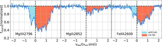
Average absorption profile for our sample of nine galaxy–absorber pairs. The Mg ii stack was obtained by calculating the mean of the profiles shown in the lower panel of Fig. 7. The stacks for Mg i and Fe ii were obtained in an identical way. As in Fig. 7, for those pairs where the galaxy rotation was blueshifted towards the quasar sightline, we flipped both galaxy and absorber velocities. Consequently, all co-rotation has positive velocities in these stacks (salmon), while all counter-rotating gas has negative velocities (light-blue).
6.2 Thin disc with pure circular orbits
In the previous section, we have tested, in a relatively general way, whether the gas probed by the low-α sightlines approximately shares the orientation of the angular momentum vector with the host galaxy. Drawing more quantitative conclusions from the LOS velocities is difficult, for two main reasons. First, an LOS velocity measurement does not allow one to get the 3D velocity vector of the probed gas. Secondly, the LOS probes gas at different spatial positions with different velocities. Therefore, quantitative conclusions can only be drawn using a parametrized model for the 3D density and kinematic of the gas.
The simplest possible model is to assume a thin disc which is spatially perfectly co-aligned with the galaxy disc, meaning that it can be understood as an extension of the galaxy disc. As the galaxy’s disc orientation in space – except for an ambiguity in the sign of the inclination – was determined by means of galpak3D modelling, we can predict where the sightline would cross such a (thin) disc.
Equation (8) shows that the LOS velocity vlos will always be smaller than the tangential velocity vϕ, i.e. vlos ≤ vϕ. However, the range of values for the ratio vlos/vϕ can be estimated for the range of allowed values in azimuthal angle α and inclination i imposed by our geometric selection (Section 4.3). For azimuthal angle ≲ 30°, which corresponds to the range in our sample, and inclinations in the range (40°–70°), equation (8) implies that vlos ranges from 0.5–0.9vϕ (|$=0.5{-}1.0\, v_\mathrm{\phi }\sin i)$|. Only for the highest inclinations (i > 70°), the range of values becomes very large, essentially from 0.0–1.0vϕ, with the sensitivity on the inclination depending on α. In other words, except for extreme inclinations, vlos is expected to be |$0.5{-}1.0\, v_\mathrm{\phi }\sin i$|.
While this range of values is consistent with our observations, this simple model would predict an absorption over a very narrow velocity range at vlos, whose width would be given by the disc turbulence (∼20–40 km s−1). In reality, we do not measure a single vlos, but the absorption profiles (or stacked profile) cover a relatively large range in velocities, from −0.5 to 1.5 vvirsin (i) (Fig. 8).
One possibility to explain the spread in the absorption profiles is to assume that the hypothesized disc has some thickness (e.g. Steidel et al. 2002; Kacprzak et al. 2010; Ho et al. 2017). In that case, the sightline intercepts the gaseous disc at different heights, corresponding to different radii R, leading to a range of projected vlos, even if the gas would be on pure circular orbits with a constant vϕ. However, this broadening effect would be a few tens of km s−1, and is not sufficient to explain the range of velocities in Fig. 8.
With the possible caveat of a very thick disc observed at high i, we assume that the peak velocity – the velocity where the optical depth reaches its maximum − as determined in Section 5.5, can be used as an estimator for vlos at the mid-plane. This LOS velocity vlos measured at ϕ and R can then be used to estimate the tangential velocity vϕ using equation (8).
Note that for sightlines with large azimuthal angle α (i.e. close to our selection limit of 40°) and for galaxies with very high inclination (i > 70°), the galactocentric radius can be very large and very uncertain. This affects especially J1107 and J1509.
This deprojected tangential velocity vϕ can then be compared to the circular velocity vcirc, taken to be ≈vvir, in order to assess whether the gas motion is consistent with stable circular orbits. Fig. 9 shows the ratio vϕ/vvir as a function of the galactocentric radius R (normalized by rvir). The error bars are large for J1107 and J1509, as expected from the discussion above. Excluding these two objects, there seems to be a trend with galacto-centric radius, in a sense that galaxies at smaller R/rvir are closer to being on stable circular orbits in the extended galaxy disc.

Tangential velocity vϕ inferred from vlos under the assumption that the gas is on pure circular orbits in the disc plane. For gas on stable circular orbits the expectation is that vϕ ≈ vvir. The two cases at the extreme ends of the vϕ/vvir distribution (J1107 cyan; J1509 purple, indicated by an arrow as outside of plot range) have both the highest α’s and inclinations among our nine galaxy–absorber pairs. The values of the plotted points are listed in Table C4 of the Supplementary Appendix.
This trend is also visible by simply looking at the absorption profiles in Fig. 7. We indicate in the lower panel of this figure the expected vlos for circular orbits with vvir at disc-mid-plane crossing. While in most of the cases the peak absorption is not coincident with the expected velocity, there is in many cases at least some absorption at the position of the exact co-rotation.
6.3 Disc with angular and radial motion – cold accretion discs
While the comparison between galaxy and halo gas absorption velocities for our sample strongly (Section 6.1) indicates that the halo gas probed by the low-ionization lines shares at least approximately the direction of the galaxy’s angular momentum vector, the previous section showed that the data are in most cases not consistent with the hypothesis that the gas is on stable circular orbits in a perfect extension of the galaxy discs.
Unfortunately, removing the constraint of perfect circular orbits and adding the possibility of inflow means that it is no longer possible to infer the velocity vector of the gas from the measured vlos, as there are in this scenario two unknowns for one measurement.
However, as discussed in Section 6.2 for the case of pure circular rotation, we can estimate the range of values for the tangential and radial terms in equation (10) imposed by our geometrical selection (Section 4.3). For the tangential term, the conclusion is similar as in Section 6.2, i.e. the numerical value ranges from |$0.5\,{\rm to}\,0.9\, v_\mathrm{\phi }$| for azimuthal angles α ≲ 30° and inclinations from 40° to 70°. For the radial term, the absolute value of the numerical factor ranges for this α and i range from 0.0 to 0.8. Unless the radial velocity |vr| is larger than the tangential component |vϕ|, the tangential component will typically dominate the LOS velocity vlos, regardless of geometrical factors, except when both i and α are large.
In order to break the degeneracy between radial and circular velocity, it is necessary to impose some additional information to reduce the dimensionality. Motivated by results from simulations one justifiable assumption is a constant vr (e.g. Rosdahl & Blaizot 2012; Goerdt & Ceverino 2015). By measuring vr directly from different simulations with different codes as a function of radius, redshift, and halo mass, Goerdt & Ceverino (2015) find that typical inflow velocities are approximately constant with radius at |$v_\mathrm{\mathit{ r}}\approx -0.6\, v_\mathrm{vir}$| for redshift z ≈ 1.
We now test the impact of the assumption of |$v_\mathrm{\mathit{ r}}=-0.6\, v_\mathrm{vir}$| and the possible signatures that this would have on our data. Such a radial component means that the magnitude of the radial term in equation (10) is thus at most |$|v_\mathrm{\mathit{ r}}|\lt 0.6\, v_\mathrm{vir}$|, while the tangential component is |${\approx } 0.5{-}0.9\, v_\mathrm{vir}$|, for inclinations less than 70° and α < 30°. This implies that discs with such a radial flow allow a wide range of LOS velocities vlos, from ≈0 to 1.1vvir in most general situations, i.e. except for the most extreme inclinations i > 70°, and thus can better reproduce the range of velocities observed in Fig. 8.
In Fig. 10, we use equation (11) to put constraints on vϕ for the galaxies in our sample with our assumption of vr = −0.6vvir. The resulting solutions for vϕ normalized by vvir are shown as a function of R/rvir. Solutions where the vlos contribution from vr shares the sign with the contribution from vϕ, are indicated as crosses, while solutions where they have the opposite sign are shown as diamonds. A case where the measured value does not give a co-rotating solution, but a co-rotating solution is possible within the uncertainties, is indicated by the small pink diamond at 0.36 for J2152.

Rotation velocities, vϕ, inferred from measured vlos under the assumption of a radial velocity component with vr = −0.6vvir and co-rotation with the galaxy for each of the nine absorbers. There can be up to two solutions per absorber. The projected LOS components of vr and vϕ have the same sign for solutions indicated by crosses, while they have opposite signs for solutions indicated by diamonds. The lines indicate different spin parameters (λ, see equation 12), with their values indicated in the legend. The values of the plotted points are listed in Table C4 of the Supplementary Appendix.
A first important conclusion from Fig. 10 is that, under the assumption of this infall velocity, there is for each absorber at least one solution consistent with 0 < vϕ/vvir < 1 in the co-rotating direction, even for the two cases which would in the absence of infall be interpreted to have a counter-rotating circular velocity.
6.4 Consequences for the angular momentum
Pure N-body simulations have shown that λ of the dark matter component integrated over the halo is approximately distributed with a lognormal distribution with |λ| = 0.035 and σ = 0.5, almost independent from redshift and halo mass (e.g. Bullock et al. 2001; Bett et al. 2007). Some hydrodynamical simulations predict that the cold accreting gas should have a higher λ on its way to the galaxy than the dark matter (e.g. Stewart et al. 2011b; Danovich et al. 2015; Teklu et al. 2015). For e.g. Danovich et al. (2015), using a similar simulation as Goerdt & Ceverino (2015), predict that the spin parameter λ for the cold gas, which we presumably probe with our data, scales with (R/rvir)0.5, and has approximately a λ = 0.06 at R/rvir = 0.1 and λ = 0.2 at R/rvir = 1.0.
We indicate in Fig. 10 the curves of constant λ = 0.03 (blue dotted line) and λ = 0.2 (orange dashed line). In addition, we show the curve λ = 0.2(R/rvir)0.5 (green solid line). All galaxy–absorber pairs except J2152 have within the uncertainties at least one solution within 0.03 < λ < 0.2. For most of the absorber pairs a solution with λ = 0.2(R/rvir)0.5 seems plausible, but also a solution with constant λ ≈ 0.03 is consistent with several of the absorbers.
6.5 Amount of accretion compared to star formation
Galaxies need to accrete gas from their halo. A plausible reservoir might be the extended cold gas discs probed by our sample. In Section 6.3, we have shown that the vlos measured for this gas are indeed consistent with infall rates and angular momenta predicted by simulations. Motivated by this, we can estimate the mass accretion rates from the Mg ii equivalent widths and the assumed infall velocities (vr = −0.6vvir).
Here the assumption is made that the disc is thin enough so that the column density perpendicular to disc can be estimated from the column density along the inclined view through |$\cos (i)\, N_\mathrm{H\,\small{I}}$|. Further, mp is the proton mass, and μ is the mean molecular weight, assumed to be 1.6. A further assumption is that all vϕ, vr, and the perpendicular column density do at fixed galacto-centric radius not depend on the disc azimuthal angle. The resulting |$\dot{M}_\mathrm{in}$| are listed in Table 8.

In Fig. 11, we compare the estimated |$\dot{M}_\mathrm{in}$| to the SFRs computed using the [O ii] luminosities with the extinction estimated from the M⋆–extinction relation of Garn & Best (2010) as described in Section 5.3. The dashed line shows the 1:1 relation, and the dotted lines are deviations from the 1:1 relation by a factor five. This figure shows that the estimated amount of |$\dot{M}_\mathrm{in}$| seems sufficient to balance the SFRs. Given that our estimate from equation (14) only takes account for the neutral component, the total |$\dot{M}_\mathrm{in}$| could be sufficiently higher if an ionized or molecular component would contribute to the inflow.
![Mass inflow rate estimated from ${{\rm Mg}\, \rm \small {II}}$ equivalent width plotted against SFR estimate obtained from [O ii] flux corrected for reddening using the E(B − V) estimate based on the Garn & Best (2010) M*–extinction relation. The dashed line represents an 1:1 relation. The dotted lines represent deviations from the 1:1 correspondence by a factor five.](https://oup.silverchair-cdn.com/oup/backfile/Content_public/Journal/mnras/485/2/10.1093_mnras_stz392/1/m_stz392fig11.jpeg?Expires=1750342074&Signature=jue6rGZi1Xv-cps8m~FH-VFriuNp~7OWA17G2mloDqQ-iwz6VB0wnm8iXsQAfdpt5vUEOdrfvg4L2wCcQJX7p2zFap2cLR6CNk5mcoTPD4PEUWN-fNy3vh1jw317mLQh9FKVPSB4zICajxNbzngN49qqcC08Xt1iNdaCt9PTO2qKE4K17ff3rpvgi1m7m5sr3H2SYyctdgPDwamTvHJJxv6g5UhfueTQqCvnpoc~Y1um77e3GgTMUpSGvjTWc-WEAMKM-5bDYNjH0OvzGV0DK3Bdc~dYY5XYrXhMS21bBBTbNNJQoTS6jaPY1Sm5ZEF8SWufgyDT1qnF78OBMR8ujA__&Key-Pair-Id=APKAIE5G5CRDK6RD3PGA)
Mass inflow rate estimated from |${{\rm Mg}\, \rm \small {II}}$| equivalent width plotted against SFR estimate obtained from [O ii] flux corrected for reddening using the E(B − V) estimate based on the Garn & Best (2010) M*–extinction relation. The dashed line represents an 1:1 relation. The dotted lines represent deviations from the 1:1 correspondence by a factor five.
7 SUMMARY AND CONCLUSIONS
Using our ongoing MEGAFLOW survey (Schroetter et al. 2016, Bouché et al. in preparation; Schroetter et al. in preparation), which targets galaxies around 79 strong Mg ii absorbers (with |${\mathrm{ EW}_0^{\lambda 2796}}\gtrsim 0.3{\mathring{\rm A} }$|) at z ≈ 1 with the VLT/MUSE spectrograph, we have investigated the distribution and kinematic properties of this low-ionization gas. Remarkably, the distribution of the azimuthal angle α for the galaxy–absorbers pairs within |$100\, {\rm kpc}$| shows a clear bi-modality (Fig. 2, top panel), which is highly suggestive of a CGM geometry with biconical outflows and extended gas discs. Our result confirms previous ones by Bouché et al. (2012), Kacprzak et al. (2012), and Bordoloi et al. (2011).
In light of this bimodal distribution, we have selected for this study the nine galaxy–absorber pairs which have the right orientation for the purpose of studying extended gaseous discs at galactocentric distances of 20–100kpc. This is the first statistical sample with both galaxy and absorber kinematics at z ≈ 1 specifically selected to study the cold gas discs.
Through a comparison of absorber and galaxy kinematics, we derived the following main conclusions:
There is little gas with vlos > vvirsin (i), which suggests that the gas in the disc is gravitationally bound to the halo (Section 6.1; Figs 7 and 8).
For seven out of the nine pairs the absorption velocity shares the velocity sign with the extrapolation of the galaxy rotation curve to the position of the quasar. This is the case for all four absorbers at b/rvir < 0.2 (Section 6.1; Fig. 7).
The inferred rotation velocity using the peak absorption velocity is in many cases smaller than vvir. This indicates that the gas is not on purely circular orbits. There seems to be a tendency for the discrepancy to be larger at larger impact parameters, with two cases at b/rvir > 0.25 even having counter-rotating velocities (Section 6.2; Fig. 9).
We investigated a scenario where the disc gas has a radial inflow (accretion component) in addition to the circular component, as predicted by simulations and required by indirect evidence. We showed that the data are consistent with inflow rates (vr ≈ −0.6vvir) and angular momentum distributions (Sections 6.3 and 6.4; Fig. 10) from simulations.
The inferred accretion rates are consistent with the expectation from the gas regulator (Bouché et al. 2010; Davé, Finlator & Oppenheimer 2012; Lilly et al. 2013) (Section 6.5; Fig. 11) and from hydrodynamical calculations (e.g. Faucher-Giguère et al. 2011; Nelson et al. 2015; Correa et al. 2018).
For some of the conclusions listed above we needed to make relatively strong assumptions. For example, we assumed that the gas is in a perfect extension of the galaxy disc and the angular momentum vector of the gas is perfectly aligned with the galaxy. This is not exactly what simulations predict for the cold streams falling into the halo, and only to some extent the case for the cold-accretion discs into which the streams supposedly settle in the inner halo. In addition, extended gas discs might be warped. While the gas needs to finally align with the galaxy disc, how this alignment happens and out to where it persists is far from a solved question. In simulations it seems to depend on the code and the feedback implementations (e.g. Stewart et al. 2017). However, reassuringly our α histogram shows that the gas that we probe with Mg ii needs to be at least in a discy structure.
The finding of gravitationally bound co-rotating gas is consistent with a range of quasar-absorption studies for individual objects with the right geometry ranging up to z ≈ 2 (e.g. Barcons et al. 1995; Steidel et al. 2002; Bouché et al. 2013, 2016; Bowen et al. 2016; Rahmani et al. 2018). The only other study that systematically selected a statistical sample with the right geometry for the purpose of studying extended cold gas discs was recently performed by Ho et al. (2017). Importantly, their work is targeting galaxies at significantly lower redshift, z ≈ 0.2, and hence can be considered complementary to our study. Qualitatively they find at this lower redshift a similar result as we do: The majority of the Mg ii absorption profiles matches the sign of the galaxy rotation (8 out of their 12 robust galaxy–absorber identifications). Similarly to us, they also find that the majority of the gas has vϕ < vcirc. Combining this with the fact that for some systems part of the absorption counter-rotates, they also conclude – for z ≈ 0.2 – that the gas likely has a radial infall component.
SUPPORTING INFORMATION
Appendix A. Uncertainties of inclination and azimuthal angle estimates.
Appendix B. Field, spectral, and kinematic plots for each of the absorbers.
Appendix C. Supplementary tables.
Appendix D. Supplementary figures.
Please note: Oxford University Press is not responsible for the content or functionality of any supporting materials supplied by the authors. Any queries (other than missing material) should be directed to the corresponding author for the article.
ACKNOWLEDGEMENTS
We thank the anonymous referee for a careful and constructive report, which helped to improve the quality of the manuscript. This work has been carried out thanks to the support of the Agence Nationale de la Recherche (ANR) grant FOGHAR (ANR-13-BS05-0010), the ANR grant 3DGasFlows (ANR-17-CE31-0017), the OCEVU Labex (ANR-11-LABX-0060), and the A*MIDEX project (ANR-11-IDEX-0001-02) funded by the ‘Investissements d’avenir’ French government program. LW acknowledges support by the Competitive Fund of the Leibniz Association through grant SAW-2015-AIP-2.
This work made use of the following open source software: galpak3D (Bouché et al. 2015), zap (Soto et al. 2016b), mpdaf (Piqueras et al. 2017), matplotlib (Hunter 2007), numpy (Oliphant 2007; van der Walt, Colbert & Varoquaux 2011), astropy (Astropy Collaboration et al. 2013), montage (Jacob et al. 2010). This study is based on observations collected at the European Southern Observatory under ESO programmes 094.A-0211(B), 095.A-0365(A), 096.A-0609(A), 096.A-0164(A), 097.A-0138(A), 097.A-0144(A), 098.A-0216(A), 098.A-0310(A), 099.A-0059(A), 293.A-5038(A).
Footnotes
[O ii] can be observed with MUSE starting from z ≈ 0.3, but the JHU-SDSS Mg ii catalogue does not include absorbers below z = 0.4.
This was the period of data used for our first full analysis of the data, which is the basis for this paper and a companion paper discussing outflows (Schroetter et al. in preparation). Observations were completed in 2018 November.
Starting with version v2.4 of the muse drs, which was not available at the time when we reduced the data for this work, the self-calibration is directly implemented. The steps described in this paragraph would no longer be necessary when using drs v2.4 or later.
A ‘pixtable_positioned’ is a pixtable where the spatial position information for each pixel is given in absolute RA and Dec.
The width of the [O ii] NB filters was extended by the width of the separation of the [O ii] doublet.
This galaxy shows clear AGN signatures, e.g. a strong |${[{\rm Ne}\, \rm \small {V}}]{}\, \lambda \lambda 3346,3426$| detection (Mignoli et al. 2013). While this doublet is not detected in any of the nine remaining galaxies, we cannot rule out AGN contribution with certainty for the sample based on the available data.
Available at https://bitbucket.org/bepinat/camel.git.
We use a fixed line ratio of 0.8:1.0 per default, except when the observed [O ii] doublet ratio deviates strongly from 0.8.
We converted the Amorisco & Bertin (2010) relation between the exponential disc scale length and the radius where the rotation curve reaches 2/3 of vmax to a rhalf and rturn ratio for an arctan rotation curve.
Alternatively, one could correct the z = 0 Kewley et al. (2004) |$L_{{[{\rm O}\, \rm \small {II}}];\rm i}\text{--}E(B-V)$| relation by taking into account the MS redshift evolution (SFR∝(1 + z)α; with α ≈ 2–3).
The product vmaxsin (i) ≈ vvirsin (i) can be accurately measured even if the inclination itself cannot be well constrained.
