-
PDF
- Split View
-
Views
-
Cite
Cite
N Wang, Q Y Peng, X Zhou, X Y Peng, H W Peng, A distortion solution for the Bok telescope with four CCD chips, Monthly Notices of the Royal Astronomical Society, Volume 485, Issue 2, May 2019, Pages 1626–1634, https://doi.org/10.1093/mnras/stz459
Close - Share Icon Share
ABSTRACT
The Beijing–Arizona Sky Survey (BASS) is an imaging survey that uses the 2.3-m Bok telescope at Kitt Peak. In order to realize the astrometric potential of the Bok telescope and improve the astrometry of BASS, a distortion solution for the Bok telescope is needed. In the past, we used a single lookup table to correct all the positional errors. However, this method cannot be applied to the reduction of observations from the Bok telescope, which is equipped with four CCD chips. We thus developed a method that is quite different from our previous one, using two third-order polynomials to fit the lookup table. By using the polynomial geometric distortion (GD) correction, the astrometry of BASS is greatly improved. Moreover, an additional lookup-table correction is found to be more effective to obtain the final GD. The results show that the positional measurement precision of the appropriate bright stars is estimated at about 20 mas or even better in each direction. In addition, the relative positions of the chips are measured. The change of the inter-chip gaps in the horizontal or vertical is no more than 5 pixels between 2016 and 2017, and the change of the roll angle is no more than 0|${^{\circ}_{.}}$|1.
1 INTRODUCTION
The Beijing–Arizona Sky Survey (BASS) is a new g- and r-band imaging survey conducted by the National Astronomical Observatory of China (NAOC) and the Steward Observatory (Zou et al. 2017). BASS uses the 2.3-m Bok telescope, which is located at Kitt Peak has a 90Prime camera installed at the prime focus. The camera is composed of four 4096 × 4032 CCDs and provides a field of view of about 1 deg2. The depths of the single-epoch images are about 23.4 m and 22.9 mag for g and r, respectively. The typical exposure time is about 60 s, depending on the meteorological conditions. BASS, the Dark Energy Camera Legacy Survey (Blum et al. 2016) and the MOSAIC z-band Legacy Survey (Silva et al. 2016) constitute the Dark Energy Spectroscopic Instrument (DESI) imaging surveys. BASS will survey about 5400 deg2 in the northern Galactic cap and provide spectroscopic targets for DESI. In addition, BASS will provide unique scientific opportunities for studying Galactic halo substructures, satellite dwarf galaxies around the Milky Way, galaxy clusters, high-redshift quasars, and so on (Zou et al. 2017). Table 1 summarizes the specifications of the Bok telescope and the CCD detector.
| Telescope . | 2.3-m Bok . |
|---|---|
| F-ratio | f/2.98 |
| Diameter of primary mirror | 230cm |
| Absolute pointing | <3arcsec rms |
| CCD field of view | 1.08° × 1.03° |
| Size of CCD array | 4096 × 4032 |
| Size of pixel | 15μm × 15μm |
| Approximate angular extent per pixel | 0.454 arcsec pixel-1 |
| Typical exposure time | 60 s |
However, the astrometry of BASS is unsatisfactory. The astrometric solutions of BASS are derived by cross-identifying objects in the frames with the SDSS and 2MASS star catalogues (Zhou et al. 2016). During the first data release of BASS, the median positional errors of stars from 9000 frames in right ascension and declination were about 0.10 and 0.11 arcsec, respectively (Zou et al. 2017). There are several factors that affect the accuracy of astrometric solutions, such as the precision of the source positional measurements, the solution of the geometric distortion (GD), the positional precision of the reference stars, and so on. Among these factors, the solution of the GD is particularly important. In general, there are two ways to derive the GD. The direct way is to observe an astrometric flat-field in which we have prior knowledge of the positions of all the stars in some absolute and accurate system (Anderson & King 2003). The distortion is then obtained by means of the residuals. However, such a standard calibration field is usually not available owing to the lack of precision and star density. Although Gaia Data Release 1 (DR1) (Gaia Collaboration et al. 2016b,a) can provide positional precision and star density, the lack of proper motion for most of the stars can induce non-negligible errors. It is, however, expected that the release of Gaia DR2 (Gaia Collaboration et al. 2018) will lead to good results. The other way is to take advantage of the instrument itself to calibrate. Anderson et al. (2006) applied the self-calibration method to wide-field ground-based images and achieved good precision. Peng et al. (2012) presented an alternative self-calibration method and successfully applied the method to the observations of some natural satellites (Peng et al. 2015; Wang et al. 2017; Peng, Peng & Wang 2017). The self-calibration method is therefore more practical and effective than the former method, because the derivation of the GD is free from the errors of the star catalogue in position and proper motion; however, additional observations of the calibration field should be made. According to Peng et al. (2012), observations of the calibration field should be made at different offsets in a dithered pattern of either ‘+’ or ‘|$\#$|’. The offset between any two neighbouring exposures should be appropriate, and the size of the offset depends on the change of the GD pattern. The field of view of the Bok telescope is quite wide, and thus much requirement for the offset should be met (such as more reference stars, smaller offsets and so on). However, during the exposures of the same sky field for BASS, the offset between two neighbouring exposures is about 10 arcmin in right ascension or declination, see Fig. 1. Owing to the insufficient overlap area, the derived lookup table is inadequate, and the positional precision of the stars is affected. Thus two third-order polynomials were tried beyond the numerical GD model. The results show that the positional precision of the stars is much improved after the third-order polynomial GD correction. Here, the averaged GD in a small box (see Section 3.1) is referred to as the numerical GD, and the GD derived from a polynomial is referred to as the analytical GD. Moreover, a precise pixel positional measurement is fundamental. During the pixel positional measurement, a two-dimensional Gaussian fit was used to obtain the precise positions of the stars (Li, Peng & Han 2009), as was done in our previous works (Peng et al. 2015; Wang et al. 2015, 2017). In addition, in order to correct all the smaller-scale systematic positional errors, an additional lookup table correction was found to be useful.

Dithered observational scheme for the CCD frames in 2016. The 49 images are organized in a 7 × 7 array. The units are degrees. The observational scheme for 2017 is similar to that for 2016.
This paper is organized as follows. Section 2 describes the observations. Section 3 presents the solution of the GD models. Section 4 analyses the relative positions of the chips. Finally, Section 5 draws some conclusions.
2 OBSERVATIONS WITH DIFFERENT FILTERS
Before each night of observations, the x-axis of each CCD chip was set to be nearly parallel to the real equator by a star-trailing operation. Two sets of observations were taken, in 2016 and 2017 (see Table 2). All the observations were made with the 2.3-m Bok telescope at Kitt Peak. The site (IAU code 691) is at longitude E248° 24′ 3|${^{\prime\prime}_{.}}$|6, latitude N31° 57′ 28|${^{\prime\prime}_{.}}$|7 and height 2079.8 m above sea level. The exposure time for each CCD frame was 60 s, and the pixel scale was about 0|${^{\prime\prime}_{.}}$|454. The observations in 2016 were made at high galactic latitude, and in each frame a small number of reference stars (∼300 stars) were available. The centre of the field of observation was at E162|${^{\circ}_{.}}$|05 in right ascension, N28|${^{\circ}_{.}}$|65 in declination. The observations in 2017 were made at low galactic latitude, and plenty of reference stars (∼3200 stars) were available in each frame. The centre of the field was at E147|${^{\circ}_{.}}$|35 in right ascension, N1° in declination. An exposure included four frames, and a total of 4 × 87 frames of CCD images were obtained in a dithered pattern (see Fig. 1). There was an inter-chip gap at the centre of the array, see Fig. 2 (Zou et al. 2017). The Bok telescope has an equatorial mount, and other information about the telescope and the observations can be found from the FITS header. A sample FITS header is provided in the Appendix.
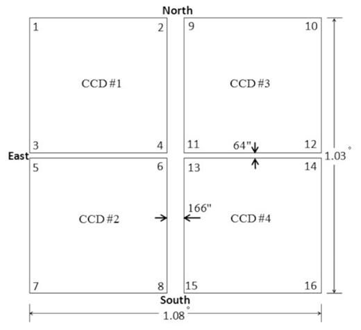
Layout of the CCD array. There are four CCDs: CCD|$\#$|1, CCD|$\#$|2, CCD|$\#$|3, CCD|$\#$|4, and four identifiers are listed at the corners of each CCD. An exposure includes four CCD frames. (See fig. 1 in Zou et al. 2017.)
Observations for the calibration field. Column 2 lists the number of CCD frames and column 3 lists the filter.
| Observation date . | No. of calibration fields . | Filter . |
|---|---|---|
| 2016-01-17 | 4 × 49 | r |
| 2017-03-05 | 4 × 38 | g |
| Observation date . | No. of calibration fields . | Filter . |
|---|---|---|
| 2016-01-17 | 4 × 49 | r |
| 2017-03-05 | 4 × 38 | g |
3 SOLVE FOR THE GD MODELS SUCCESSIVELY
The reduction procedures were carried out according to Peng et al. (2012). First, a numerical GD model was derived. Then an analytical GD model was tried, because the residuals of the stars were still large after the numerical GD correction. After the analytical GD correction, the positional precision of stars was much improved. Finally, an additional lookup table was set up because the residual GD does not converge for the preset threshold. Further explanations are given below.
3.1 The derivation of the numerical GD model
The derivation of the numerical GD model involved the following main steps. (1) Information about the date of the observation, exposure time, and so on was extracted automatically from the FITS header by our own software (Peng et al. 2017; Wang et al. 2017). Then, after some pre-processing (de-bias, flat correction), the pixel positions of the stars in each CCD frame were measured with a two-dimensional Gaussian fit; this is different from the procedure used previously, when SExtractor (Bertin & Arnouts 1996) was used for the pixel positional measurements. Because the solution of the GD can be affected by the precision of bright stars (brighter than 14 mag and saturated), these stars were not considered. For each CCD frame in 2016, about 100 stars were rejected and about 200 stars were used. For each CCD frame in 2017, about 200 stars were rejected and about 3000 stars were used. The stars in each frame were then matched with the stars in the Gaia DR2 star catalogue using a fast matching algorithm (Ren & Peng 2017). The pixel positional measurement and the match process were performed automatically by our own software. (2) For each chip, we adopted the centre of the CCD array as the tangential point on the tangential plane of the image. The standard coordinates of the stars were then obtained by the central projection (Green 1985). Next, the positional residuals (observed minus averaged; O − A) of the stars were obtained after four-parameter transformation. Because an accurate GD model requires a high precision for the positions of the stars, the topocentric apparent position and atmospheric refraction for each matched star in each CCD frame were also taken into account during the computations of the standard coordinates. (3) Owing to the high number of reference stars available in 2017, each CCD frame was divided into 1024 equal-area boxes, with the size of each box equal to 128 × 126 pixels. Each CCD frame in 2016 was divided into 256 boxes, with the size of each box equal to 256 × 252 pixels. The averaged GD in each box was then obtained by cancelling out the catalogue errors and compressing the measured errors. After 10 to 12 iterations, the numerical GD converged and was derived. In fact, the derived numerical GD model is a lookup table.
Figs 3 and 4 show the numerical GD patterns for the Bok telescope in 2016 and 2017, respectively. It can be seen that the telescope suffers from a serious GD, especially in the corners. The maximum GD is about 22 pixels (∼10.18 arcsec). Figs 5 and 6 show the positional residuals of the stars with respect to the magnitude in 2016 and 2017, respectively. It can be seen that the positional residuals are suppressed largely after the numerical GD correction.

Geometric distortion (GD) for the Bok 2.3-m telescope. The GD was derived from the observations in 2016 and the r-filter was used. The maximum GD (Max) and the median GD (Med) are listed in units of pixels, and a factor of 20 is used to exaggerate the magnitude of the GD vectors.
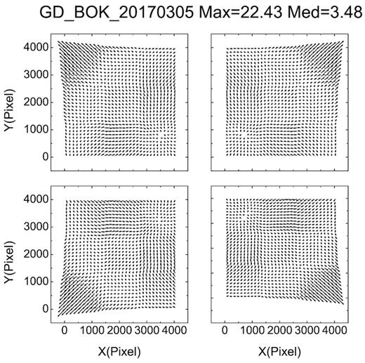
Geometric distortion (GD) for the Bok 2.3-m telescope. The GD was derived from the observations in 2017 and the g-filter was used. The maximum GD (Max) and the median GD (Med) are listed in units of pixels, and a factor of 20 is used to exaggerate the magnitude of the GD vectors.
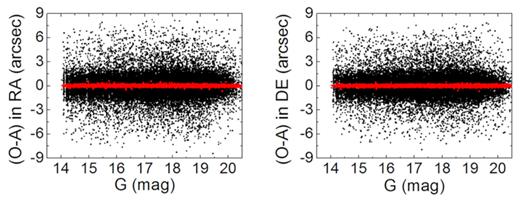
Observed minus averaged (O − A) residuals of the stars in 2016. The dark points represent the residuals before the numerical GD correction, where four-parameter transformation is used, and the red ones represent the residuals after the numerical GD correction.
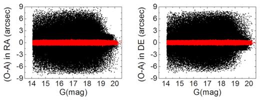
Observed minus averaged (O − A) residuals of the stars in 2017. The dark points represent the residuals before the numerical GD correction, where four-parameter transformation is used, and the red ones represent the residuals after the numerical GD correction.
3.2 Derivation of the analytical GD model
By using the numerical GD correction, the precision of the stars is improved. However, the positional residuals of the stars are still large. Specifically, we found that the residuals were not distributed randomly with respect to the stars’ pixel positions (see Figs 7 and 8). Furthermore, the GD pattern in 2017 seems to be divided into several blocks (see Fig. 4). The analytical GD model was thus tried after the numerical GD model.
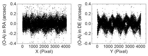
Positional residuals of the stars with respect to the pixel positions in 2016.

Positional residuals of the stars with respect to the pixel positions in 2017.
After fitting, the coefficients of the polynomial were obtained and the analytical GD model was derived. Next an iterative procedure is necessary.
Table 3 lists the solved coefficients of the third-order polynomials in 2016 and 2017, respectively, and Figs 9 and 10 show the positional residuals of the stars with respect to the magnitude. From Figs 9 and 10 it can be seen that the positional precision of the stars is much improved. The final GD correction reaches a positional precision level of ∼0.05 pixel (∼22 mas) in each coordinate, and most of the GD is removed. The definition of the precision of the GD correction can then be given; that is, the precision of the GD correction can be denoted by the star positional residual after the GD correction.

Positional residuals of the stars with respect to the magnitude in 2016. The black points represent the residuals after the numerical GD correction, and the red ones represent those after the analytical GD correction.
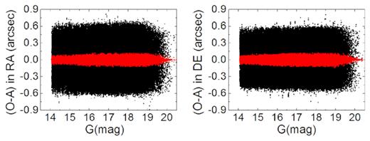
Positional residuals of the stars with respect to the magnitude in 2017. The black points represent the residuals after the numerical GD correction, and the red ones represent those after the analytical GD correction.
The coefficients of the analytical model for the observations in 2016 and 2017. Column 1 lists the designation of each CCD chip, and column 2 lists the date. Column 3 lists the direction (|${a}$| or |${b}$|). Columns 4 to 13 list the coefficients of the polynomials.
| CCD . | Date . | . | 1 . | 2 . | 3 . | 4 . | 5 . | 6 . | 7 . | 8 . | 9 . | 10 . |
|---|---|---|---|---|---|---|---|---|---|---|---|---|
| |$\#$|1 | 2016 | a | 1.897 | 0.090 | 1.857 | 0.020 | −6.256 | −3.953 | −2.039 | −0.658 | 2.335 | 2.754 |
| 2016 | b | 0.024 | 1.875 | 0.068 | 2.065 | −1.962 | −4.186 | −5.744 | 6.392 | −1.371 | 2.559 | |
| |$\#$|2 | 2016 | a | 1.880 | −0.068 | 1.856 | −0.021 | −6.264 | 3.694 | −2.041 | 0.038 | −2.298 | 2.757 |
| 2016 | b | −0.068 | 1.848 | −0.057 | 1.909 | 1.820 | −4.195 | 5.373 | −5.936 | −1.052 | −2.388 | |
| |$\#$|3 | 2016 | a | 1.889 | −0.090 | 1.855 | −0.037 | 5.871 | −3.973 | 1.913 | −1.820 | −1.426 | −2.585 |
| 2016 | b | −0.027 | 1.874 | −0.085 | 1.904 | −1.978 | 3.896 | −5.799 | −6.813 | −1.791 | 2.582 | |
| |$\#$|4 | 2016 | a | 1.886 | 0.087 | 1.865 | 0.035 | 5.906 | 3.687 | 1.937 | −0.153 | 2.474 | −2.604 |
| 2016 | b | 0.036 | 1.878 | 0.082 | 1.910 | 1.831 | 3.932 | 5.354 | 5.114 | −0.825 | −2.385 | |
| |$\#$|1 | 2017 | a | 1.942 | 0.084 | 1.857 | 0.015 | −6.333 | −4.049 | −2.044 | −1.198 | 4.493 | 2.790 |
| 2017 | b | 0.023 | 1.885 | 0.074 | 1.889 | −2.020 | −4.200 | −5.877 | 4.389 | −1.613 | 2.630 | |
| |$\#$|2 | 2017 | a | 1.926 | −0.030 | 1.867 | −0.005 | −6.308 | 3.668 | −2.025 | −0.383 | −4.012 | 2.775 |
| 2017 | b | −0.002 | 1.881 | −0.027 | 1.873 | 1.813 | −4.150 | 5.364 | −4.091 | −1.589 | −2.390 | |
| |$\#$|3 | 2017 | a | 1.922 | −0.032 | 1.829 | −0.019 | 5.987 | −4.069 | 1.929 | −1.559 | −4.398 | −2.636 |
| 2017 | b | −0.009 | 1.861 | −0.031 | 1.830 | −2.051 | 3.919 | −5.922 | −4.093 | −1.329 | 2.655 | |
| |$\#$|4 | 2017 | a | 1.911 | 0.052 | 1.878 | 0.007 | 6.010 | 3.643 | 1.941 | −0.852 | 3.845 | −2.648 |
| 2017 | b | 0.013 | 1.898 | 0.049 | 1.832 | 1.810 | 3.913 | 5.316 | 3.663 | −1.612 | −2.373 |
3.3 Setting up an additional lookup table
Although the precision for a star’s reduced position is greatly improved after the analytical GD correction, during the iterative solution of the analytical GD model, the numerical GD does not converge for the preset threshold, for example 0.01 pixel. Therefore an additional lookup table was set up, and the corresponding lookup-table correction was followed after the analytical GD correction. After the lookup-table correction, the numerical GD converged quickly during the iterative solution. Figs 11 and 12 show the analytical GD patterns for the Bok telescope in 2016 and 2017, respectively. From Fig. 12 it can be seen that the blocks found in Fig. 4 have disappeared. In order to show the result of the GD correction, the final residual patterns after the analytical GD correction and the lookup-table correction are also shown in Figs 13 and 14, where the magnitude of the residual is magnified by a factor of 20 000.

Geometric distortion (GD) for the Bok 2.3-m telescope in 2016. The GD was derived from the analytical GD model and the additional lookup table in 2016. The maximum GD (Max) and the median GD (Med) are listed in units of pixels, and a factor of 20 is used to exaggerate the magnitude of the GD vectors.

Geometric distortion (GD) for the Bok 2.3-m telescope in 2017. The GD was derived from the analytical GD model and the additional lookup table in 2017. The maximum GD (Max) and the median GD (Med) are listed in units of pixels, and a factor of 20 is used to exaggerate the magnitude of the GD vectors.
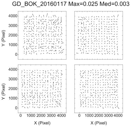
Residuals for the Bok 2.3-m telescope in 2016. The maximum geometric distortion (GD) (Max) and the median GD (Med) are listed in units of pixels, and a factor of 20 000 is used to exaggerate the magnitude of the GD vectors.

Residuals for the Bok 2.3-m telescope in 2017. The maximum geometric distortion (GD) (Max) and the median GD (Med) are listed in units of pixels, and a factor of 20 000 is used to exaggerate the magnitude of the GD vectors.
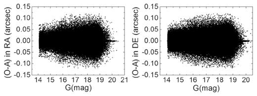
In addition, Figs 15 and 16 show the positional residuals of the stars after the analytical GD correction and the additional lookup-table correction. Table 4 shows the mean and standard deviation of the stars’ positional residuals using the different GD models. From Figs 15, 16 and Table 4 it can be seen that the positional precision of the stars is further improved. Furthermore, the positional residuals of the stars with respect to the pixel positions are shown in Figs 17 and 18. From these two figures, it can be seen that the positional residual is distributed almost randomly after the analytical GD correction and the additional lookup-table correction. However, a small hopping is seen in the right panel of Fig. 17, and further study of this pattern needs to be undertaken. Table 5 shows the mean and standard deviation of the stars’ positional residuals using different orders of polynomial fit. Fig. 19 shows the standard deviation of each star’s positional residual in 2016 in right ascension and declination, and Fig. 20 shows the standard deviation in 2017. In Figs 19 and 20, the stars that appear more than twice are included, and a smooth line is drawn for every 500 points. In short, from these figures we can see that after the GD correction, the positional measurement precision for the bright stars is better than 20 mas. The positional measurement precision in 2017 is even better for most stars.
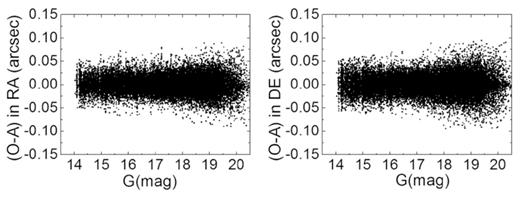
Positional residuals of the stars with respect to the magnitude in 2016 in right ascension (left) and declination (right). The black points represent the residuals of the stars after the analytical geometric distortion (GD) correction and the additional lookup-table correction.
Positional residuals of the stars with respect to the magnitude in 2017 in right ascension (left) and declination (right). The black points represent the residuals of the stars after the analytical geometric distortion (GD) correction and the additional lookup-table correction.
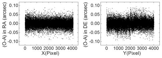
Positional residuals of the stars with respect to the pixel positions in 2016. The dark points represent the residuals after the analytical geometric distortion (GD) correction and the additional lookup-table correction.
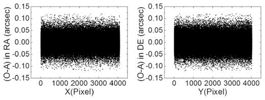
Positional residuals of the stars with respect to the pixel positions in 2017. The dark points represent the residuals after the analytical geometric distortion (GD) correction and the additional lookup-table correction.
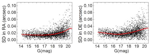
Standard deviation of the positional residual for each star after the analytical geometric distortion (GD) correction and the additional lookup-table correction with respect to the magnitude in 2016. A Savitzky–Golay smooth line is drawn for every 500 points.
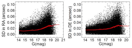
Standard deviation of the positional residual for each star after the analytical geometric distortion (GD) correction and the additional lookup-table correction with respect to the magnitude in 2017. A Savitzky–Golay smooth line is drawn for every 500 points.
Statistics of the positional residuals for all stars using different geometric distortion (GD) models for each data set. Column 1 is the date. Column 2 gives the GD model. The following columns list the mean positional residual and its standard deviation (SD) in right ascension and declination, respectively. All units are arcseconds.
| Date . | GD model . | <O − A> . | SD . | <O − A> . | SD . |
|---|---|---|---|---|---|
| . | . | RA . | Dec. . | ||
| 2016-01-17 | Analytical | 0.000 | 0.019 | 0.000 | 0.023 |
| Analytical+lookup table | 0.000 | 0.018 | 0.000 | 0.021 | |
| 2017-03-05 | Analytical | 0.000 | 0.019 | 0.000 | 0.021 |
| Analytical+lookup table | 0.000 | 0.018 | 0.000 | 0.020 | |
Statistics of the positional residuals for all stars after the analytical GD correction and the additional lookup-table correction using different orders of polynomial fit. Column 1 is the date. Column 2 lists the order of the polynomial fit. The following columns list the mean positional residual and its standard deviation (SD) in right ascension and declination, respectively. All units are arcseconds.
| Date . | Order . | <O − A> . | SD . | <O − A> . | SD . |
|---|---|---|---|---|---|
| . | . | RA . | Dec. . | ||
| 2016-01-17 | 2 | 0.000 | 0.035 | 0.000 | 0.039 |
| 3 | 0.000 | 0.018 | 0.000 | 0.021 | |
| 4 | 0.000 | 0.018 | 0.000 | 0.021 | |
| 5 | 0.000 | 0.018 | 0.000 | 0.021 | |
| 2017-03-05 | 2 | 0.000 | 0.047 | 0.000 | 0.049 |
| 3 | 0.000 | 0.018 | 0.000 | 0.020 | |
| 4 | 0.000 | 0.018 | 0.000 | 0.020 | |
| 5 | 0.000 | 0.018 | 0.000 | 0.020 | |
4 RELATIVE POSITIONS OF THE CHIPS
Owing to the accurate GD pattern, it is convenient to know the relative positions of the CCD array. Because the centre of the CCD array was adopted as the tangential point on the tangential plane, the standard coordinates for each pixel can be computed and the inter-chip gaps can be obtained. We use CCD|$\#$|2 and CCD|$\#$|3 as a reference to compute the inter-chip gap for each observational set (see Fig. 2). Because the inter-chip gaps were derived from the extrapolation of the final GD model, the far distance from the reference chip’s boundary was not reliable for the measurement of the inter-chip gaps. As such, only 12 points were given to compute their positional changes. When CCD|$\#$|2 is used as the reference, the pixel positions for the corners 5, 6 and 8 are (0.5, 4031.5), (4031.5, 4031.5) and (4031.5, −0.5). When CCD|$\#$|3 is used as the reference, the pixel positions for the corners 9, 11 and 12 are (0.5, 4031.5), (0.5, −0.5) and (4031.5, −0.5). The pixel positions for the other corners are listed in Table 6.
The positions of the points at the corners (see Fig. 2). Columns 2 to 9 show the mean pixel positions and their corresponding standard deviations. The top panel uses CCD|$\#$|2 as the reference, and the bottom one uses CCD|$\#$|3. All units are pixels.
| Corner . | 3 . | 4 . | 13 . | 15 . | ||||
|---|---|---|---|---|---|---|---|---|
| Date . | <mean> . | SD . | <mean> . | SD . | <mean> . | SD . | <mean> . | SD . |
| 2016 | (−7.029,4177.380) | (0.063,0.059) | (4024.407,4178.564) | (0.069,0.089) | (4472.624,4012.683) | (0.042,0.242) | (4464.065,−17.983) | (0.034,0.059) |
| 2017 | (−10.275,4173.382) | (0.049,0.095) | (4020.632,4175.989) | (0.059,0.092) | (4467.475,4009.499) | (0.033,0.052) | (4460.441,−21.430) | (0.038,0.056) |
| Corner | 2 | 4 | 13 | 14 | ||||
| Date | <mean> | SD | <mean> | SD | <mean> | SD | <mean> | SD |
| 2016 | (−363.701,4053.247) | (0.039,0.067) | (−366.320,22.462) | (0.032,0.193) | (24.878,−148.552) | (0.063,0.073) | (4056.526,−135.165) | (0.051,0.082) |
| 2017 | (−362.698,4052.952) | (0.040,0.048) | (−365.073,22.179) | (0.042,0.060) | (20.084,−141.796) | (0.066,0.100) | (4050.305,−133.761) | (0.063,0.102) |
Fig. 21 shows the change of the inter-chip gap when CCD|$\#$|2 is used as the reference in 2016 and 2017, respectively, and Fig. 22 shows the change of the inter-chip gap when CCD|$\#$|3 is used as the reference. From Figs 21 and 22 it can be seen that there was a slight shift in the inter-chip gap in 14 months. Furthermore, Fig. 23 shows the change of the inter-chip gap, and Fig. 24 shows the change of the roll angles between 2016 and 2017 with respect to CCD|$\#$|2 (chosen as the reference). The statistics of inter-chip gaps and the roll angles in 2016 and 2017 are shown in Table 7. From Table 7 it can be seen that the change of the roll angle in 14 months is no more than 0|${^{\circ}_{.}}$|1 and that the roll angles appear to be stable.

The change of the inter-chip gap when CCD|$\#$|2 is used as the reference. The left panel shows the change in the horizontal, and the right panel shows the change in the vertical. The black line shows the change in 2016, and the red line shows the change in 2017.
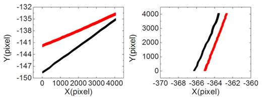
The change of the inter-chip gap when CCD|$\#$|3 is used as the reference. The left panel shows the change in horizontal, and the right panel shows the change in vertical. The black line shows the change in 2016, and the red line shows the change in 2017.

The change of the inter-chip gap in 2016 and 2017. The left panel shows the change of the vertical gap with respect to CCD|$\#$|2, and the right panel shows the change of the horizontal gap.

The change of the roll angle in 2016 and 2017. The left panel shows the change of chip|$\#$|1 with respect to CCD|$\#$|2, and the right panel shows the change of chip|$\#$|4 with respect to CCD|$\#$|2.
Statistics of the inter-chip gaps and the roll angles. ‘16gap’ is the abbreviation for the gap in 2016. ‘16angle’ is the abbreviation for the angle in 2016. Columns 2 to 9 show the averaged values and the standard deviation for the gaps and the angles. CCD|$\#$|2 and CCD|$\#$|3 are used as the reference. The unit for rows 1 and 2 is arcsec and for rows 3 and 4 is degrees. The unit of the standard deviation for rows 3 and 4 is arcmin.
| Date . | <mean> . | SD . | <mean> . | SD . | <mean> . | SD . | <mean> . | SD . |
|---|---|---|---|---|---|---|---|---|
| Parameter . | CCD1(CCD2) . | CCD4(CCD3) . | CCD4(CCD2) . | CCD1(CCD3) . | ||||
| 16gap | 66.13 | 0.03 | 64.20 | 0.03 | 168.58 | 0.01 | 165.09 | 0.02 |
| 17gap | 64.63 | 0.04 | 62.38 | 0.04 | 166.53 | 0.01 | 164.63 | 0.02 |
| 16angle | 0.013 | 0.06 | 0.190 | 0.02 | 89.879 | 0.12 | 89.961 | 0.06 |
| 17angle | 0.037 | 0.03 | 0.115 | 0.02 | 89.901 | 0.00 | 89.965 | 0.00 |
5 CONCLUSION
Although the Bok telescope provides favourable astrometric properties, the GD must be solved carefully. The distortion solution for BASS on the Bok telescope presented here is quite different from the previous method, where the numerical GD model was enough. Instead of the numerical GD model, an analytical GD model and additional lookup table were used to improve the astrometry of BASS. After the analytical GD correction and the additional lookup-table correction have been applied, the internal agreement or precision of the stars is estimated at about 20 mas or even better in each direction. This improvement means that the astrometric potential of the Bok telescope can be realized and the telescope can be used to carry out research into reference frames, brown dwarfs, parallax, proper motion, and so on.
ACKNOWLEDGEMENTS
We acknowledge the support of the staff of the National Astronomical Observatory of China and the staff of the Bok telescope at Steward Observatory. This work was supported by the Joint Research Fund in Astronomy (U1431227) under cooperative agreement between the National Natural Science Foundation of China (NSFC) and the Chinese Academy of Sciences (CAS), by the National Natural Science Foundation of China (Grant No. 11703008, 11873026), the Natural Science Foundation of Guangdong Province, China (Grant No. 2016A030313092), the Opening Project of Guangdong Province Key Laboratory of Computational Science at Sun Yat-sen University, and partly by the Fundamental Research Funds for the Central Universities. This work has made use of data from the European Space Agency (ESA) mission Gaia (https://www.cosmos.esa.int/gaia), processed by the GaiaData Processing and Analysis Consortium (DPAC, https://www.cosmos.esa.int/web/gaia/dpac/consortium). Funding for the DPAC has been provided by national institutions, in particular the institutions participating in the Gaia Multilateral Agreement.
REFERENCES
APPENDIX A: The header of the Bok’s FITS file
Figure A1 shows a typical FITS header in this work.

A sample FITS header. The first column is the keyword. Column 3 lists the value and column 4 lists the description for the keyword and the value.


