


ABSTRACT
We present the results of photometric observations of three TeV blazars, 3C 66A, S4 0954+658, and BL Lacertae (BL Lac), during the period 2013–2017. Our extensive observations were performed in a total of 360 nights which produced ∼6820 image frames in BVRI bands. We study flux and spectral variability of these blazars on these lengthy time-scales. We also examine the optical spectral energy distributions of these blazars, which are crucial in understanding the emission mechanism of long-term variability in blazars. All three TeV blazars exhibited strong flux variability during our observations. The colour variations are mildly chromatic on long time-scales for two of them. The nature of the long-term variability of 3C 66A and S4 0954+658 is consistent with a model of a non-thermal variable component that has a continuous injection of relativistic electrons with power-law distributions around 4.3 and 4.6, respectively. However, the long-term flux and colour variability of BL Lac suggests that these can arise from modest changes in velocities or viewing angle toward the emission region, leading to variations in the Doppler boosting of the radiation by a factor of ∼1.2 over the period of these observations.
1 INTRODUCTION
Blazars are well known for their rapid flux variability across the whole electromagnetic spectrum, strong optical and radio polarization, and non-thermal anisotropic emission (Ulrich, Maraschi & Urry 1997). The dominant radiation properties of blazars are interpreted by the relativistically beaming effects that are believed to originate from strongly Doppler boosted relativistic jets that are being viewed at angle ≤10° with respect to the line of sight (Urry & Padovani 1995). Flat spectrum radio quasars along with the BL Lacertae (BL Lac) objects are now normally said to constitute the blazar class of Active Galactic Nuclei (AGN). The Doppler beaming effects of blazar jets viewed at small angles can strongly amplify the perceived luminosity and simultaneously shorten their apparent time-scales; this property makes blazars ideal targets to use flux variability studies to probe their central engines.
The broad-band spectral energy distribution (SED) of blazars is characterized by double-peaked structures. The low-energy peak is dominated by the synchrotron radiation from relativistic electrons. In the leptonic scenarios, the high-energy peak can be due to the inverse Compton scattering of lower energy synchrotron photons from the same electron population in synchrotron self-Compton (SSC) scenario (e.g. Kirk, Rieger & Mastichiadis 1998) or of external photons from broad-line region, accretion disc, or dusty torus in an external Compton (EC) scenario (e.g. Sikora, Begelman & Rees 1994). In the hadronic scenarios, it could be due to synchrotron emission from protons, or more likely from secondary decay products of charged pions (e.g. Atoyan & Dermer 2003; Böttcher et al. 2013). Based on the location of the synchrotron peak, blazars are classified into low-, intermediate-, and high-energy-peaked blazars (LBL, IBL, and HBL, respectively; Padovani & Giommi 1995). Abdo et al. (2010) classified blazars based on the location of the synchrotron peak frequency, νs. If νs ≤ 1014 Hz (in the infrared), it is classified as a low-spectral-peak (LSP) source; if it is in the optical–ultraviolet range (1014 ≤ νs ≤ 1015 Hz), it is classified as an intermediate-spectral-peak (ISP) source, and if it lies in the X-ray regime (νs ≥ 1015 Hz), it is classified as a high-spectral peak (HSP) source.
Blazars are variable on diverse time-scales ranging from minutes through months to even decades. Their variability time-scales can be broadly divided into three classes. Intraday variability (IDV) time-scales range from a few minutes to several hours and flux changes by a few tenths of magnitude (e.g. Wagner & Witzel 1995). Short-term variability (STV) and long-term variability (LTV) have time-scales ranging from several days to months and months to decades, respectively (Fan et al. 2009; Gaur et al. 2015a,b; Gupta et al. 2016).
IDV in blazars almost certainly arises due to purely intrinsic phenomenon such as the interaction of shocks with small-scale particle or magnetic field irregularities present in the jet (e.g. Marscher 2014; Calafut & Wiita 2015) or the production of ultrarelativistic minijets within the jet (e.g. Giannios, Uzdensky & Begelman 2009). When the viewing angle to a moving discrete emitting region changes, it causes variable Doppler boosting of the emitting radiation (e.g. Larionov, Villata & Raiteri 2010; Raiteri et al. 2013). LTV is usually attributed to a mixture of intrinsic and extrinsic mechanisms. Here we consider intrinsic mechanisms to involve shocks propagating down twisted jets or plasma blobs moving through some helical structure in the magnetized jets (e.g. Marscher et al. 2008). Extrinsic mechanisms would involve the geometrical effects that result in an overall bending of the jets, either through instabilities (e.g. Pollack, Pauls & Wiita 2016) or through orbital motion (e.g. Valtonen & Wiik 2012).
Photometry is a powerful tool to study the structure and radiation mechanism of blazars by measuring their variability time-scales, amplitude, and duty cycle. In this work, we performed extensive optical observations of three TeV blazars, 3C 66A, S4 0954+658, and BL Lac, to study their flux and colour variability on long-term time-scales. We also studied the SEDs of these blazars across optical bands. Our photometric observations were made at several telescopes during the period 2013–2017. A total of 360 nights of observations are reported here allowing us to search for and characterize their variability on rather long time-scales. This study is a follow-up of our earlier extensive optical monitoring of TeV blazars covering the period 2010–2012 (Gaur et al. 2015a,b; Gupta et al. 2016). Two of these sources, S4 0954+658 and BL Lac, were also observed for IDV on many nights and those data have been studied in Bachev (2015) and Gaur et al. (2017), respectively. In Section 2, we briefly describe our observations and data reductions. We present our results in Section 3. Section 4 gives a discussion and conclusions.
2 OBSERVATIONS AND DATA REDUCTION
Our observations of three TeV blazars, 3C 66A, S4 0954+658, and BL Lac, began in 2013 January and concluded in 2017 June. The logs of observations for these blazars are provided individually in Table 1. Complete observation log of these three sources is provided in Supplementary Material. Our observations were made using seven telescopes in Bulgaria, Georgia, Greece, Serbia, and Spain. For 3C 66A, we also used archival data of the Steward Observatory (Smith 2009) in V band for a total of 165 nights. Details about the telescopes in Bulgaria, Greece, and Georgia are given in Gaur et al. (2012, 2015a); details about Serbian telescope are described in Gupta et al. (2016, table 1), and details about the telescope in Spain are provided in Gupta et al. (2016). The standard data reduction methods we employed on all observations are described in detail in section 3 of Gaur et al. (2012). Typical seeing varied between 1 and 3 arcsec during these measurements.
Observation log of optical photometric observations of the blazar 3C 66A.
| Date (dd-mm-yyyy) | Telescope | Data points B, V, R, I |
|---|---|---|
| 11-01-2013 | H | 0, 0, 1, 0 |
| 12-01-2013 | H | 0, 0, 1, 0 |
| 15-01-2013 | F | 0, 0, 4, 0 |
| 16-01-2013 | H | 0, 0, 1, 0 |
| Date (dd-mm-yyyy) | Telescope | Data points B, V, R, I |
|---|---|---|
| 11-01-2013 | H | 0, 0, 1, 0 |
| 12-01-2013 | H | 0, 0, 1, 0 |
| 15-01-2013 | F | 0, 0, 4, 0 |
| 16-01-2013 | H | 0, 0, 1, 0 |
Note. This table is available in its entirety in a machine-readable form in the online journal. A portion is shown here for guidance regarding its form and content.
A: 50/70-cm Schmidt telescope at National Astronomical Observatory, Rozhen, Bulgaria.
B: 1.3-m Skinakas Observatory, Crete, Greece.
C: 2-m RCC, National Astronomical Observatory, Rozhen, Bulgaria.
D: 60-cm Cassegrain telescope at Astronomical Observatory, Belogradchik, Bulgaria.
E: 60-cm Cassegrain telescope, Astronomical Station Vidojevica (ASV), Serbia.
F: 70-cm meniscus telescope at Abastumani Observatory, Georgia.
G: 35.6-cm telescope at Observatorio Astronomico Las Casqueras, Spain.
H: 2.3-m Bok Telescope and 1.54-m Kuiper Telescope at Steward Observatory, Arizona, USA.
To summarize, standard data reduction was performed using Image Reduction and Analysis Facility (iraf),1 including bias subtraction and flat-field division. Instrumental magnitudes of the source and comparison stars in its field (Villata et al. 1998) were produced using the iraf package daophot;2 normally an aperture radius of |$6\,{\rm arcsec}$| was used along with a sky annulus of 7.5–10 arcsec.
Data from the different telescopes are collected as instrumental magnitudes of the blazar and reference stars so that we can apply the same analysis and calibration procedures to all the data sets. Instrumental magnitudes are obtained by the above mentioned standard aperture photometry procedures by the observers. Data from one observatory (35.6-cm telescope, Spain) were provided in calibrated magnitudes. During the compilations of light curves (LCs), we discarded a small number of clearly bad and unreliable points.
3 RESULTS
3.1 3C 66A
3C 66A is one of the most luminous blazars at TeV γ-rays (very high energy, VHE; E > 100 GeV). It was detected at VHE γ-rays by Very Energetic Radiation Imaging Telescope Array System (VERITAS; Acciari et al. 2009). It is classified as a BL Lac object (Maccagni et al. 1987). Recently, it has been proposed that this blazar is hosted in a galaxy belonging to a cluster at z = 0.340 (Torres-Zafra, Cellone & Andruchow 2016). The synchrotron peak of 3C 66A is located between 1015 and 1016 Hz and hence it is best classified as an intermediate-frequency-peaked BL Lac object (Perri et al. 2003; Fan et al. 2016).
3C 66A was the target of the multiwavelength campaign carried out by the Whole Earth Blazar Telescope (WEBT) during its optically bright state in 2003–2004, involving observations at radio, infrared, optical, X-ray, and γ-ray bands (Böttcher et al. 2005). At optical frequencies, it showed several flaring events on time-scales of days and flux changes of ∼5 per cent on time-scales of hours. Again, WEBT organized a multiwavelength campaign in 2007–2008 in the high optical state of the source and it exhibited several bright flares on time-scales of days and even on hours (Böttcher et al. 2007). This campaign caught an exceptional outburst around 2007 September reaching peak brightness at R ∼ 13.4, with a lack of spectral variability in this high state. Abdo et al. (2011) also used multiwavelength observations of this source to study its behaviour in flaring and quiescent states. Recently, Kaur et al. (2017) studied the optical IDV of 3C 66A over more than 10 yr (from 2005 to 2016) and found significant variations in the optical flux on long-term time-scales with a large number of flares superimposed on the slowly varying pattern.
3.1.1 Long-term flux and colour variability
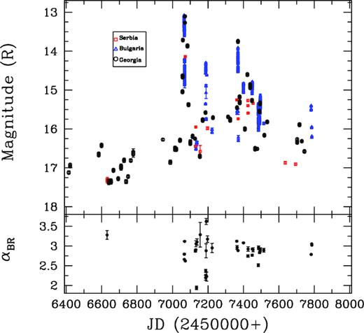
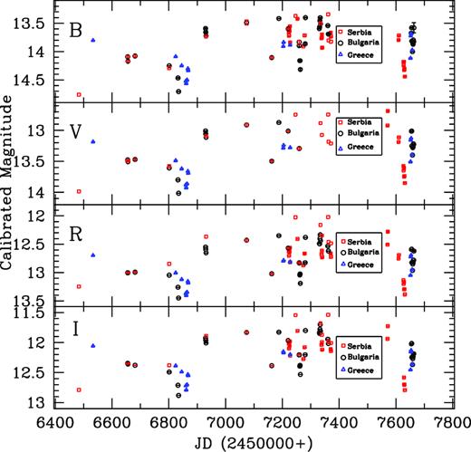
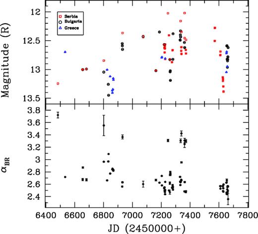
The LTV LC of 3C 66A is shown in Fig. 1 for a total of 295 nights over nearly 4 yr from 2013 January to 2017 January. The B, V, R, and I LCs are shown from top to bottom panels. We observed this source on 130 nights for a total of 697 photometric frames with maximum sampling in V and R bands. We averaged the magnitudes on the daily basis to understand the long-term behaviour of the source. We also used the archival data of the Steward Observatory (Smith 2009) available online for V band for 165 nights. In order to visualize the nature of variability more clearly, we plot the R-band LC in the upper panel of Fig. 2. It can be seen that the R-band LC shows many small subflares superimposed on the long-term trends. First, there is a decaying trend in the LC from JD 6400 to JD 6830 where the magnitude drops by 0.62. There is one major outburst during JD 6830–7370, peaking at around JD = 7200 with R = 14.07. The source magnitude changes by 0.64 from mR = 14.7 to 14.1 and back again during this outburst over about 370 d. After that, there is again an overall rising trend during JD 7370–7800 by Δm = 0.53.
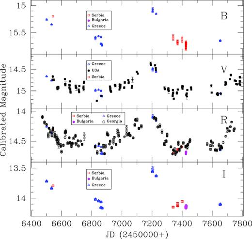
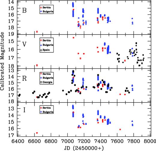
Long-term light curve (LC) of 3C 66A during the period 2013–2017. The top to bottom panels, respectively, show B, V, R, and I calibrated magnitudes and different symbols indicate data from different telescopes as defined in each panel separately.
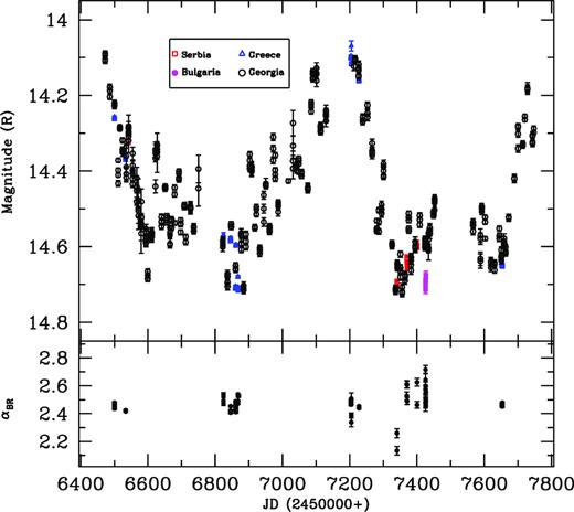
R-band LC of 3C 66A (upper panel) and the variation of spectral indices αBR with respect to JD (lower panel). Spectral indices are calculated for those nights where we have quasi-simultaneous data in B and R bands.
To set some context, 3C 66A exhibited an exceptional outburst around 2007 September, reaching peak brightness at ∼13.4 (Böttcher et al. 2009). Also, Kaur et al. (2017) presented a decade long LC of 3C 66A and found this source reaching a peak brightness of 13.40 in R band on 2010 November 1 with a minimum magnitude of only 15.1 in 2011 August. During our observing campaign, the average R-band magnitude is 14.4 with a maximum of 14.07 mag on JD = 7200 and a minimum of 14.72 mag on JD = 7340. Hence, we can say that the source is mostly in a relatively high state during our observing campaign. LCs in other bands also show similar behaviour. The mean magnitudes in the B, V, and I bands are 15.43, 14.80, and 13.83, respectively. The maximum and minimum brightness magnitudes are in B band: max = 15.07, min = 15.80; inV band: max = 14.36, min = 15.23; and in I band: max = 13.50, min = 14.16. While Fig. 1 makes it clear that we have many fewer data points in the B and I bands, fortuitously, several were taken close to both the minima and greatest maxima.
We searched for a relationship between colour index with respect to magnitude that is needed to ascertain whether flux changes are associated with the spectral changes. We used the simultaneous observed data in B, V, and R bands for a particular night. Fig. 3 shows the colour variability diagram during the period 2013–2017. The colour bar indicates the progression of time in JD (245 0000 +). We have fitted straight lines (CI = m × R + c) to colour index (CI) versus R magnitude plot. We found m = 0.021 ± 0.019; c = 1.30 ± 0.29, with linear Pearson correlation coefficient r = 0.13 indicating p = 0.069. Here a positive correlation is defined as a positive slope between the colour index and magnitude of the blazar that implies that the source tends to be bluer when it brightens or redder when it dims. An opposite correlation with negative slope implies the source follows a redder when brighter behaviour. As the nominal values of the slopes are small and do not exceed twice the errors, we did not find any significant correlation between magnitude and colour index for this blazar. In the previous studies of spectral variability, Böttcher et al. (2005) found a weak positive correlation between (B − R) versus R magnitude when the source was in a low brightness state with R ≥ 14.0 but no clear correlation was found in brighter states of the source. Also, this source was a target of WEBT campaign again in 2007–2008 when it was in a high optical state, reaching a peak brightness of R ∼ 13.4 but then it did not display spectral variability (Böttcher et al. 2009).
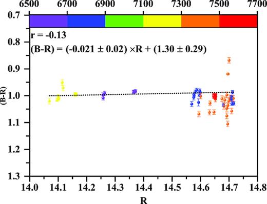
Colour versus magnitude relation for 3C 66A.
3.1.2 Spectral energy distribution
To learn about the origin of variability on longer time-scales, we studied the SED in optical bands in different flux states. We adopted the assumption by Hagen-Thorn et al. (2004) (and considered later by Larionov et al. 2008, 2010) that the flux changes over the relevant set of observations arise from a single variable source (or multiple sources with similar SED). Hence, if the relative SEDs do not change and the variability is caused only by flux variations in that source region, then if n is the number of bands in which observations are made, the measured points should lie on straight lines in the n-dimensional flux density space. As noted by Larionov et al. (2010), the converse would also be true, so that an observed linear relation between flux densities at two different wavelengths while the brightness varied means that the flux ratio, or slope is invariant. If linear relations were detected between multiple bands that would mean that the slopes of those lines could yield the constant relative SED of that variable source component.
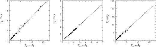
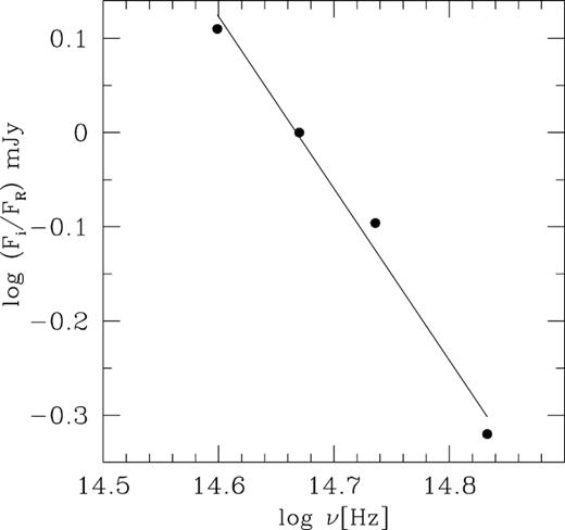
Hence we searched for the flux–flux relations between the B, V, R, and I bands. First, we transformed magnitudes into dereddened flux densities using the Galactic absorption from Schlegel, Finkbeiner & Davis (1998); see also Bessell, Castelli & Plez (1998). The flux–flux relations are shown in Fig. 4. it can be seen from the figure that flux ratios follow linear dependencies, and we used R-band data to obtain relations as Fi = ci + miFR, where i = B, V, and I bands. These linear regressions are used to construct the SED during different flux states of the source observed during our campaign, i.e. maximum (7.75 mJy), average (4.76 mJy), and minimum (3.68 mJy) fluxes. All the three curves are fitted with a power law, i.e. Fν ∝ ν−α, for the spectral index α. Spectral indices for all the mentioned flux states are provided in the upper part of Table 2 and are constant at ≃1.66. As mentioned above, slopes of the linear regressions can also be used to construct the relative SED of the variable source. The values of these slopes and the number of observational points used in producing them are provided in Table 3. A SED of 3C 66A that is normalized to the R band is shown in Fig. 5. We derive a power-law slope of the variable component to be α = 1.60 ± 0.09. As long as we can assume that additional components are responsible for the observed variability and the relative SED of this variable portion is not varying, it can be concluded that the origin of variability of this blazar is intrinsic. It then can be accommodated within a non-thermal variable component that has a continuous injection of relativistic electrons with a power-law energy distribution of p ≃ 4.3 as α ≃ (p − 1)/2.
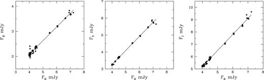
Flux–flux dependence of 3C 66A, where the B (left), V (centre), and I (right) band fluxes are plotted against the R flux; lines represent linear regressions.
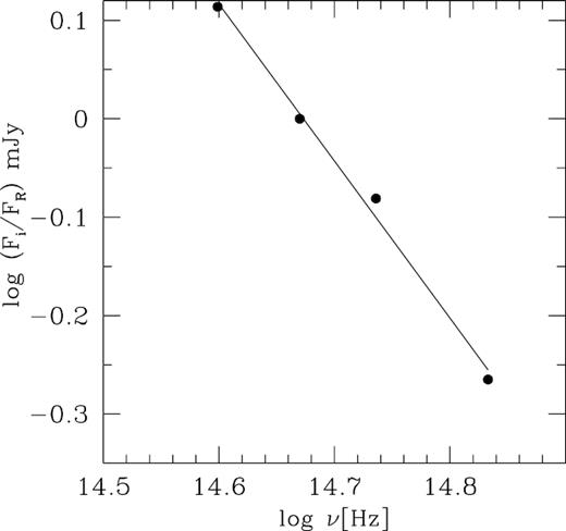
Relative SED of the variable component of 3C 66A, normalized with respect to R band.
Spectral indices of 3C 66A and S4 0954+658 for various flux states.
| Source | Flux (mJy) | Spectral index |
|---|---|---|
| 3C 66A | 7.75 | 1.64 |
| 4.76 | 1.66 | |
| 3.68 | 1.68 | |
| S4 0954+658 | 18.01 | 1.84 |
| 4.31 | 1.90 | |
| 0.34 | 2.72 |
| Source | Flux (mJy) | Spectral index |
|---|---|---|
| 3C 66A | 7.75 | 1.64 |
| 4.76 | 1.66 | |
| 3.68 | 1.68 | |
| S4 0954+658 | 18.01 | 1.84 |
| 4.31 | 1.90 | |
| 0.34 | 2.72 |
Properties of variable emission components of 3C 66A and S4 0954+658.
| Source | Band | Number of observations | log (m) |
|---|---|---|---|
| 3C 66A | I | 65 | +0.114 |
| R | – | ||
| V | 66 | −0.081 | |
| B | 65 | −0.265 | |
| S4 0954+658 | I | 43 | +0.110 |
| R | – | – | |
| V | 26 | −0.096 | |
| B | 38 | −0.320 |
| Source | Band | Number of observations | log (m) |
|---|---|---|---|
| 3C 66A | I | 65 | +0.114 |
| R | – | ||
| V | 66 | −0.081 | |
| B | 65 | −0.265 | |
| S4 0954+658 | I | 43 | +0.110 |
| R | – | – | |
| V | 26 | −0.096 | |
| B | 38 | −0.320 |
3.2 S4 0954+658
S4 0954+658 is a BL Lac object with a claimed redshift of z = 0.367 (Stickel, Fried & Kuehr 1993); however, Landoni et al. (2015) found a featureless spectrum and a limit of z > 0.45, which is based on non-detection of the host galaxy. This source is optically active and its optical variability was first studied by Wagner et al. (1993). Raiteri et al. (1999) studied a 4-yr long optical LC and detected fast large amplitude variations. They also found that the variations over long time-scales for this source were not associated with spectral variations. Papadakis et al. (2004) studied intraday flux and spectral variability of this source during 2001–2002. Hagen-Thorn et al. (2015) studied the optical flux and polarization variability of this blazar during 2008–2012. They found flux variations exceeded 2.5 mag and a degree of polarization that reached 40 per cent. Larionov et al. (2011) also performed photopolarimetric observations of S4 0954+658 during 2011 and found it to have been in a faint state in 2011 mid-January with a brightness level R ∼ 17.6, but by the middle of March the optical brightness rose up to ∼14.8 mag, showing flare-like behaviour. During the rise of the flux, the position angle of the optical polarization rotated smoothly over more than 200°. Bachev (2015) presented the intranight monitoring of the blazar during 2015 February and found violent variations on very short time-scales of ∼0.1 mag within ∼10 min.
3.2.1 Long-term flux and colour variability
The LTV LC of S4 0954+658 is shown in Fig. 6 for a total of 170 nights over nearly 4 yr from 2013 February to 2017 June. B, V, R, and I LCs are respectively shown from the top to the bottom panels of the above figure. To understand the long-term behaviour of this source, it was observed for a total of 1756 photometric frames with maximum sampling in V and R bands. In order to visualize the nature of variability more clearly, we replot the R-band LC on an expanded scale in upper panel of Fig. 7; it displays many short subflares superimposed on the longer term trends. The source was in a low optical state during the period MJD 6400–7000, with the mean magnitude of this source during this period is ∼17. After this period, the source flux increased significantly and reached up to an R magnitude of ∼13 as was also reported by Bachev (2015). Until MJD = 7600 this source displayed many flare-like events. There also was a strong flare peaking around MJD = 7810 that was only caught in V-band measurements; it involved a rise of ∼2 mag over ∼100 d and a more rapid decline. During our observing campaign, the faintest R-band magnitude was 17.40 at MJD = 6640 and the brightest was 13.19 mag on MJD = 7070. LCs in other bands also show similar behaviours. The faintest and brightest magnitudes, respectively, in B band were 18.65 and 14.15; in V band, 17.91 and 15.31; and in I band, 16.66 and 12.64. Hence, during our campaign we observed the source in its low state and in its high state.
Long-term LC of S4 0954+658 during the period 2013–2017, with symbols as in Fig. 1.
R-band LC of S4 0954+658 (upper panel) and the variation of spectral indices αBR (lower panel) with respect to JD (lower panel).
In order to search for the relationship between colour index with respect to the magnitude, we used the simultaneous data in B and R bands. A colour variability diagram is shown in Fig. 8 where the colour bar indicates the progression of time in JD(245 0000 +). The straight line fitted to colour index versus R magnitude gives m = 0.048 ± 0.010; c = 0.45 ± 0.21 = 0.337; p = 0.51 that indicates a positive correlation between colour and magnitude. Raiteri et al. (1999) studied the long-term LC of this source and detected large amplitude variations but they were not associated with the spectral variations.
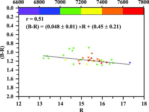
Colour versus magnitude relation of S4 0954+658.
3.2.2 Spectral energy distribution
As we did for 3C 66A, we examined the flux–flux relations of S4 0954+658, shown in Fig. 9, and found that they follow linear regressions. Using the slopes of these linear regressions, we constructed SEDs at maximum (18.01 mJy), average (4.31 mJy), and minimum (0.34 mJy) levels, respectively. We fitted these SEDs using Fν ∝ να and their respective slopes are provided in Table 2. These indicate that the slope is flatter when the flux increases, which is a common property of high-synchrotron-peaked blazars (e.g. Vagnetti, Trevese & Nesci 2003; Hu et al. 2006; Gaur et al. 2012). According to Hagen-Thorn et al. (2004), if such flux–flux relations are linear, a variable emission component is likely to be responsible for the variability. Hence, we constructed the relative SED of the variable emission in Fig. 10 using the slopes of flux–flux relations provided in Table 3. These indicate that the slope of the variable component is 1.82 ± 0.15. Hence, the variability of S4 0954+658 can be interpreted in terms of a non-thermal variable component that has a continuous injection of relativistic electrons with a steep power-law energy distribution of p ∼ 4.64.
Flux–flux dependence of the blazar S4 0954+658, where the B (left), V (centre), and I (right) band fluxes are plotted against the R flux; the lines represent linear regressions.
Relative SED of S4 0954+658, normalized to R band.
3.3 BL Lacertae
BL Lacertae (BL Lac) is a prototype of the blazar class (at the redshift z = 0.069; Miller & Hawley 1977) and is classified as low-frequency-peaked blazar (LBL). BL Lac has long known strong variability in optical bands and is one of the favourite targets of multiwavelength campaigns, such as those carried out by the WEBT/GLAST-AGILE Support Program (GASP; Böttcher et al. 2003; Raiteri et al. 2009, 2010, 2013; Villata et al. 2009, and references therein). It displays intense optical variability on short and intraday time-scales (e.g. Clements & Carini 2001; Gaur et al. 2014; Agarwal & Gupta 2015). It also shows strong polarization variability (Marscher et al. 2008; Gaur et al. 2014, and references therein). In previous studies, it has been found that flux variations are associated with spectral changes (Villata et al. 2002; Papadakis et al. 2003; Hu et al. 2006). Most of the observed properties of this source can be attributed to synchrotron emission from highly relativistic electrons within a helical jet (Raiteri et al. 2009). BL Lac is within a relatively bright host galaxy and we removed its contribution from the observed magnitudes by following the method provided in Gaur et al. (2015a).
3.3.1 Long-term flux and colour variability
The LTV LC of BL Lac is shown in Fig. 11 for a total of 73 nights over nearly 3 yr spanning 2014 through 2016. The source displayed significant flux changes on long-term time-scales in all the bands we measured (B, V, R, and I). The variability amplitudes seen in the B, V, R, and Ibands are 263, 260, 254, and 251 per cent, respectively. The equivalent total changes in magnitudes are ΔB = 1.31, ΔV = 1.28, ΔR = 1.15, and ΔI = 1.12.
Long-term LC of BL Lac during the period 2014–2016; labels as in Fig. 1.
Our entire set of observations can be divided into three seasons. The first observation season covered the period 2014 May 23–2014 September 30, during which BL Lac was observed for a total of 14 nights. The second cycle spanned 2015 February 20–2015 December 14, when the source was observed on 36 nights. The third season covers the period 2016 June 30–2016 October 1, when BL Lac was observed for a total of 23 nights. The magnitude of BL Lac ranged between 13.4 and 12.3 in the Rband during this 3-yr span. In some of the nights, observations were performed using two telescopes and we found good agreement between them. This source was extensively observed in the past by the WEBT collaboration and they found the magnitude to vary between 14.8 and 12.5 in the Rband (Villata et al. 2002, 2004; Raiteri et al. 2010, 2013, and references therein). Hence, we can conclude that we observed BL Lac in a relatively high state, as noted above.
We calculated the spectral index for each night of our observations and they are shown in the lower panel of Fig. 12. The αBR slope is very steep during the observing period and varies between 2.4 and 3.5. This plot again indicates that the emission is dominated by synchrotron emission and shows strong bluer-when-brighter trends.
R-band LC of BL Lac (upper panel) and the variation of spectral indices αBR with respect to JD (lower panel).
A mildly chromatic behaviour is found for the LTV, with a slope of 0.072 ± 0.02, intercept of 0.14 ± 0.21, r = 0.468, p = 3.3e-05 for the (B − R) CI versus Rmagnitudes shown in Fig. 13. This is in accordance with Villata et al. (2004) where they found a similar slope between (B − R) versus Rduring the period 1997–2002; the mildly chromatic long-term variations were simply explained in terms of changes in Doppler factors. Also, it can be seen from Fig. 12 that there are various outbursts superimposed on the long-term trends that vary over time and the chromatism is also variable. The slope of 0.1 should be considered to represent only a mean value.
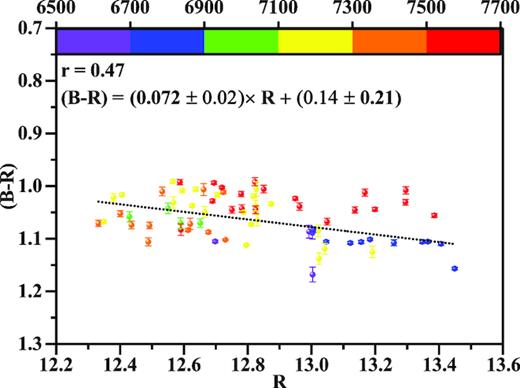
(B − R) colour index versus Rmagnitude of BL Lac on longer time-scales.
It can be seen that the smaller flares/brightness changes on time-scales of days are superimposed on the longer term trends. In previous studies of BL Lac it was argued that much of the variability can be explained by changes in the Doppler factor of the jet emission region (e.g. Villata et al. 2004; Larionov et al. 2010).
3.3.2 Spectral energy distribution
We calculated the flux–flux dependencies for the B, V, R, and Ibands and these are shown in Fig. 14. The relations are not very well fit by linear functions and hence the spectra are far from power laws. So we fit them with second-order polynomials, i.e. a + b × F + c × F2. We then produced continuum spectra of BL Lac by using these polynomial regressions and these are shown in Fig. 15 for R-band fluxes of 15, 25, and 35 mJy, which are within the range of our measurements.
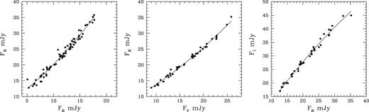
Flux–flux dependence of the BL Lac, where the Rflux is plotted against the B(left), V(centre), and I(right) band fluxes. The lines represent second-order polynomial regressions.

Spectra of BL Lac in optical bands obtained from polynomial regressions. Black, blue, and red curves connecting the I, R, V, and Bbands represent the spectra for 35, 25, and 15 mJy, respectively. The blue and red arrows and the corresponding curves connecting them represent the spectra obtained from the 35 mJy spectrum corresponding to decreasing δ by a factor of 1.19 for p = 3 (blue) or by a factor of 1.25 for p = 2 (red). Details are in the text.
If the intrinsic spectrum is a power law, Fν ∝ να and α is taken as independent of wavelength over this modest range, then the flux–flux plots would have shown linear dependencies; however, this is not quite the case in our observations as shown in Fig. 14. Following Larionov et al. (2010), if we assume that the flux variations arise from changes in the viewing angle that lead to changes in the Doppler factor, δ, then in the observer’s rest frame, the flux density is |$F_{\nu } = \delta ^{p} F_{\nu }^{\prime }$| (Rybicki & Lightman 1979; Urry & Padovani 1995), where primed quantities refer to the source rest frame, p = 3 for the situation where the radiation comes from a moving source with a compact emission zone (shock/knot), while p = 2 is appropriate for a smooth continuous jet (Begelman et al. 1994). Also, the frequencies are affected by the Doppler shift as ν = δν′. Hence, in Fig. 15, a logarithmic plot, the variation in the Doppler factor by Δ log δ leads to a shift in flux and in frequency in the following form: Δlog Fν = pΔ log δ and Δlog ν = Δ log δ. Here, we calculate the shift in the Doppler factor that is required to obtain the spectrum corresponding to 15 mJy from the highest flux spectrum of 35 mJy. We can roughly reproduce (as shown by the coloured lines in Fig. 15) the lower spectrum from the higher one by lowering δ by a factor of 1.19 for p = 3 or by a factor of 1.25 assuming p = 2, but given the very modest curvature over our limited range of bands, we cannot really distinguish between these possibilities. Hence, the most plausible explanation to describe the overall flux and colour variability during 2013–2017 is in terms of modest Doppler factor variations that affect the observed radiation coming from a jet. However, due to the limited range of frequencies, we cannot completely ruled out the possibility of other variability models.
Larionov et al. (2010) found a somewhat larger shift in the Doppler factor by a factor of 1.58 with p = 3 to fit a wider range of flux variations in data taken between 2000 and 2008. Because they had measurements in more infrared bands they argued that they could distinguish between the shock/knot and smooth jet possibilities and favoured the former.
4 DISCUSSION AND CONCLUSIONS
We have presented the results of photometric monitoring of three TeV blazars, namely 3C 66A, S4 0954+658, and BL Lac, over nearly 4 yr in 2013–2017 for a total of 536 nights in B, V, R, and Ibands. We studied their flux and spectral variability on these long time-scales. All three sources showed significant variability during our observing runs with the maximum variability shown by S4 0954+658 (ΔR ∼ 4). BL Lac revealed a more moderate variation of around ΔR ∼ 1.12, while weaker variations of ΔR ∼ 0.65 were displayed by 3C 66A. Comparison of our photometric observations with the earlier observations of same sources indicates that we observed the blazars 3C 66A and BL Lac in high states. However, the blazar S4 0954+658 was observed in low and high states. This source underwent many strong flares during our observations and reached a maximum brightness of around ∼13 mag in 2015 February.
We also studied the correlation between Rmagnitude and the colour indices. We did not find any correlation for 3C 66A, but found weak positive correlations for S4 0954+658 and BL Lac. It can be seen that the spectra of S4 0954+658 are getting flatter as the flux increases (Table 2) that indicates a bluer-when-brighter trend. For BL Lac, we found a positive slope of 0.1 between the (B − R) colour index and Rmagnitude, again indicating a similar trend, which is commonly seen for LBL blazars. Bluer-when-brighter chromatism can be explained with a one-component synchrotron model in that the more intense the energy release, the higher the typical particle’s energy and the higher the corresponding frequency (Fiorucci, Ciprini & Tosti 2004). It can also be result from the injection of fresh electrons with an energy distribution harder than that of the previously cooled ones (e.g. Kirk et al. 1998; Mastichiadis & Kirk 2002). The long-term trends we saw are generally mildly chromatic. The flatter slope of the colour–magnitude diagram could be revealing the presence of multiple variable components, each evolving differently. Hence, superposition of different spectral slopes from multiple components leads to a general reduction of the colour–magnitude correlations (Bonning et al. 2012; Bachev 2015). It has been found in previous studies that the slope of the optical spectrum is often only weakly sensitive to the long-term trends, while strictly following the bluer when brighter trends on short time-scales (Villata et al. 2002; Larionov et al. 2010; Gaur et al. 2012, 2015a).
IDV of two of these sources, S4 0954+658 and BL Lac, was investigated in Bachev (2015) and Gaur et al. (2017), respectively. S4 0954+658 was observed by Bachev (2015) during its unprecedented high state in 2015 February when it reached a maximum brightness of ∼13 mag. Rapid, violent variations of 0.1–0.2 mag h−1 were observed on intraday time-scales and favour a geometrical scenario to account for this variability. The IDV of BL Lac was observed by Gaur et al. (2017) over a total of 45 nights and they found strong variability of ∼0.1 mag over a few hours on several nights. The IDV of BL Lac can be associated with models based on shocks moving through a turbulent plasma jet.
Models that have been proposed to explain optical variability of blazars generally involve one or more of the following processes: changes in the electron energy density distribution of the relativistic particles producing variable synchrotron emission; inhomogeneities in magnetic fields; shocks accelerating particles in the bulk relativistic plasma jet; turbulence behind an outgoing shock in a jet; and irregularities in the jet flows (e.g. Marscher, Gear & Travis 1992; Giannios et al. 2009; Gaur et al. 2014; Marscher 2014; Calafut & Wiita 2015; Pollack et al. 2016). The flux variations in blazars on longer time-scales can also be explained by the launching of new components (or shocks) (e.g. Marscher & Gear 1985; Hughes, Aller & Aller 1989) or mechanisms involving geometrical effects such as modestly swinging jets, for which the path of the relativistically moving source regions along the jet deviates a bit from the line of sight, leading to a changing Doppler factor (e.g. Gopal-Krishna & Wiita 1992; Pollack et al. 2016) or in a helical jet model where the orientation changes though the rotation about the helix (Villata et al. 2009).
In order to try to understand the origin of variability of these blazars during our observations, we studied flux–flux relations of these sources, based on the assumption that linear relations between observed fluxes at different wavelengths suggest that the slope does not change during the period of flux variability. And, if the variability arises from a single variable source (or multiple components with similar SEDs), then its slope can be derived from the slopes of the flux–flux relations. Hence, we calculated the flux–flux relations of these three blazars and found that those of 3C 66A and S4 0954+658 followed linear regressions. Hence, a single variable source (or multiple components with similar SEDs) is probably responsible for the variability we are seeing. Using the slopes of the flux–flux relations, we constructed the relative SED of this variable components. The slopes of the variable emitting region of 3C 66A and S4 0954+658 are found to be ≃1.65 and 1.8, respectively. Hence, using the flux–flux relations, we suggest that the variability in these two sources can be interpreted in terms of a non-thermal variable component that has a continuous injection of relativistic electrons with a power-law energy distributions around 4.3 and 4.6, respectively.
The flux–flux relations of BL Lac are better fitted with a second-order polynomial that implies that the observed flux variations more likely arise from the changes in the Doppler factor of the relativistic jet, as suggested earlier (Villata et al. 2002; Larionov et al. 2010, and references therein). Hence, we calculated the optical spectra of BL Lac at different flux states between 15 and 35 mJy. We found that the lowest spectrum could be reasonably reproduced from the highest flux spectrum by decreasing the Doppler factor by a factor of ∼1.2. These observations of long-term flux and mildly achromatic BL Lac variability might be explained to arise from changes in the viewing angle, which lead to the Doppler factor becoming variable (Larionov et al. 2010 and references therein).
Our observations of these three blazars allow us to make plausible inferences about the origins of variability in optical bands. However, as we are dealing with very narrow range of frequencies in the optical SEDs and we have limited data set that is simultaneous in B, V, R, and Ibands needed to properly study flux–flux relations, the conclusions must be used with caution. Even larger data sets and broader multiwavelength modelling of SEDs are required to firmly constrain various blazar jet parameters.
SUPPORTING INFORMATION
Table 1. Observation log of optical photometric observations of the blazar 3C 66A.
Please note: Oxford University Press is not responsible for the content or functionality of any supporting materials supplied by the authors. Any queries (other than missing material) should be directed to the corresponding author for the article.
ACKNOWLEDGEMENTS
We would like to thanks the anonymous reviewer for the constructive comments that helped us to improve the paper scientifically. HG acknowledges the financial support from the Department of Science and Technology, India, through INSPIRE faculty award IFA17-PH197 at ARIES, Nainital. This research was partially supported by the Bulgarian National Science Fund of the Ministry of Education and Science under grants DN 08-1/2016, DM 08-2/2016, DN 18-13/2017, DN 18-10/2017, and KP-06-H28/3 (2018) and by the project RD-08-112/2018 of the University of Shumen. The authors thank the Director of Skinakas Observatory Professor I. Papamastorakis and Professor I. Papadakis for the award of telescope time. The Skinakas Observatory is a collaborative project of the University of Crete, the Foundation for Research and Technology – Hellas, and the Max-Planck-Institut für Extraterrestrische Physik. The Abastumani team acknowledges financial support by the Shota Rustaveli National Science Foundation of Georgia under contract FR/217554/16. GD and OV gratefully acknowledge the observing grant support from the Institute of Astronomy and Rozhen National Astronomical Observatory, Bulgarian Academy of Sciences, via bilateral joint research project ‘Observations of ICRF Radio-Sources Visible in Optical Domain’. This work is a part of the Projects No. 176011 (‘Dynamics and Kinematics of Celestial Bodies and Systems’), No. 176004 (‘Stellar Physics’), and No. 176021 (‘Visible and Invisible Matter in Nearby Galaxies: Theory and Observations’) supported by the Ministry of Education, Science and Technological Development of the Republic of Serbia. Observations obtained by the FERMI/Steward Observatory blazar monitoring program have been funded through NASA/Fermi Guest Investigator grant NNX08AW56G, NNX09AU10G, NNX12AO93G, and NNX15AU81G.
Footnotes
iraf is distributed by the National Optical Astronomy Observatories, which are operated by the Association of Universities for Research in Astronomy, Inc., under cooperative agreement with the National Science Foundation.
Dominion Astrophysical Observatory Photometry software.
