


Abstract
Using cosmological particle hydrodynamical simulations and uniform ultraviolet backgrounds, we compare Lyman-α forest flux spectra predicted by the conventional cold dark matter (CDM) model, the free-particle wave dark matter (FPψDM) model, and extreme-axion wave dark matter (EAψDM) models of different initial axion field angles but with a fixed boson mass mb ∼ 10−22 eV against the BOSS Lyman-α forest absorption spectrum. We recover results reported previously that the CDM model agrees better with the BOSS data than the FPψDM model by a large margin, and we find that the difference of total χ2’s is 120 for 420 data bins. These previous results demand a larger boson mass by a factor >10 to be consistent with the date and are in tension with the favoured value determined from local satellite galaxies. We however find that such tension is alleviated as some EAψDM models predict Lyman-α flux spectra agreeing better with the BOSS data than the CDM model, and the difference of total χ2’s can be as large as 24 for the same bin number. We stress that our results are obtained based on optimization of a limited set of parameters with others fixed to a well-known heating model as priors; hence, the results are not fully optimized and should be taken as a strong indicator.
1 INTRODUCTION
The remarkable success of lambda cold dark matter model (ΛCDM) is a milestone in modern cosmology. Although the nature of dark energy and dark matter are still unknown, ΛCDM has been amply tested on many large-scale phenomena successfully, such as cosmic microwave background (CMB) fluctuations (Planck Collaboration XIII 2016), baryon acoustic oscillations (Eisenstein et al. 2007), accelerating expansion of the universe (Riess et al. 1998; Perlmutter et al. 1999), etc. Despite that, predictions of ΛCDM have however been in tension with observations on small scales (≲10 kpc). One well-known example is the missing satellites problem (Klypin et al. 1999); a related problem is the too-big-to-fail problem (Boylan-Kolchin, Bullock & Kaplinghat 2011); inside the dwarf spheroidal galaxies, there is a long-debated core-cusp problem (Moore 1994). This small-scale observational evidence casts doubt on the viability of the conventional particle cold dark matter (CDM) model.
Fuzzy dark matter (Hu, Barkana & Gruzinov 2000) or wave dark matter (ψDM; Schive, Chiueh & Broadhurst 2014a) on the other hand provides a viable alternative solution to the small-scale problem (Marsh 2016). The hypothesis made for ψDM is that dark matter consists of extremely light bosons, mb ∼ 10−22 eV. As mb is so small, quantum pressure arising from the uncertainty principle becomes manifestly effective on scales smaller than 10 kpc and impacts on the cosmic structure, where small sub-haloes are suppressed and cores of medium-sized sub-haloes smoothed.
The wave dark matter model also has strong predictive power. It predicts that the first galaxy should form around |$z$| = 12, the galaxy number count should be abruptly diminished beyond |$z$| > 9, and the cosmic reionization occurs late (Schive et al. 2016). Some evidences for the suppression of very high-redshift galaxies from magnification bias have recently been found (Leung et al. 2018), and the relatively late reionization found by Planck (Planck Collaboration XIII 2016) is also consistent with the predictions. It also asserts every galactic halo of any mass should host one and only one stable high-density dark matter core (dubbed the soliton) and the mass of the soliton is strongly correlated with the mass of the halo (Schive et al. 2014b; Veltmaat, Niemeyer & Schwabe 2018). The halo is composed of large-amplitude granules of roughly the same size fluctuating with roughly the same correlation time (Lin et al. 2018). The soliton can robustly survive even in the presence of more massive baryons often found in the inner halo of a galaxy (Chan et al. 2018), and can create detectable signatures in the core of Milky Way through pulsar timing (De Martino et al. 2017).
Despite the initial success, wave dark matter has recently faced a serious challenge from the Lyman-α (Lyα) forest observations (Armengaud et al. 2017; Iršič et al. 2017b). Models with boson masses of 1 to few 10−22 eV determined by the soliton cores of satellite galaxies (Schive et al. 2014a; Chen, Schive & Chiueh 2017) cannot reproduce the observed Lyα flux power spectrum; at least one order of magnitude higher boson mass is required to be consistent with the observations. Not unlike warm dark matter, this challenge renders the wave dark matter model as an inconsistent model requiring a lower particle mass to be consistent with local satellite galaxy observations but at least a 10 times higher particle mass for high-redshift Lyα forest observations.
Recent theoretical developments have however discovered a possible solution for the dilemma faced by wave dark matter (Zhang & Chiueh 2017a,b) in the context of axion-like particles (Hui et al. 2017). Having a capability to change the linear matter power spectrum shape, to which the Lyα power flux spectrum is most sensitive, this class of wave dark matter models, motivated by the QCD axion mechanism and called the extreme axion wave dark matter model (EAψDM), can provide a unique degree of freedom imprinted in the linear matter power spectrum not available to cold, warm or interacting particle dark matter models.
The axion model has a field potential |$V = m_b^2f^2(1 - \cos \theta)$|, where f is the axion decay constant or the axion symmetric breaking scale and θ is the axion angle. The axion potential becomes a simple harmonic oscillator when θ → 0, and we call this limit the free-particle ψDM (or FPψDM). (In the non-relativistic limit, |$m_b^2f^2\langle 2\theta ^2\rangle$| is the conventional mass density, where 〈...〉 is a short-time average to filter out the Zitterbewegung of rapid harmonic oscillation.) Due to the Hubble friction experienced by the axion field, any finite-amplitude initial θ will always approach this small-amplitude limit at a late time. If the initial θ is not only of finite amplitude but also very close to π, the unstable equilibrium, the angle θ will stay near the unstable equilibrium for a relatively long time, causing a delay in the non-linear oscillation and producing parametric instabilities in the perturbation (Zhang & Chiueh 2017b). This parametric instability results in a spectral bump slightly below the high-k cut-off first identified in Zhang & Chiueh (2017a); the spectral bump was later confirmed in Cedeño, González-Morales & Ureña-López (2017).
EAψDM can eventually become FPψDM in the matter-dominant era described by the Schroedinger-Poisson equation (with Re[ψ] and Im[ψ] to be identified as cosine and sine components of the Zitterbewegun oscillation, respectively); but EAψDM can have a different linear matter power spectrum from that of FPψDM, as the final spectrum depends on the spectral formation history mostly prior to the radiation-matter equality. This difference in the linear matter spectrum can significantly alter the predicted Lyα flux power spectrum. In this paper, we focus on testing the EAψDM model against the Lyα flux power spectra obtained from the BOSS survey (Palanque-Delabrouille et al. 2013), and conclude that in some narrow range of initial angle of θ, the trouble faced by the wave dark matter can be alleviated.
This paper is organized as follows. In Section 2, we describe our simulations. We analyse the matter power spectra and compare flux power spectra with the BOSS Lyα data (Palanque-Delabrouille et al. 2013) in Section 3. In Section 4, we discuss our findings in the comparisons with the BOSS data. Finally, we present our conclusion in Section 5. Appendix A describes the splicing method. Appendix B shows the convergence test of flux power spectrum. We also present a comparison of representative Lyα spectra of different models in Appendix C. Appedix D shows details of Lyα flux power spectra. The suffixes ‘c’ in length scales refer to units in the co-moving coordinate.
2 METHODOLOGY
2.1 Power spectra
One of the common features of wave dark matter power spectra is the suppression of small-scale structures below the Compton length prior to the matter-radiation equality (Hu et al. 2000; Zhang & Chiueh 2017a) and the existence of a Jeans length due to the uncertainty principle in the matter dominant era (Woo & Chiueh 2009). The EAψDM power spectra, however, have one more degree of freedom other than the boson mass mb, the initial misaligned field angle θ, which gives rise to a broad spectral bump immediately longward of the spectral suppression (see Fig. 1). The bump and suppression features are best shown in the ψDM-to-CDM transfer function, |$T^{2}_{\psi \rm DM}(k, z) = P_{\psi \rm DM}(k, z)/P_{\rm CDM}(k, z)$|, where P is the matter power spectrum. Although |$T^{2}_{\psi \rm DM}(k, z)$| generally depends on redshifts, Zhang & Chiueh (2017b) showed that the dependence of the CDM-to-ψDM transfer function on redshift |$z$| is extremely weak in the wavenumber regime probed by Lyα observations (k ≲ 5.9 h Mpcc−1). Specifically, a recent study (Armengaud et al. 2017) discussed that the quantum pressure influence on the ψDM dynamics at wavenumbers probed by Lyα forest observations could be neglected in the particle mass range m22(≡mb/10−22 eV) ≳ 1.1.
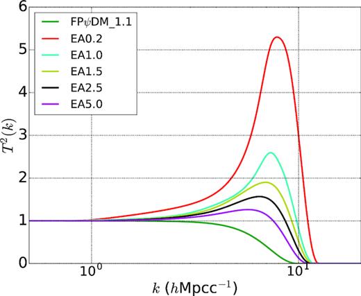
ψDM-to-CDM transfer functions for FPψDM, EA0.2, EA1, EA 1.5, EA 2.5, and EA 5.0 at z = 49 with m22 = 1.1. Note that all ψDM models have strong spectral suppression at high k, but only EAψDM models have broad spectral bumps.
To set the stage for this investigation, we show in Fig. 1 the transfer functions |$T^{2}_{\psi \rm DM}$| of FPψDM, EAψDM with δθ(≡π − θ) = 0.2°, 1°, 1.5°, 2.5°, and 5° at |$z$| = 49. (Hereafter, we refer to EAψDM, for example, with δ = 0.2° as EA0.2.) From Fig. 1, it is clear that the smaller the δθ the larger the cut-off wavenumbers kc (defined by T(kc) = 0.5). These EAψDM models have spectral bumps immediately longward of the cut-off, suggesting that the halo assembly history in EAψDM can significantly deviate from the traditional CDM and the FPψDM predictions at high redshifts (Schive & Chiueh 2018). Therefore, the Lyα forest measured in the redshift range |$z$| ∼ 2–4 can impose constraints on the particle mass and the initial field angle of EAψDM.
In fact, the Lyα flux power spectrum is affected by the cut-off kc of the linear matter power spectrum even more sensitively than the non-linear matter power spectrum at |$z$| ∼ 2–4. The former probes an intermediate gas density up to unity optical depth and is thus sensitive to the cosmic web, a structure in the relatively weakly non-linear regime. By contrast, the matter power spectrum is dominantly contributed by the highly non-linear collapsed haloes. In this regard, the quasar flux spectrum is less affected by non-linear evolution and capable of capturing the linear matter power spectrum.
2.2 Hydrodynamical simulations
Accurately simulating ψDM dynamics needs to solve the Schrödinger-Poisson equation (e.g. Schive et al. 2014a,b). However, such simulations in large (∼(100 h−1Mpcc)3) simulation boxes with sufficiently high (∼100 h−1pcc) resolution are prohibitively computationally expensive even with the most advanced supercomputers. This is due primarily to that the time-step of computation scales unfavourably with the squared grid size in a zoom-in calculation in order to capture quantum pressure inside collapsed haloes. Hence, it is reasonable to inquire under what conditions CDM-hydro simulations with the initial matter power spectrum modified to the ψDM spectrum can still capture the Lyα forest in the ψDM scenario. It turns out that the relatively low-resolution dynamical range of the BOSS data (Palanque-Delabrouille et al. 2013) can validate this approach. (See Section 3.1 for details.)
By contrast, high-resolution observations, such as the XQ-100 (Iršič et al. 2017c) and HIRES/MIKE (Vogt et al. 1994; Bernstein et al. 2002), measure spatial scales down to 100 h−1kpcc, a scale that is well within the quantum suppression regime for mb ∼ 10−22 eV, and hence CDM-hydro simulations are not valid. Even for CDM, such high-resolution simulations are technically very challenging. (See Lukić et al. 2015, which discussed high-accuracy Lyα forest simulations of the CDM model.) In an attempt to solve the quantum pressure problem for high-resolution simulations, a modified CDM-hydro code (ax-gadget) has been developed, where a quantum force law has been implemented in every fluid element (Li, Hui & Bryan 2018; Nori & Baldi 2018; Nori et al. 2019). However, it remains to be seen to what extent such a modified hydro scheme can capture interference patterns upon wave reflection.
Various previous works have adopted the CDM-hydro approach with a modified matter spectrum to approximate wave dark matter dynamics. Schive et al. (2016) pointed out that the growth rate ratio between ψDM and CDM, defined in equation (4) of Schive et al. (2016) for m22 = 1.6, is almost unity for k ≤ 11 hMpcc−1. Using a particle-mesh scheme, Veltmaat & Niemeyer (2016) showed that the quantum pressure effect is not apparent for FPψDM matter power spectrum until k ≳ 150 h Mpcc−1 for m22 = 2.5. Iršič et al. (2017b) used CDM-hydro simulations to address the XQ-100 high-resolution Lyα forest for constraining the boson mass mb. Armengaud et al. (2017) also suggested that quantum pressure is likely negligible for Lyα forest simulations with mb ≳ 10−22 eV. The conclusions of these works are consistent with the approach we adopt. For these very reasons, we shall be contented with the low-resolution BOSS data with CDM-hydro simulation predictions.
In this work, we perform N-body hydro simulations to represent ψDM dynamics. The simulation uses the mesh-free hydrodynamic simulation code, gizmo (Hopkins 2015), which adopts the Lagrangian meshless finite mass (MFM) algorithm. Comparing with the traditional SPH method, MFM has many advantages. The most noticeable of all is that MFM does not require artificial viscosity, an infamous feature adopted by the SPH method to make computation stable. We use the music code (Hahn & Abel 2011) to generate the initial conditions at |$z$| = 49 with the second-order Lagrangian perturbation theory method. The CDM power spectrum is generated by the camb package (Lewis & Bridle 2002), the FPψDM transfer function is generated by the axioncamb (Hložek et al. 2017), and for EAψDM transfer functions we follow the work of Zhang & Chiueh (2017b). The chemistry and cooling library grackle 1(Smith et al. 2017) is used to solve the radiative processes. Also, all linear matter power spectra are computed by genpk (Bird 2017).
To capture the signal of the 1D flux power spectrum from small to large scales, we perform three simulations with (L, N) = (25 h−1 Mpcc, 2 × 5123), (25 h−1 Mpcc, 2 × 1283) and (100 h−1 Mpcc, 2 × 5123), where L3 is the co-moving volume of the simulation box and N is the total number of all particles (dark matter and gas). We apply a simple star formation criterion – gas particles satisfying temperature T < 105 K and overdensity Δ > 1000 are transformed to collisionless stars (Viel, Haehnelt & Springel 2004, 2010). We do not consider metal cooling because the metal abundance in IGM is negligible. The gravitational softening length for three different species (dark matter, gas, and stars) are the same, set to 1/25 of the mean co-moving interparticle distance of dark matter particles. The kernel of MFM is cubic spline and the effective neighbour of the kernel is 32. In all simulations, the primordial helium mass fraction is Y = 0.24. This set of parameters is the same as most previous works on the Lyα flux power spectrum (e.g. Borde et al. 2014; Palanque-Delabrouille et al. 2015; Bolton et al. 2017).
In focusing on the difference produced by different initial matter power spectra of CDM, FPψDM, and EAψDM, we perform all simulations with identical Gaussian random seeds, cosmological parameters, and ultraviolet background (UVB). The adopted cosmological parameters are the best-fitting result for the CDM model suggested by Palanque-Delabrouille et al. (2015), where Ωm = 0.292, Ωb = 0.050, σ8 = 0.858, h = 0.668, ns = 0.929, which are fixed for all dark matter models. We also fix the ψDM mass parameter m22 = 1.1 and adiabatic index γ = 1.5. We use the homogeneous intergalactic UV background of Haardt & Madau (2012), assuming that the intergalactic gas is highly ionized, in ionization equilibrium and optically thin for photoionization and photoheating. We also follow a modification introduced by Bolton et al. (2017), the Sherwood simulation, to the HeII photoheating rate to ensure that the IGM temperature in simulations is in agreement with the IGM temperature estimated from observations (e.g. Becker et al. 2011). The modification adopts |$\epsilon _{\rm He II} = 1.7\epsilon _{\rm He II}^{\rm HM12}$| from |$z$| = 2.2 to |$z$| = 3.4. This boosting factor can be regarded as an approximation method (Theuns et al. 1998) to radiative transfer and non-equilibrium effects during He ii reionization (Puchwein et al. 2015). In low-density regions, the gas density and temperature are closely related, where the thermal behaviour of gas is dominated by adiabatic expansion cooling and photoionization heating. The density–temperature relation for low-density gases can roughly be expressed by a redshift-dependent power law, T(|$z$|) = T0(|$z$|)Δγ(|$z$|) −1 with Δ ∼ 0.3–1, where T0 is the mean temperature of low-density IGM and Δ = ρ/〈ρ〉 is the gas density over the background gas density.
In this work, we find T0(|$z$| = 3.0) ≃ 12 500 K for all simulations, consistent with the simulation work of Bolton et al. (2017). In detail, Fig. 2 depicts our T0(|$z$|) of CDM and EA2.5 simulations compared with the indirect temperature measurement assuming γ ∼ 1.5 and γ = 1.3 for equilibrium ionization (Becker et al. 2011) and γ ∼ 1.5 for non-equilibrium ionization (Puchwein et al. 2015). In fact, Becker et al. (2011) empirically identified a unique temperature proxy |$T(\bar{\Delta }(z), z)$| with simulations, for which |$\bar{\Delta }$| is some characteristic density ranging within 1.2–5.7, depending on redshifts but insensitive to γ; they found that both |$T(\bar{\Delta }(z), z)$| and |$\bar{\Delta }$| can simultaneously be determined by the measured Lyα flux signal without the need to assume γ. We therefore also plot |$T(\bar{\Delta }(z), z)$| of our simulations in Fig. 2 to directly confront their measured |$T(\bar{\Delta }(z), z)$|. Here |$\bar{\Delta }(z)$| is taken from fig. 7 of Becker et al. (2011). Our T0 is related to |$T(\bar{\Delta })$| by |$T_{0} = T(\bar{\Delta })/\bar{\Delta }^{1-\gamma }$| with γ ∼ 1.5 (cf. Fig. 3) determined by a procedure given by Puchwein et al. (2015). Both CDM and EAψDM simulations yield almost identical T0(|$z$|) and |$T(\bar{\Delta }(z), z)$|. Fig. 2 shows that simulated temperatures agree reasonably well with respective measured temperatures, justifying our heating model. (See, however, Sections 4 and 5 for discussions of the possible need of fine-tuning in both local and global heating.)
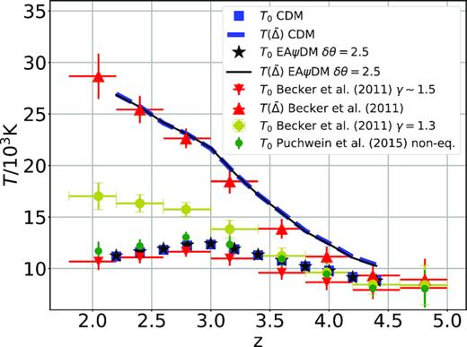
T0(|$z$|) and |$T(\bar{\Delta })$| of the (25 h−1 Mpcc, 2 × 5123) CDM and EA2.5 simulations in comparison with respective measured temperatures. While T0 depends on the assumed γ, |$T(\bar{\Delta })$| can be directly determined by Lyα measurements. Our determination of T0 and |$T(\bar{\Delta })$| follows Puchwein et al. (2015) and Becker et al. (2011). The two measured T0(|$z$|)’s are determined using the same Lyα data calibrated by simulations of non-equilibrium ionization for γ ∼ 1.5 (Puchwein et al. 2015) and equilibrium ionization (Becker et al. 2011) for γ ∼ 1.5 and γ = 1.3.
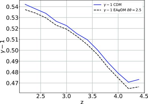
γ(|$z$|) in (25 h−1 Mpcc, 2 × 5123) CDM and EA2.5 simulations.
2.3 Mock Lyman-α forest spectra
2.4 Fitting parameters
The parameter fitting in this work is post-simulation fitting, accounting for uncertainties in simulated Lyman-α signals and measured signals. We consider two categories of fitting parameters in the comparison procedure after the 1D flux power spectrum is obtained. The first category applies different global effective optical depth τeff(|$z$|), defined below, to the simulation flux power spectrum |$P_{\rm F}^{\rm 1D, th} (k)$|. The second category takes into account imperfections of the BOSS data and of simulations.
Astrophysical parameters:
The effective optical depth τeff is related to the photoionization rate in IGM and be normally defined aswhere Fi is the normalized flux at each pixel of sightlines and 〈...〉 the average over all pixels. In most simulation works (e.g. Theuns et al. 1998; Borde et al. 2014; Armengaud et al. 2017; Bolton et al. 2017), τeff is rescaled to follow a power law, τeff(|$z$|) = A(1 + |$z$|)B, where A and B are constants determined from the observational data. In this work, we do not demand τeff(|$z$|) to follow a particular empirical power law, for a reason that parameters A and B are different in different observations (e.g. Meiksin 2009; Becker et al. 2013; Palanque-Delabrouille et al. 2013). As a result, for improving the goodness of fit between the predicted |$P_{\rm F}^{\rm 1D, th} (k)$| and the BOSS data, we choose to independently adjust τeff(|$z$|) at each redshift by rescaling the effective optical depth. The rescaling of τeff can be expressed as(3)\begin{eqnarray*} \tau _{\rm eff}(z) \equiv -\ln (\langle F_{i}\rangle (z)) \end{eqnarray*}with(4)\begin{eqnarray*} \tau _{\rm eff}^{{\prime }}(z) = -\ln (\langle F_{i}^{{\prime }}\rangle (z)), \end{eqnarray*}where |$F^{{\prime }}_{i}$| is the adjusted flux at the ith pixel of spectrum and αeff(|$z$|) is the rescale parameter. This rescaling procedure has been broadly practised and explained in Theuns (2005) and Borde et al. (2014); it is equivalent to globally adjusting the neutral hydrogen density in simulations. In Fig. 4 we show the best-fitting τeff, and they are found to lie between bounds of the empirical fittings of different observations.(5)\begin{eqnarray*} F^{{\prime }}_{i} = F^{\alpha _{\rm eff}}_i = \mathrm{ e}^{-\alpha _{\rm eff}(z)\tau _i}, \end{eqnarray*}- Technical parameters: We next consider the second category of fitting parameters including three factors of technical origins. These factors are contamination of SiI ii and Lyα cross-correlation CSi, imperfection in noise estimate in the BOSS data Cnoise and imperfection of the simulation resolution Creso. The impacts from the three factors to the predicted spectrum are expressed by the following formula:(6)\begin{eqnarray*} P_{\rm F}^{\rm 1D, fit} = P_{\rm F}^{\rm 1D, th} \times (C_{\rm Si}(k, z) \times C_{\rm reso}(k)) + C_{\rm noise}(k, z) \end{eqnarray*}
CSi(k, |$z$|i): Due to the juxtaposition of the two lines, λLyα = 1216 Å and λSiIii = 1206 Å, there is contamination from the SiI ii absorption line to the Lyα absorption line in the observed |$P_{\rm F}^{\rm 1D} (k)$| (McDonald et al. 2006; Palanque-Delabrouille et al. 2013). We adopt a multiplicative term, CSi(k, |$z$|) = (1 + bcos kv)2 + (bsin kv)2 = 1 + b2 + 2bcos kv, to the predicted flux power spectrum first introduced in McDonald et al. (2006) to account for such contamination. Here b = αSi/(1 − 〈F〉(|$z$|)) with αSi being a redshift-independent fitting parameter and |$v$| = 2270 km s−1.
Creso(k): We consider the imperfect resolution of simulation that possibly affects our comparison, and allow for a redshift-independent multiplicative correction factor, Creso(k) = exp (−k2 · αreso), as described in Palanque-Delabrouille et al. (2015), where αreso is a random number obeying a zero-mean Gaussian distribution with a variance σ = 5 and its amplitude is a redshift-independent fitting parameter.
Cnoise(k, |$z$|): The errors of measurement noise estimation need also to be accounted for. Following the method described in Palanque-Delabrouille et al. (2015), we allow for |$\pm 10 {{\ \rm per\ cent}}$| rms errors in the observation noise power spectra at each redshift and include an additive correction term in each redshift bin, Cnoise(k, |$z$|) = Pnoise(k, |$z$|) · αnoise(|$z$|), where αnoise(|$z$|) is a random number obeying a zero-mean Gaussian distribution with a variance σ = 0.1. Again its amplitude is a fitting parameter dependent on redshifts. Here the noise power spectrum Pnoise(k, |$z$|) has been given in the BOSS data.
In total, we have 26 fitting parameters (12 αeff(|$z$|), 12 αnoise(|$z$|), one αSi, and one αreso) for a sample of 420 BOSS data of all redshifts. These fitting parameters are independently adjusted so as to reach a global best fit for each model. We want to stress that, except for τeff(|$z$|), this work follows all remaining 14 fitting parameters formulated in McDonald et al. (2006) and Palanque-Delabrouille et al. (2015).
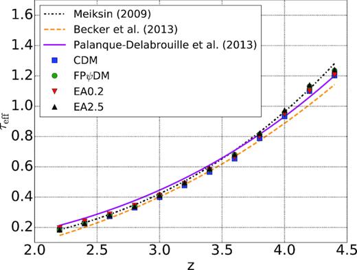
The best-fitting τeff’s of CDM, FPψDM, EA0.2, and EA2.5 simulations at each redshift bin. Lines are three different empirical power laws of τeff (Meiksin 2009; Becker et al. 2013; Palanque-Delabrouille et al. 2013). Note that the best-fitting τeff of all dark matter models are similar and consistent with the lines.
3 RESULTS
3.1 Matter power spectrum
We first present the 3D matter power spectrum of dark matter in co-moving coordinate at z = 2.2, 3.0, and 4.4 with identical cosmological parameters and m22 = 1.1. Fig. 5 shows the non-linear 3D matter power spectra of four different dark matter models from (25 h−1 Mpcc, 2 × 5123) simulations and (100 h−1 Mpcc, 2 × 5123) simulations. They are indistinguishable at low-k and diverging at high-k. The 3D matter power spectra of all EAψDM are always larger than those of FPψDM at high-k, and the result shows that the small-scale suppression in the initial matter power spectra of EAψDM has been erased to various degrees, and they are replaced by non-linear cascade spectra from the spectral bumps on the intermediate scale after evolution.
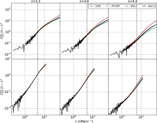
3D matter power spectra of different dark matter models at z = 2.2, 3.0, and 4.4. The difference in high-k among four simulations reveals the effects of simulation resolution and non-linearity on the shape of transfer functions. The dashed lines mark the Nyquist k of the BOSS data kNy, BOSS. Upper panels: results from (25 h−1 Mpcc, 2 × 5123) simulations. Lower panels: results from (100 h−1 Mpcc, 2 × 5123) simulations.
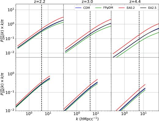
Similar to Fig. 5, here shows 1D matter power spectra of different dark matter models at z = 2.2, 3.0, and 4.4, mimicking the flux power spectra. The dashed lines mark the Nyquist k of the BOSS data kNy, BOSS. Upper panels: results from (25 h−1 Mpcc, 2 × 5123) simulations. Lower panels: results from (100 h−1 Mpcc, 2 × 5123) simulations.
3.2 Comparison simulated Lyman-α flux power spectrum with BOSS data
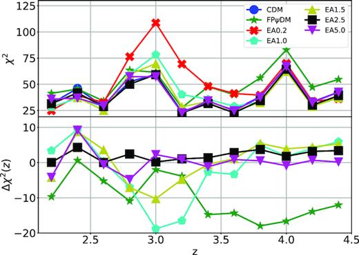
Upper panel: The χ2 distributions of different simulations at each redshift bin. Two abnormal peaks occur at redshift bins |$z$| = 3 and |$z$| = 4 for all models, while other redshift bins appear distributed normally. Lower panel: The difference of the χ2 distributions of various dark matter models from the χ2 distributions of CDM through |$\Delta \chi ^{2}(z) = \chi ^{2}_{\rm CDM}(z) - \chi ^{2}_{\rm other}(z)$|.
Best-fitting |$\chi ^2_{\rm total}$|’s of all models.
| Name of model | |$\chi ^2_{\rm total}$| |
|---|---|
| CDM | 481.1 |
| EAψDM (δθ = 0.2°) | 619.6 |
| EAψDM (δθ = 1.0°) | 499.6 |
| EAψDM (δθ = 1.5°) | 475.3 |
| EAψDM (δθ = 2.5°) | 456.8 |
| EAψDM (δθ = 5.0°) | 478.3 |
| FPψDM | 601.9 |
| Name of model | |$\chi ^2_{\rm total}$| |
|---|---|
| CDM | 481.1 |
| EAψDM (δθ = 0.2°) | 619.6 |
| EAψDM (δθ = 1.0°) | 499.6 |
| EAψDM (δθ = 1.5°) | 475.3 |
| EAψDM (δθ = 2.5°) | 456.8 |
| EAψDM (δθ = 5.0°) | 478.3 |
| FPψDM | 601.9 |
Actually, in this work we have not thoroughly optimized the assumed best model, EA2.5, having a fixed mb (to 1.1 × 10⁻²² eV) and only coarsely sampling δθ. In addition, the cosmological parameters should have also been optimized for all EAψDM simulations, but we instead fix these parameters to the one value optimized for the CDM model in favour of CDM. These two factors will affect the above evaluation of CI, but the result is unlikely to change much; moreover, these factors will also change the best values of the two degrees of freedom. If we set mb ∼ 10−22 eV as a prior given by the best fit of ψDM to the Fornax dwarf galaxy data (Schive et al. 2014a), the best EAψDM model can be estimated by interpolation of Table 1, and the best δθ lies between 2o and 4o.
4 DISCUSSIONS
We plot in Fig. 7 the χ2 distributions over the redshift range and the difference of χ2 for the CDM model from relevant EAψDM models so as to reveal detailed differences. With the latter, one clearly observes that EA2.5 has similar but slightly smaller χ2 than CDM at all redshifts, a reflection of the close similarity at all redshifts in matter power spectra of the two models as shown in Figs 5 and 6. We also find that EA5.0 has similar χ2 as CDM except at low redshifts.
We however find two distinct peaks in χ2 distributions for all dark matter models at the same redshifts. This unusual behaviour suggests that the predicted 1D flux power spectra have non-negligible systematic deviations from the BOSS data near |$z$| = 3.0 and |$z$| = 4.0 that calls for attention. On the other hand, Δχ2 shows no such distinct features, indicating that this problem is likely related to gas physics and not cosmological models.
The fact that χ2(|$z$|) gets abruptly enhanced at |$z$| = 4 may have been related to the problem of the BOSS data quality. Fig. 8 compares the flux power spectra data of BOSS (Palanque-Delabrouille et al. 2013) and XQ-100 (Iršič et al. 2017c) at |$z$| = 4.0, clearly revealing that the BOSS spectrum is inconsistent with XQ-100 spectrum at high-k bins. Our best-fitting spectra tend to follow the XQ-100 spectrum more closely than the BOSS spectrum at high-k. We have also checked the consistency between the BOSS data and the XQ-100 data in other redshift bins and found that, except for |$z$| = 4.0, they are all consistent. Therefore, this peak of χ2(|$z$|) at |$z$| = 4 is likely caused by some systematic errors of high-k BOSS data at this redshift.
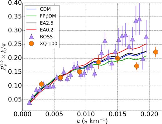
The transmitted flux power spectra of BOSS (Palanque-Delabrouille et al. 2013), XQ-100 (Iršič et al. 2017c), and model predictions at |$z$| = 4.0. It clearly shows that the power of BOSS is higher than that of XQ-100 around k > 0.015 s km−1, while the predictions are closer to the latter than to the former.
The absence of non-uniform ionization of helium gas in our simulations may explain the poor match of our predictions with the data at |$z$| = 3. Recent observations suggest that the helium reionization epoch had been started at |$z$| ≳ 3.0 and ended at |$z$| ≃ 2.7: (a) a helium Gunn-Peterson trough at |$z$| ≃ 3.0 was reported by Syphers & Shull (2014), indicating that reionization of helium is not completed by that time, but (b) HeIII Lyα has already become transparent at |$z$| ≃ 2.7 (Worseck et al. 2011). It has been asserted that despite the presence of local UV sources, uniform UVB can be a good approximation for |$z$| ∼ 2–4, except |$z$| = 2.7–3, due to large UV mean free paths. But during |$z$| ∼ 2.7–3.0, intense UV radiation from the onset of quasars renders the helium rapidly reionized. Helium reionization reduces the UV mean free path and is patchy, thus yielding local UV heating (La Plante et al. 2017). Our simulations assume uniform UVB and do not take the non-uniform UV heating into account. This problem possibly leads to the more substantial deviation of our predictions from the BOSS data around |$z$| = 3 than expected.
5 CONCLUSION
In this paper, we investigate the viability of EAψDM to explain Lyα forest absorption spectra. Our N-body hydrodynamical simulations in the wave-like dark matter scenario are based on three hypotheses. (I) Quantum effects are approximately represented by modification on the linear matter power spectrum. (II) UV background is spatially uniform and gas is optically thin and in ionization equilibrium. (III) The cosmological parameters are the same as the one optimized for the CDM model. Our simulations produce predicted Lyα absorption spectra from different dark matter scenarios upon applying a posterior process discussed in Section 2.4. Confronting the low-resolution BOSS data, we have approximately identified that the EAψDM model with δθ ∼ 2.5 best matches the observation assuming mb = 1.1 × 10⁻²² eV. The more precise value of δθ likely lies in the range of 2.0o−4.0o through interpolation from Table 1.
Our results further show that the predicted Lyα flux power spectra in the CDM model produce a significantly larger |$\chi ^2_{\rm total}(= 481)$| than the best EAψDM model of (mb, δθ) = (1.1 × 10⁻²² eV, 2.5o) does with |$\chi ^2_{\rm total} = 456.8$|. Though all cosmological parameters used in EAψDM simulations are optimized for CDM, the best EAψDM model still provides the smallest |$\chi ^2_{\rm total}$|. The difference between the best EAψDM model and the CDM model is statistically significant and the CDM model is outside the confidence interval CI ∼ 1–10−5, assuming that EA2.5 is the best model.
High-resolution data, such as XQ-100 and HIRES/MIKE, can provide stronger constraints on the axion mass and the axion angle. (See the demonstration in Appendix C.) However, as discussed in Section 3.1, quantum effects become important at low redshift for mb ∼ 10−22 eV when the spectral resolution becomes as high as these data. These wave interference effects are beyond the capability of the N-body hydro simulation presently employed and can be reliably captured in wave simulations or possibly captured in hydro simulations with approximate modelling of quantum pressure (Li et al. 2018; Nori & Baldi 2018; Nori et al. 2019), which await further investigations. In addition, the stellar/AGN feedback discussed below may no longer be neglected again at low redshift due to metal cooling (Viel et al. 2013) in simulations that are to address the high-resolution data.
Most Lyα simulation works do not take into account mechanical feedback from stars, which is clearly an important source for local IGM turbulence and heating. This issue may cause concerns for the credibility of the predicted flux spectrum. Here we present an argument in favour of the BOSS data. The BOSS data have the highest spatial resolution about kNy ∼ 5 h Mpcc−1 or a physical wavelength 200 kpc around |$z$| ∼ 3, and hence stellar mechanical feedback is unlikely to reach this large scale. Only AGN mechanical feedback may possibly impact on high-k spectra of BOSS. But AGNs are rare and moreover their activities peak at |$z$| = 2, which is after the lowest redshift of the BOSS data at |$z$| = 2.2. Therefore the BOSS data should be free from contamination of the stellar feedback and may be free from contamination of the AGN feedback.
We have assumed in this work a uniform UV background that gives rise to global heating. But local UV heating can also be significant, especially around |$z$| = 2.7–3, and such local UV heating has not been included in our simulations. Unlike local stellar feedback, local UV sources from quasars, which reionize helium thereby heating the gas near |$z$| = 3, can have an impact on scales spanned by the BOSS data. Despite the fact that UV sources are non-trivial to model, some simple heating recipe may indeed bring the predicted flux spectrum in closer agreement with the BOSS data. As demonstrated in (Armengaud et al. 2017), incorporating empirical local UV heating yields |$\chi ^2_{\rm total,CDM} = 405$| rather than |$\chi ^2_{\rm total,CDM} = 481$| in our prediction. Although some fitting parameters in that work are different from ours, which may affect |$\chi ^2_{\rm total}$|, the χ2 peak around |$z$| = 3 in Fig. 7 has a major contribution to the increase of |$\chi ^2_{\rm total,CDM}$| in our prediction. This aspect needs improvements in the future work. We also notice that both the CDM model and the EA2.5 model have almost identical large χ2’s at |$z$| = 2.8 and |$z$| = 3 bins in Fig. 7. Affected only by the gas physics rather than underlying dark matter models, in a work with proper local heating to bring down χ2’s of these two bins, the revised values of χ2’s in both models are likely comparable. Hence, the difference of |$\chi ^2_{\rm total}$|’s in these two models would not be much affected.
Recent studies on the predicted Lyα flux spectra of free-particle (FP) ψDM placed a lower bound for the particle mass, mb ≳ 2.9 × 10⁻²¹ eV (Armengaud et al. 2017) and mb ≳ 3.75 × 10⁻²¹ eV (Iršič et al. 2017b) (see also Nori & Baldi 2018), which are in tension with the particle mass determined from local satellite galaxies (Schive et al. 2014a; Chen et al. 2017), mb ∼ 1 × 10⁻²²–3 × 10⁻²² eV. This work demonstrates that such tension can be removed when the extreme axion misaligned angle is taken into account, i.e. EAψDM models, even for the lowest particle mass mb ∼ 10−22 eV determined from local galaxy data (Schive et al. 2014a). Due to the lack of local UV heating and various physical effects not taken in account in this demonstrative work, we do not obtain a |$\chi ^2_{\rm total}$|’s as small as they should have been and cannot ascertain the exact values of optimal axion angle δθ and particle mass mb. Moreover, the simple global UV heating model of Haardt & Madau (2012), which we have adopted, may have slight rooms to optimize (cf. Fig. 2) through varying the global heating rate to further constrain the best model. Despite all these, the tendency of a possible superior extreme axion wave dark matter model over, or a comparable model to, the CDM model against the BOSS Lyα forest data is already evident.
Finally, we would like to put the finding of the best initial axion angle θ0 into a perspective of the axion model. In the axion model, f, the decay constant, also characterizes the axion symmetry-breaking energy scale, and f is on one hand determined by matching the matter energy density |$m_\mathrm{ b}^2 c^2 f^2 \theta ^2$| equal to the radiation energy density at the radiation-matter equality. Well prior to the equality, θ2 is decreasing with the scaling factor as (a/aeq)−3, where aeq is the scaling factor at the equality, and the matter energy density behaves as CDM does. But this a−3 scaling occurs only after the Zitterbewegun oscillation starts at aosc; before the oscillation the matter energy density is a constant. As a result, the matter energy density at the very early epoch on the other hand is |$m_\mathrm{ b}^2c^2 f^2\theta _0^2 \sim \epsilon _{\mathrm{ rad, eq}} (a_{\mathrm{ eq}}/a_{\mathrm{ osc}})^3$|, where εrad, eq is the radiation energy density at the equality. The squared decay constant |$f^2 = \epsilon _{\mathrm{ rad, eq}}(a_{\mathrm{ eq}}/a_{\mathrm{ osc}}(\theta _0))^3/m_\mathrm{ b}^2 c^2\theta _0^2$|, and this quantity turns out to be a decreasing function of θ0. For example, the FPψDM model, where θ0 → 0, has the axion symmetry-breaking scale |$f \rightarrow \theta _0^{-1}$|, and the symmetry-breaking scale may exceed the Planck scale. For mb = 1.1 × 10⁻²² eV and δθ0 = 5°, 2.5°, 1.5°, the three initial angles found to have smaller |$\chi ^2_{\rm total}$| than the CDM model, we have the symmetry-breaking scale f = 2.66 × 10¹⁶, 2.32 × 10¹⁶, and 2.13 × 10¹⁶ GeV, slightly above the typical grand unified theory energy scale 1016 GeV, which is also the fiducial energy scale of the inflation. The axion symmetry-breaking energy scale above or equal to the inflation energy scale has an important merit that topological defects, such as domain walls arising from different parts of the universe having different values of θ0’s can be inflated away, therefore ensuring that we have one and only one value of θ0 in the visible universe, as assumed in this work. Interestingly, if we let mb to vary and mb > 10−22 eV, all axion symmetry-breaking scale should exceed the fiducial inflation scale. This is because |$a_{\rm osc}\propto m_\mathrm{ b}^{-1/2}g(\theta _0)$| for some function g of θ0, we find f only weakly depends on mb as |$\propto m_\mathrm{ b}^{-1/4}g^{3/2}(\theta _0)\theta _0^{-1}$|, and both g(θ0) and |$\theta _0^{-1}$| are increasing functions of mb when the optimal θ0 for the Lyα data is taken into account, which compensate the weak dependence of |$m_\mathbf{ b}^{-1/4}$|.
ACKNOWLEDGEMENTS
We thank Dr. Phil Hopkins making the GIZMO code available to us. T.C. acknowledges the funding support from MOST of Taiwan under the grant, MOST 107-2119-M-002-036-MY3. This publication is supported in part by the Jade Mountain Young Scholar Award (No. 107V0201) to H.S.
Footnotes
REFERENCES
APPENDIX A: SPLICING METHOD
In Section 2.3, we mentioned that we simulated |$P^{\rm 1D}_{\rm F}$| through the splicing method (McDonald 2003; Borde et al. 2014) to reduce the computation time for hydrodynamical simulations. In practice, different simulations with varying resolutions and with varying box sizes provide different dynamical ranges of k. In this appendix, we present our tests of the splicing method.
We then construct the composite flux power spectrum with (L, N) = (100 h−1 Mpcc, 2 × 5123) obtained by merging the three flux spectra of (L, N) = (25 h−1 Mpcc, 2 × 323), (L, N) = (25 h−1 Mpcc, 2 × 1283), and (L, N) = (100 h−1 Mpcc, 2 × 1283), and compare the composite flux spectrum with the exact flux power spectra of (L, N) = (100 h−1 Mpcc, 2 × 5123). In Fig. A1, we illustrate the goodness of splicing at |$z$| = 3.0 for the CDM model. The error of splicing method is at most |$8{{\ \rm per\ cent}}$| at every redshift over the entire k-range of interest. The errors in other redshifts are comparable to this characteristic value.
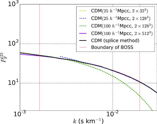
Test of the splicing method for the CDM model. The pink line is the exact transmitted flux power spectra from (100 h−1 Mpcc, 2 × 5123) simulation and the red line is the spliced transmitted flux power spectra composite flux power spectra from (100 h−1 Mpcc, 2 × 1283), (25 h−1 Mpcc, 2 × 1283), and (25 h−1 Mpcc, 2 × 323) simulations. The vertical lines are the range of the BOSS data in use.
APPENDIX B: NUMERICAL CONVERGENCE
As our ψDM model simulations are based on the CDM-hydro simulation with modified initial matter power spectra (see Section 2.2), the convergence test for the CDM simulation alone should adequately reflect the convergence behaviours of the simulated flux power spectra of all dark matter models. We choose |$P_{\rm F,25, 512}^{\rm 1D}(k)$| as the reference spectrum and define |$(\pm \sigma _{\rm BOSS}(k) / P_{\rm F,25, 512}^{\rm 1D}(k)) + 1$| as the normalized data uncertainty, where σBOSS is the 1 − σ uncertainties of the BOSS data. We show the convergence test at |$z$| = 3.0 in Fig. B1, where the relative flux power spectra of (25 h−1 Mpcc, 2 × 1283) and (25 h−1 Mpcc, 2 × 2563) simulations are shown along with the normalized data uncertainty. It is clear that the (25 h−1 Mpcc, 2 × 2563) flux power spectrum is within 1σBOSS and converges to within ∼5 per cent of the reference spectrum. Linearly extrapolating |$P_{\rm F,\rm sim}^{\rm 1D}(k) / P_{\rm F,\rm ref}^{\rm 1D}(k) - 1$| in log-space, it follows that the difference between the flux power spectra of (25 h−1 Mpcc, 2 × 5123) and (25 h−1 Mpcc, 2 × 10243) simulations is within 0.2σBOSS. This amount of simulation errors may somewhat enhance the total χ2 listed in Table 1, but a quantitative estimate of the enhancement is non-trivial to assess.
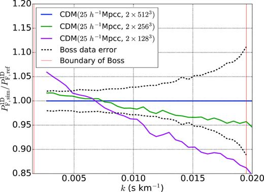
Convergence test in the CDM at |$z$| = 3.0, where we choose the transmitted flux power spectrum of the (25 h−1 Mpcc, 2 × 5123) simulation as the reference. The blue line, the green line, and the pink line are the transmitted flux power spectra from (25 h−1 Mpcc, 2 × 5123), (25 h−1Mpcc, 2 × 2563), and (25 h−1Mpcc, 2 × 1283) simulations, respectively. The black dash line represents the normalized 1σ uncertainties measured in the BOSS data and the vertical red lines are the range of the BOSS data in use.
APPENDIX C: SAMPLE LYα ABSORPTION SPECTRA
We here show a set of sample-simulated spectra (|$z$| = 2.2, 3.2, and 4.4) of different models along the same line of sight in Fig. C1, with which Fourier transform is performed to obtain flux power spectra and the average power spectrum over 105 samples is to be compared with the BOSS data. From individual Lyα spectra at |$z$| = 2.2 and 3.2, it is difficult to detect any systematic difference among different models, partly because the lack of neutral hydrogen at these redshifts renders the absorption feature less prominent and partly because different models have already been highly evolved, which erases the feature of the initial matter power spectrum. By contrast at |$z$| = 4.4, the substantially more abundant neutral hydrogen makes the absorption feature more distinct and the dark matter is less evolved than low redshifts. We can clearly see that the CDM model has large variations in the absorption spectrum than the two ψDM models, where low absorption regions tend to have lower absorption and high absorption regions tend to have higher absorption, indicative of a more clumpy universe for the CDM model. It also demonstrates that high-|$z$| Lyα forest data are crucial for probing the difference in initial power spectra of different models.
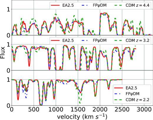
Simulated spectra for EA2.5, FPψDM, and CDM at |$z$| = 4.4, 3.2, 2.2.
APPENDIX D: BEST-FITTED TRANSMITTED FLUX POWER SPECTRA
We show in detail best-fitted flux power spectra of various dark matter models compared with the BOSS spectrum as shown in the 13 figures in this Appendix. All predicted flux power spectra are almost identical for |$z$| < 2.6. The predicted flux power spectra begin to diverge when |$z$| > 3. In particular, the difference among all predicted flux power spectra is significant for |$z$| > 3.8. This suggests that the structure evolution is diverging at high redshift but become similar at the low redshift, which is supported by the evolution of matter power spectra of different dark matter models (Fig. 5). However, the model difference is offset by the ever-increasing observational data errors with increasing redshifts making it difficult to tell better models without summing up k-bins as being done in Fig. 7.
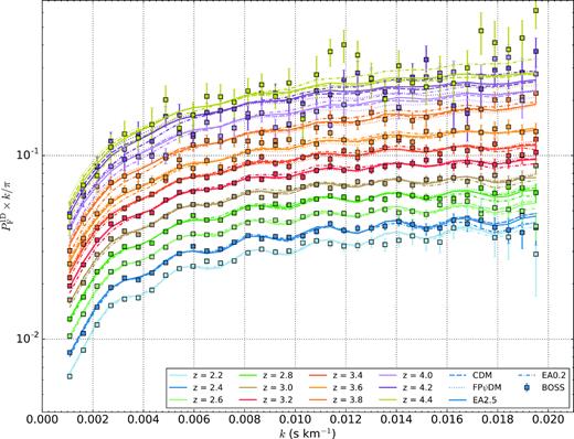
Best-fitted transmitted flux power spectra of CDM, FPψDM, EA0.2, and EA2.5 and the BOSS data (Palanque-Delabrouille et al. 2013) at each redshift bin.
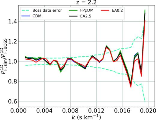
Best-fitted results at |$z$| = 2.2.
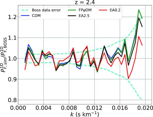
Best-fitted results at |$z$| = 2.4.
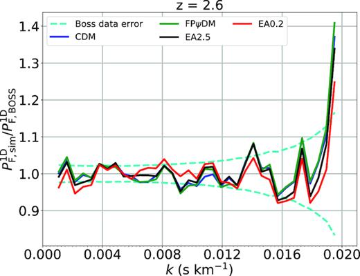
Best-fitted results at |$z$| = 2.6.
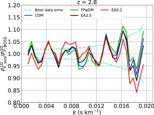
Best-fitted results at |$z$| = 2.8.
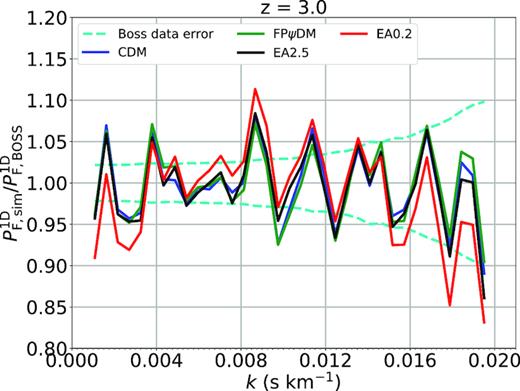
Best-fitted results at |$z$| = 3.0.
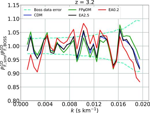
Best-fitted results at |$z$| = 3.2.
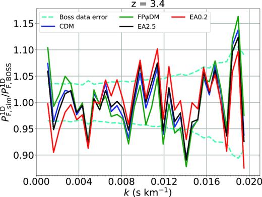
Best-fitted results at |$z$| = 3.4.
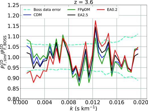
Best-fitted results at |$z$| = 3.6.
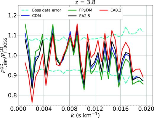
Best-fitted results at |$z$| = 3.8.
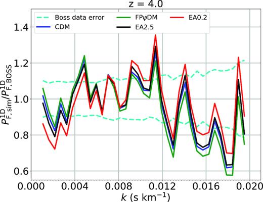
Best-fitted results at |$z$| = 4.0.
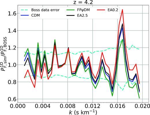
Best-fitted results at |$z$| = 4.2.
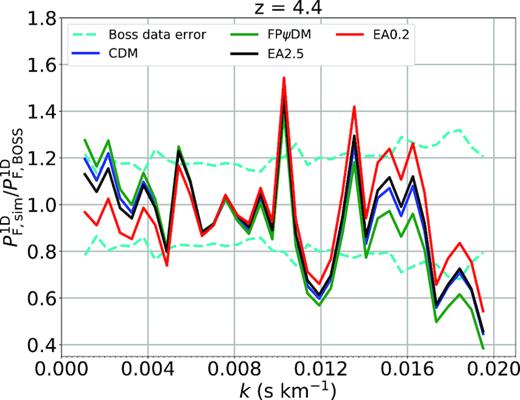
Best-fitted results at |$z$| = 4.4.
