


ABSTRACT
We present new synthesis models of the extragalactic background light (EBL) from far infra-red (FIR) to TeV γ-rays, with an emphasis on the extreme ultraviolet (UV) background that is responsible for the observed ionization and thermal state of the intergalactic medium across the cosmic time. Our models use updated values of the star formation rate density and dust attenuation in galaxies, QSO emissivity, and the distribution of H|$\, \, {\rm {\scriptstyle I}}$| gas in the intergalactic medium. Two of the most uncertain parameters in these models, the escape fraction of H|$\, \, {\rm {\scriptstyle I}}$| ionizing photons from galaxies and the spectral energy distribution (SED) of QSOs, are determined to be consistent with the latest measurements of H|$\, \, {\rm {\scriptstyle I}}$| and He|$\, \, {\rm {\scriptstyle II}}$| photoionization rates, the He|$\, \, {\rm {\scriptstyle II}}$| Lyman-α effective optical depths, various constraints on H|$\, \, {\rm {\scriptstyle I}}$| and He|$\, \, {\rm {\scriptstyle II}}$| reionization history, and many measurements of the local EBL from soft X-rays till γ-rays. We calculate the EBL from FIR to TeV γ-rays by using FIR emissivities from our previous work and constructing an average SED of high-energy emitting QSOs, i.e, type-2 QSOs and blazars. For public use, we also provide the EBL models obtained using different QSO SEDs at extreme-UV energies over a wide range of redshifts. These can be used to quantify uncertainties in the parameters derived from photoionization models and numerical simulations originating from the allowed variations in the UV background radiation.
1 INTRODUCTION
The radiation background set-up by light emitted from all galaxies and Quasi-Stellar Objects (QSOs) throughout the cosmic time is known as extragalactic background light (EBL). The full spectrum of EBL carries imprints of cosmic structure formation; therefore, it serves as an important tool to study formation and evolution of galaxies. It is also essential for studying the propagation of high energy γ-rays from distant sources since the EBL can annihilate γ-rays upon collision (Gould & Schréder 1966; Stecker, de Jager & Salamon 1992; Ackermann et al. 2012). The EBL is playing a key role in rapidly developing γ-ray astronomy to address fundamental questions related to the production of γ-rays, their acceleration mechanism (Stecker, Baring & Summerlin 2007), and cosmic magnetic fields in the intergalactic space (Neronov & Vovk 2010; Tavecchio et al. 2011; Arlen et al. 2014; Finke et al. 2015).
A small part of this EBL at extreme-UV energies (E > 13.6 eV or λ < 912 Å) is known as the UV background (UVB). The UVB is responsible for maintaining the observed ionization and thermal state of the diffuse intergalactic medium (IGM; see reviews by Meiksin 2009; McQuinn 2016), a reservoir that is believed to contain more than 90 per cent of total baryons in the Universe.
The sources that set up the UVB also drive the major phase transitions of the IGM, the H|$\, \, {\rm {\scriptstyle I}}$|, and He|$\, \, {\rm {\scriptstyle II}}$| reionization. Starting from the time when first galaxies were born, the process of H|$\, \, {\rm {\scriptstyle I}}$| reionization is believed to be completed around |$z$| ∼ 6 as suggested by various observations of H|$\, \, {\rm {\scriptstyle I}}$| Lyman-α forest in the spectra of high redshift QSOs (e.g. Becker et al. 2001; Fan et al. 2006; Goto et al. 2011; McGreer, Mesinger & D’Odorico 2015; Bañados et al. 2018; Greig et al. 2017; Davies et al. 2018), electron scattering optical depth to the cosmic microwave background (CMB; Larson et al. 2011; Planck Collaboration XIII 2016a) and decreasing fraction of Lyman-α emitting galaxies at high redshifts (e.g. Schenker et al. 2014; Choudhury et al. 2015; Mesinger et al. 2015; Mason et al. 2018). The He|$\, \, {\rm {\scriptstyle II}}$| reionization is believed to be started by hard He|$\, \, {\rm {\scriptstyle II}}$| ionizing radiation emitted by QSOs and took longer time to complete. It was completed around |$z$| ∼ 2.8 as suggested by observations of He|$\, \, {\rm {\scriptstyle II}}$| Lyman-α forest in a handful of QSOs (e.g. Kriss et al. 2001; Shull et al. 2004, 2010; Fechner et al. 2006; Worseck et al. 2011, 2016) and measurements of a peak in the redshift evolution of IGM temperature (Lidz et al. 2010; Becker et al. 2011; Hiss et al. 2018; Walther et al. 2018). During these reionization events, spectrum of the UVB decides the extra energy gained by photoelectrons, which gets redistributed in the IGM driving its thermal state (Hui & Gnedin 1997). Subsequently the thermal history of the IGM is driven by the UVB and adiabatic expansion of the Universe.
Thermal history of the IGM has its imprint on the small-scale structures in the IGM through pressure smoothing that can be probed by correlation analysis of closely spaced QSO sightlines (e.g. Gnedin & Hui 1998; Schaye 2001; Kulkarni et al. 2015; Rorai et al. 2017). Photoheating by the UVB can also provide negative feedback that can suppress the star formation in dwarf galaxies (Efstathiou 1992; Weinberg, Hernquist & Katz 1997) and decide the faint end shapes of the high-z luminosity functions (e.g. Samui, Srianand & Subramanian 2007). Therefore the UVB is one of the most important inputs in the cosmological simulations of structure formation and the IGM (e.g, Hernquist et al. 1996; Davé et al. 1999; Springel, Yoshida & White 2001).
Perhaps the most important and frequent application of UVB is to study the metal absorption lines ubiquitously observed in QSO absorption spectra. It is because the EBL from extreme-UV to soft X-ray ionizes not only hydrogen and helium but also several metals such as Mg, C, Si, N, O, and Ne. Therefore, the UVB serves as an essential ingredient to study the physical and chemical properties of the gas observed in the QSO absorption spectra originating either from low-density gas in the IGM or from high-density gas in the vicinity of intervening galaxies known as a circumgalactic medium (CGM). In the studies of metal absorption lines, the UVB is crucial for relating observed ionic abundances to metal abundances, in order to determine the metal production and their transport to CGM by galaxies (e.g. Ferrara, Scannapieco & Bergeron 2005; Lehner et al. 2014; Peeples et al. 2014) and the time evolution of the cosmic metal density (e.g. Songaila & Cowie 1996; Bergeron et al. 2002; Schaye et al. 2003; Aracil et al. 2004; D’Odorico et al. 2013; Shull, Danforth & Tilton 2014; Muzahid et al. 2018; Prochaska et al. 2017). At low redshifts, the UVB is essential for studying the ionization mechanism of highly ionized species such as O vi (e.g. Danforth & Shull 2005; Tripp et al. 2008; Muzahid et al. 2012; Savage et al. 2014; Pachat et al. 2016; Narayanan et al. 2018) and Ne viii (e.g. Savage et al. 2005, 2011; Narayanan, Savage & Wakker 2012; Meiring et al. 2013; Hussain et al. 2015, 2017; Pachat et al. 2017) to understand their contribution to the warm-hot IGM and missing baryons (see Shull et al. 2012).
The local EBL (|$z$| = 0) at most wavelength ranges can be observed directly (e.g. Dwek & Arendt 1998; Dole et al. 2006; Ajello et al. 2008); however, there are no such direct observations of the UVB because the interstellar medium of our Milky way attenuates it completely. Therefore, one needs to model the UVB spectrum and its redshift evolution. There are, however, integral constraints on the UVB obtained from the measurements of H|$\, \, {\rm {\scriptstyle I}}$| and He|$\, \, {\rm {\scriptstyle II}}$| photoionization rates. The H|$\, \, {\rm {\scriptstyle I}}$| photoionization rates (|$\Gamma _{\rm H \, {\scriptscriptstyle I}}$|) can be measured by using the observations of 21 cm truncation and Hα fluorescence in nearby galaxies (e.g. Sunyaev 1969; Dove & Shull 1994; Adams et al. 2011; Fumagalli et al. 2017), by analyzing the incidence of Lyman-α forest lines in the proximity of QSOs (e.g. Bajtlik, Duncan & Ostriker 1988; Kulkarni & Fall 1993; Srianand & Khare 1996; Dall’Aglio, Wisotzki & Worseck 2008), and by reproducing various statistical properties of the observed Lyman-α forest in the cosmological simulations of the IGM where |$\Gamma _{\rm H \, {\scriptscriptstyle I}}$| is treated as one of the free parameters (e.g. Rauch et al. 1997; Bolton & Haehnelt 2007; Becker & Bolton 2013; Kollmeier et al. 2014; Shull et al. 2015; Gaikwad et al. 2017a,b, 2018b). One can also infer the He|$\, \, {\rm {\scriptstyle II}}$| photoionization rate (|$\Gamma _{\rm He \, {\scriptscriptstyle II}}$|) using the measurements of |$\Gamma _{\rm H \, {\scriptscriptstyle I}}$| and the observed H|$\, \, {\rm {\scriptstyle I}}$| column density distribution as demonstrated in Khaire (2017). These measurements play a crucial role in calibrating the synthesis models of UVB at different redshifts.
The full synthesis model of UVB was pioneered by Haardt & Madau (1996) (see also Fardal, Giroux & Shull 1998) using cosmological radiative transfer calculations following the footsteps of the previous work (Miralda-Escude & Ostriker 1990; Shapiro, Giroux & Babul 1994; Giroux & Shapiro 1996). Over the last two decades, there are some variations of their UVB models (Haardt & Madau 2001, 2012) and the UVB models by other groups (Shull et al. 1999; Faucher-Giguère et al. 2009). Out of these, most recent models1 are Faucher-Giguère et al. (2009, hereafter FG09) and Haardt & Madau (2012, hereafter HM12). These recent models are not completely consistent with the new observations such as |$\Gamma _{\rm H \, {\scriptscriptstyle I}}$| at |$z$| < 0.5 (Shull et al. 2015; Gaikwad et al. 2017a,b; Gurvich, Burkhart & Bird 2017; Viel et al. 2017) and |$z$| > 3 (Becker & Bolton 2013). These models also use old values of many observables relevant to UVB that are significantly different from current measurements, such as the type 1 QSO emissivity (Khaire & Srianand 2015a, hereafter KS15a), galaxy emissivity (Behroozi, Wechsler & Conroy 2013; Madau & Dickinson 2014; Khaire & Srianand 2015b, hereafter KS15b); and various constraints on H|$\, \, {\rm {\scriptstyle I}}$| and He|$\, \, {\rm {\scriptstyle II}}$| reionization (Choudhury et al. 2015; Planck Collaboration XLVI 2016b; Worseck et al. 2016; Greig & Mesinger 2017). In light of all these issues, and the fact that there are only few independent UVB models available in the literature, we present new synthesis models of EBL focusing on the UVB and extending it till TeV γ-rays from far infra-red (FIR).
In our EBL models we use the updated type 1 QSO emissivity obtained from a compilation of recent QSO luminosity functions (QLFs) KS15a. Our models use galaxy emissivity till FIR wavelengths obtained from the updated star formation and dust attenuation history of the Universe from KS15b. These are determined through a large compilation of multiwavelength galaxy luminosity functions (GLFs; see KS15b, and references therein). We also use updated H|$\, \, {\rm {\scriptstyle I}}$| distribution of the IGM from Inoue et al. (2014) that is obtained from a large number of different observations (mentioned in Section 2). Apart from these, there are two additional important input parameters required to model the UVB; the average escape fraction of H|$\, \, {\rm {\scriptstyle I}}$| ionizing photons from galaxies (fesc) and the mean spectral energy distribution (SED) of type 1 QSOs at extreme-UV wavelengths. However, the observational constraints on these are either not available or poor.
The measurement of fesc from individual galaxies as well as large surveys has been proven to be a challenging endeavour (Vanzella et al. 2010; Mostardi et al. 2015; Siana et al. 2015). There are a handful of galaxies at |$z$| < 0.5, which show emission of H|$\, \, {\rm {\scriptstyle I}}$| ionizing photons with fesc ranging from 2 to 46 per cent (Bergvall et al. 2006; Leitet et al. 2013; Borthakur et al. 2014; Izotov et al. 2016b,a, 2018; Leitherer et al. 2016; Puschnig et al. 2017) and only two galaxies at |$z$| > 3 with large fesc of the order of 50 per cent (de Barros et al. 2016; Shapley et al. 2016; Vanzella et al. 2016). However, all of these are few exceptional cases, as most studies with a large number of galaxies provide only upper limits on the average fesc (e.g. Cowie, Barger & Trouille 2009; Bridge et al. 2010; Siana et al. 2010; Guaita et al. 2016; Smith et al. 2016; Grazian et al. 2017; Japelj et al. 2017; Matthee et al. 2017; see left-hand panel of Fig. 3 and Table A1 for a summary of recent measurements). On the other hand, there are measurements of QSO SED at extreme-UV from a large number of QSOs probing rest-wavelength λ < 912 Å (e.g, Zheng et al. 1997; Telfer et al. 2002; Scott et al. 2004; Shull et al. 2012; Stevans et al. 2014; Lusso et al. 2015; Tilton et al. 2016). However, under the assumption that QSO SED follows a power law, fν ∝ να at λ < 912 Å , the values of power-law index α obtained from these measurements show large variation (−0.56 to −1.96; see table 1 of Khaire 2017, for the summary of these measurements). Also, the smallest wavelength probed in these studies is ∼425 Å whereas the UVB model calculations extrapolate it upto soft X-rays (λ ≲ 20 Å).
Because of these uncertainties, we choose to determine fesc(|$z$|) and α, which are required to consistently reproduce various observational constraints on the UVB following Khaire et al. (2016) and Khaire (2017). We obtain the fesc(|$z$|) to reproduce the |$\Gamma _{\rm H \, {\scriptscriptstyle I}}$| measurements and various constraints on H|$\, \, {\rm {\scriptstyle I}}$| reionization. In our fiducial UVB model, we use α = −1.8, which was found to reproduce the measured He|$\, \, {\rm {\scriptstyle II}}$| Lyman-α effective optical depths as a function of |$z$| and the epoch of He|$\, \, {\rm {\scriptstyle II}}$| reionization (see Khaire 2017). However, we also provide UVB models for α varying from −1.4 to −2.0 in the interval of 0.1. Moreover, following Sazonov, Ostriker & Sunyaev (2004), we modify the SED of type 1 QSOs to include the type 2 QSOs and blazars in order to calculate the X-ray and γ-ray part of the EBL consistent with various measurements of the local X-ray and γ-ray backgrounds. Our full EBL spans more than 15 orders of magnitude in wavelength from FIR to TeV γ-rays.
The paper is organized as follows. In Section 2, we briefly discuss the basic cosmological radiative transport theory used for calculating the EBL. In Section 3, we explain the emissivities used in our EBL. We discuss the QSO emissivity, their SEDs, the galaxy emissivity, fesc(|$z$|), and the diffuse emissivity from the IGM. In Section 4, we discuss our fiducial model and its predictions for H|$\, \, {\rm {\scriptstyle I}}$| and He|$\, \, {\rm {\scriptstyle II}}$| photoionization rates, reionization histories, full spectrum of the EBL from FIR to γ-rays, and the detailed uncertainties in the UVB models. In Section 5, we summarize our main results. In the Appendix we show plots for various UVB models generated for different α and provide relevant tables of photoionization and photoheating rates and optical depths encountered by γ-ray photons due to the EBL. Throughout the paper, we have used the cosmological parameters Ωm = 0.3, ΩΛ = 0.7 and H0 = 70 km s−1 Mpc−1 consistent with measurements from Planck Collaboration XIII (2016a). All our EBL tables in machine-readable format are publicly available to download (at http://www.iucaa.in/projects/cobra/ cobra-webpage & a http://vikramkhaire.weebly.com/downloads.html homepage) and latest version of cloudy software (last described in Ferland et al. 2017).
2 COSMOLOGICAL RADIATIVE TRANSFER
We take f(NHi, |$z$|) from Inoue et al. (2014) at all |$z$|. It has been obtained by fitting various observations over |$z$| = 0−6 such as the number distribution and column density distribution of optically thin H|$\, \, {\rm {\scriptstyle I}}$| Lyman-α absorbers (Weymann et al. 1998; Kim, Cristiani & D’Odorico 2001; Janknecht et al. 2006; Kim et al. 2013), optically thick Lyman limit absorbers (Péroux et al. 2005; Rao, Turnshek & Nestor 2006; Prochaska, O’Meara & Worseck 2010; Songaila & Cowie 2010; Fumagalli et al. 2013; O’Meara et al. 2013) and damped Lyman-α absorbers (O’Meara et al. 2007; Noterdaeme et al. 2009, 2012; Prochaska et al. 2014), the mean transmission and optical depth of the IGM to Lyman-α photons (Fan et al. 2006; Kirkman et al. 2007; Faucher-Giguère et al. 2008; Becker et al. 2013) and the mean free path of H|$\, \, {\rm {\scriptstyle I}}$| ionizing photons through IGM (Prochaska, Worseck & O’Meara 2009; Worseck et al. 2014). The f(NH i, |$z$|) calculated at |$z$| = 5.5 and 6 from high-resolution hydrodynamic simulations for the measured |$\Gamma _{\rm H \, {\scriptscriptstyle I}}$| values match reasonably well with the f(NHi, |$z$|) from Inoue et al. (2014), as shown in Khaire et al. (2016). This consistency motivates us to use this f(NHi, |$z$|) even at |$z$| > 6, where direct observations are not possible because of strong Gunn–Peterson effect (Gunn & Peterson 1965). See Section 4.4.3 for uncertainties in the UVB arising when different f(NHi, |$z$|) is used in our calculations.
3 EMISSIVITY
3.1 QSO Emissivity
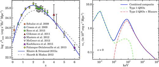
Left-hand panel: the specific QSO emissivity at 1000 Å (|$\epsilon ^Q_{\nu _{1000}}$|) with |$z$|. Data points are taken from the compilation of recent QLFs by Khaire & Srianand (2015a, see their table 1). Blue solid curve is a simple fit through the |$\epsilon ^Q_{\nu _{1000}}$| values (equation 9). Dashed curve is the |$\epsilon ^Q_{\nu _{1000}}$| used by HM12, which is obtained using the compilation of QLFs by Hopkins, Richards & Hernquist (2007). Right-hand panel: |$z$| = 0 QSO emissivity (solid curve) at different energies to illustrate our fiducial composite QSO SED (with α = −1.8; equation 11). Dashed curve and dot-dash curve show the adopted SED of Type 1 QSOs and high-energy emitting AGN template SED (i.e. Type 2 QSOs and blazars), respectively, normalized to get |$\epsilon ^Q_{\nu _{1000}}$| at |$z$| = 0.
The QSO emissivity mentioned in equation (10) is contributed by type 1 QSOs alone. Note that to calculate the background radiation in extreme-UV, one does not need to consider the contribution from type 2 QSOs. According to the standard unification scheme of active galactic nuclei (AGNs; Antonucci 1993; Urry & Padovani 1995), different classes of QSOs arise due to differences in the orientation of QSOs along the direction of obscuring torus around their central engine with respect to us. Therefore, under the assumption of isotropic distribution of randomly oriented QSOs, to calculate the extreme-UV emissivities, it is equivalent to assume that the extreme-UV photons are emitted either isotropically by type 1 QSOs alone or only along certain directions by both type 1 and type 2 QSOs. However, in the latter assumption one needs to correctly account for the fraction of type 2 QSOs. For simplicity, to calculate the UVB, we choose the former assumption. However, to extend our EBL calculation to high-energy X-rays, which are emitted isotropically by all types of QSOs, we need to incorporate contribution from type 2 QSOs.
This contribution in X-rays can be accounted self-consistently by using type 2 QLF in soft and hard X-ray band and then modeling the distribution of different hydrogen column densities in obscuring torus, using intrinsic template of X-ray SEDs of QSOs and by fixing a contribution of extremely obscured Compton thick QSOs by comparing with measurements of the unresolved X-ray background (see e.g. Comastri et al. 1995; Treister & Urry 2005; Gilli, Comastri & Hasinger 2007; Treister, Urry & Virani 2009; Ballantyne et al. 2011). Similarly the contribution to γ-ray background from blazars can be modeled by generating the blazar luminosity function and their SED from luminosity functions of radio QSOs (e.g. Draper & Ballantyne 2009).
However, these X-ray population synthesis models require different fractions of Compton thick QSOs to generate the observed peak at ∼30 keV in X-ray background and varying degree of obscuring hydrogen column densities but still may not entirely reproduce the observed soft X-ray background (see Cappelluti et al. 2017). Although this might be the most appropriate approach, given the large uncertainties involved in it, we take a more simplistic approach that can provide an observationally consistent model of the EBL in X-ray energies useful for constructing ionization models for highly ionized metal species such as O vi, O vii, Ne viii, Ne ix, and Mg x. In particular, we follow the approach of Sazonov et al. (2004) and construct a template SED of type 1 and type 2 QSOs at X-ray energies. Our type 2 QSO SED not only accounts for the contribution of Compton thick AGNs but also includes γ-rays that mostly come from beamed sources like blazars. This SED can be thought as a template SED for high-energy emitting AGNs. These SEDs are constructed such that when used in the EBL calculations they can reproduce a complete spectrum of observed X-ray and γ-ray background. The final QSO SED constructed in this way is given below.
| Model Name | α | hνa (keV) | Sk |
|---|---|---|---|
| Q14 | −1.4 | 40 | 0.4 |
| Q15 | −1.5 | 20 | 0.7 |
| Q16 | −1.6 | 8.0 | 1.0 |
| Q17 | −1.7 | 4.0 | 1.3 |
| Q18 | − 1.8 | 2.0 | 1.3 |
| Q19 | −1.9 | 1.5 | 1.6 |
| Q20 | −2.0 | 1.0 | 1.4 |
| Model Name | α | hνa (keV) | Sk |
|---|---|---|---|
| Q14 | −1.4 | 40 | 0.4 |
| Q15 | −1.5 | 20 | 0.7 |
| Q16 | −1.6 | 8.0 | 1.0 |
| Q17 | −1.7 | 4.0 | 1.3 |
| Q18 | − 1.8 | 2.0 | 1.3 |
| Q19 | −1.9 | 1.5 | 1.6 |
| Q20 | −2.0 | 1.0 | 1.4 |
Note: Q18 is our fiducial model.
| Model Name | α | hνa (keV) | Sk |
|---|---|---|---|
| Q14 | −1.4 | 40 | 0.4 |
| Q15 | −1.5 | 20 | 0.7 |
| Q16 | −1.6 | 8.0 | 1.0 |
| Q17 | −1.7 | 4.0 | 1.3 |
| Q18 | − 1.8 | 2.0 | 1.3 |
| Q19 | −1.9 | 1.5 | 1.6 |
| Q20 | −2.0 | 1.0 | 1.4 |
| Model Name | α | hνa (keV) | Sk |
|---|---|---|---|
| Q14 | −1.4 | 40 | 0.4 |
| Q15 | −1.5 | 20 | 0.7 |
| Q16 | −1.6 | 8.0 | 1.0 |
| Q17 | −1.7 | 4.0 | 1.3 |
| Q18 | − 1.8 | 2.0 | 1.3 |
| Q19 | −1.9 | 1.5 | 1.6 |
| Q20 | −2.0 | 1.0 | 1.4 |
Note: Q18 is our fiducial model.
Note that for GeV γ-rays our constructed SED is not the intrinsic SED because we ignored the effect of the EBL on their propagation. These γ-ray photons, while traveling through the IGM, get annihilated upon collision with the EBL photons via electron–positron pair production. This phenomenon provides an effective optical depth τγ(ν, |$z$|) for γ-rays that were emitted at redshift |$z$| with frequency ν(1 + |$z$|) and observed on the Earth with frequency ν. Therefore, in our formalism the intrinsic (rest-frame) SED of γ-ray blazars at redshift |$z$| should be |$k^{\rm Q2}_{\nu } \mathrm{ e}^{\tau _{\gamma }(\nu (1+z), z)}$|. In Appendix C, we provide the values of τγ(ν, |$z$|) from our EBL models that are mostly dominated by photons having energy lower than 10 eV and therefore insensitive to the value of assumed α or the QSO emissivity (see Fig. C1). Although we choose this parametric SED approach over standard X-ray population synthesis models, in Appendix B we show that this approach reproduces soft and hard X-ray emissivity and its redshift evolution reasonably well.
3.2 Galaxy emissivity
The galaxy emissivity |$\epsilon ^G_{\nu }$| is obtained by integrating the GLFs. To obtain this at each ν from a handful of GLF measurements, it is customary to use these GLFs to derive the star formation rate density (SFRD) first and then generate |$\epsilon ^G_{\nu }$| at each ν using stellar population synthesis models. However, most of the star formation tracers, especially the far-UV luminosity function that probes the most distant Universe, suffer from the unknown dust attenuation intrinsic to galaxies. The SFRD obtained using the far-UV GLFs is degenerate with the assumed amount of the dust attenuation in the FUV band (AFUV). We addressed this issue in KS15b, where by using multiwavelength GLFs we lifted the degeneracy between SFRD(|$z$|) and AFUV(|$z$|) for an assumed extinction curve. We found that for Large Magellanic Cloud Supershell (LMC2) extinction curve (from Gordon et al. 2003), our predicted AFUV(|$z$|) is remarkably consistent with its measurements (see the left-hand panel of Fig. 2) obtained using IRX-β relation on FUV and FIR GLFs (Takeuchi et al. 2005; Burgarella et al. 2013). The high-|$z$| extrapolated part of our AFUV(|$z$|) is also consistent with the AFUV(|$z$|) measurements obtained from the UV slopes of galaxies upto |$z$| ∼ 7 (Bouwens et al. 2012). AFUV(|$z$|) is crucial to get the background not only in UV-optical wavelengths but also in FIR, which is mainly dominated by the dust re-emission from galaxies.
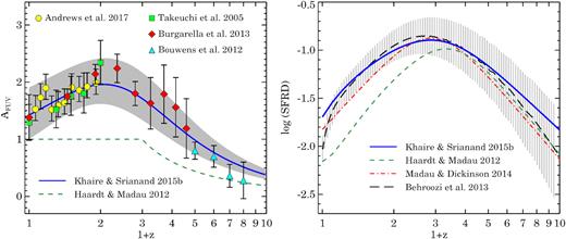
Left-hand panel: the average dust attenuation at FUV band (AFUV) in magnitudes with |$z$|. The solid-curve shows AFUV(|$z$|) used in our EBL (equation 15) and the grey-shaded region shows the range in the AFUV(|$z$|) arising from the scatter in the FUV luminosity functions of the galaxies (KS15b). Measurements by Andrews et al. (2017, circles) are obtained by fitting SEDs of a large number of galaxies. Data points from Takeuchi, Buat & Burgarella (2005, squares) and Burgarella et al. (2013, diamonds) were obtained using IRX-β relation on IR and FUV luminosity functions of the galaxies. Bouwens et al. (2012, triangles), in the measurements, used the slopes of high-|$z$| galaxy SEDs. We also show AFUV(|$z$|) used by HM12 (dash curve) for comparison. Right-hand panel: the SFRD(|$z$|) in units of |${\rm M_{\odot }\, yr^{-1}\, Mpc^{-3}}$|. The solid curve shows our fiducial SFRD(|$z$|) obtained using the AFUV(|$z$|) shown in the left-hand panel (equation 16). For comparison we also show the SFRD estimated by Madau & Dickinson (2014, dot-dash curve), Behroozi et al. (2013, big-dash curve), and by HM12 (small-dash curve). The vertical-striped region shows the 1σ uncertainty in the SFRD(|$z$|) from Behroozi et al. (2013). At |$z$| < 2 HM12 SFRD(|$z$|) is significantly different from others.
In the left-hand panel of Fig. 2, we show our AFUV(|$z$|) (solid-curve) along with their independent measurements obtained using the IRX-β relation (Takeuchi et al. 2005; Bouwens et al. 2012; Burgarella et al. 2013). Our AFUV(|$z$|) is also remarkably consistent with the recent measurements by Andrews et al. (2017) obtained by fitting SEDs to a large number of galaxies observed in GAMA and COSMOS surveys (see also Driver et al. 2016a). The grey-shaded region shows the uncertainty in the obtained AFUV(|$z$|) arising from the scatter in the reported far-UV GLFs (see KS15b). For comparison, we also show AFUV(|$z$|) used in HM12 for their UVB calculations, which is significantly smaller than the measurements and our values. The difference in AFUV(|$z$|) leads to different emissivities and SFRD(|$z$|), which can severely affect the estimates of the EBL as well as the required fesc to be consistent with |$\Gamma _{\rm H \, {\scriptscriptstyle I}}$| measurements. Our SFRD(|$z$|) obtained from the AFUV(|$z$|) and stellar population synthesis models is shown in the right-hand panel of Fig. 2. For comparison we also show the SFRD(|$z$|) obtained by HM12, Madau & Dickinson (2014), and Behroozi et al. (2013, scaled by a factor of 1.7 to match the differences in the IMF used). SFRD(|$z$|) of HM12 is significantly smaller than others due to the lower AFUV(|$z$|), as small as a factor of ∼3 at |$z$| < 2. At |$z$| < 6 our SFRD(|$z$|) agrees well with those of Behroozi et al. (2013) and Madau & Dickinson (2014) with differences smaller than 0.1 and 0.2 dex, respectively. At |$z$| > 6 our SFRD(z) is more owing to higher AFUV(|$z$|); however, within the 1σ uncertainty given by Behroozi et al. (2013) as shown by the striped region in the right-hand panel of Fig. 2 and also consistent with the SFRD(|$z$|) from very high-|$z$| GLFs (Oesch et al. 2014; Bouwens et al. 2015; McLeod et al. 2015).
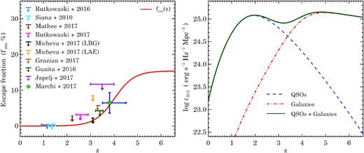
Left-hand panel: the average escape fraction fesc(|$z$|) of H|$\, \, {\rm {\scriptstyle I}}$| ionizing photons from galaxies used in our UVB code (solid-curve, equation 21). Various data points show the recent estimates of average fesc where downward arrows indicate 1σ upper limits. These points have been converted for our fiducial galaxy emissivity models as explained in the text and provided in Table A1. Horizontal bars on each point indicate the redshift range of the galaxy sample considered for measurements. Right-hand panel: the net specific emissivity at 912 Å (|$\epsilon _{\nu _{912}}$|) with |$z$| used in our fiducial UVB model (solid curve). The panel also shows the contribution from QSOs (dash-curve, see equation 14 for α = −1.8), galaxies (dot-dash curve, from equations 20 and 21 obtained for the fesc(|$z$|) shown in the left-hand panel) and the addition of both (solid curve).
In the right-hand panel of Fig. 3, we show the relative contribution of galaxies and QSOs to the extreme-UV emissivities, in terms of |$\epsilon_{912}(z)$|. We show QSO contribution |$\epsilon ^Q_{912}(z)$| for α = −1.8 and our galaxy contribution |$\epsilon ^G_{912}(z)$| (from equations 20 and 21). QSOs dominate the extreme-UV emissivity at |$z$| < 3 (irrespective of the assumed α value) and galaxies dominate at |$z$| > 3.5. The sharp increase and then saturation in |$\epsilon ^G_{912}(z)$| result from the fesc(|$z$|) adopted in our study (see the left-hand panel of Fig. 3). The rapid decrease in |$\epsilon ^Q_{912}(z)$| at |$z$| > 3 is the main reason for the required rapid increase in fesc(|$z$|) and hence in the |$\epsilon ^G_{912}(z)$| at 3.5 < |$z$| < 5.5 in order to be consistent with the ΓHi measurements (Khaire et al. 2016). If low-luminosity AGNs contribute appreciably to the emissivity at |$z$| > 3.5, as claimed by Giallongo et al. (2015), one may not need such a rapid increase in fesc(|$z$|) (see e.g. Khaire et al. 2016). We discuss the effect on UVB arising from uncertainties in galaxy emissivity in Section 4.4.2.
The galaxy emissivity obtained using equation (17) does not provide the IR and FIR emissivities since it includes only stellar radiation. Radiation from old stellar population peaks in near-IR around 1–3 μm and falls steeply at smaller wavelengths. Most of the observed FIR emissions from galaxies originate from the thermal emission of interstellar dust heated by UV and optical light from stars. We take the FIR emissivity estimated by KS15b for the same SFRD(|$z$|), AFUV(|$z$|), and the LMC2 extinction curve used here. It has been estimated under the assumption that the energy density absorbed by dust in UV and optical wavelengths is getting emitted in IR to FIR wavelengths and the spectral shape of this emission is similar to the one observed from galaxies in local Universe. Such a spectral shape has been taken from local IR galaxy templates of Rieke et al. (2009). This FIR emissivity has been shown to be consistent with various local observations. For more details on this, we refer readers to section 5 of KS15b.
3.3 Diffuse emissivity
Most of the gas in the IGM is in photoionization equilibrium with the UVB. This gas re-emits a fraction of energy it absorbs from the UVB at different wavelengths. This re-emission happens through various recombination channels such as Lyman-series and Lyman-continuum emission of H|$\, \, {\rm {\scriptstyle I}}$|, He|$\, \, {\rm {\scriptstyle I}}$|, and He|$\, \, {\rm {\scriptstyle II}}$|, similarly for Balmer and higher order series and continuum. Although it contributes negligibly to UVB as shown by FG09, we model few of the most dominant contributions in the extreme-UV wavelengths such as Lyman-continuum emission from H|$\, \, {\rm {\scriptstyle I}}$| and He|$\, \, {\rm {\scriptstyle II}}$|, Balmer-continuum emission from He|$\, \, {\rm {\scriptstyle II}}$| and the Lyman-α emission from He|$\, \, {\rm {\scriptstyle II}}$| following the procedure in FG09 and HM12. We briefly describe it here. For more details, we refer readers to the relevant sections in FG09 and HM12.
We have also modeled the H|$\, \, {\rm {\scriptstyle I}}$| Lyman-α emissivity from galaxies, which is not included in the population synthesis models. For this we followed the simple procedure used by HM12 (their section 7.1), which assumes that 68 per cent of the Lyman continuum photons that are not able to escape the galaxies [i.e. (1 − fesc) × 0.68] are being emitted as Lyman-α photons. Unlike HM12, we multiply this H|$\, \, {\rm {\scriptstyle I}}$| Lyman-α emissivity by |$10^{-0.4A_{\rm FUV}(z)D_{Ly\alpha }/D_{\rm FUV}}$| to capture the effect of the dust attenuation. Therefore, our UVB does not show prominent Lyman-α emission as compared to HM12. Note that such a simple method to estimate the H|$\, \, {\rm {\scriptstyle I}}$| Lyman-α emissivity may not be consistent with the complex radiative transfer and escape of Lyman-α photons emitted by stellar population through ISM and CGM of galaxies (see e.g. Neufeld 1990, 1991; Dijkstra, Haiman & Spaans 2006; Dayal, Ferrara & Saro 2010; Gronke et al. 2016; Dijkstra 2017).
4 BASIC RESULTS
In this section we discuss basic results from our fiducial model (Q18 model with α = −1.8 used in QSO SED) for the photoionization and photoheating rates of H|$\, \, {\rm {\scriptstyle I}}$| and He|$\, \, {\rm {\scriptstyle II}}$|, the reionization history of H|$\, \, {\rm {\scriptstyle I}}$| and He|$\, \, {\rm {\scriptstyle II}}$|, the spectrum of local EBL from FIR to γ-rays, and the UVB spectrum along with its comparison with models of FG09 and HM12. Similar results for the models obtained with different α are presented in Appendix E. We also discuss the uncertainties in the UVB arising from different model parameters.
4.1 Photoionization and photoheating rates
The photoionization rates of H|$\, \, {\rm {\scriptstyle I}}$| and He|$\, \, {\rm {\scriptstyle II}}$| are the only observed constraints on the UVB. Moreover, these are just integral constraints and can decide the intensity of the UVB if only the spectral shape of the UVB is known. However, unlike the direct observational constraints on EBL at wavelengths other than extreme-UV, photoionization rates are not limited to the local Universe and can be measured across a large redshift range using various observational techniques as mentioned in Section 1. In our analysis, we use the recent |$\Gamma _{\rm H \, {\scriptscriptstyle I}}$| measurements obtained by comparing the cosmological simulations of the IGM to the observed statistics of the Ly-α forest by Gaikwad et al. (2017a) at |$z$| < 0.5, by Becker & Bolton (2013) and Bolton & Haehnelt (2007) at 2 < |$z$| < 5, and by D’Aloisio et al. (2018) and Wyithe & Bolton (2011) at 5 < |$z$| < 6. We also use the |$\Gamma _{\rm H \, {\scriptscriptstyle I}}$| measurements obtained from proximity zones of high-|$z$| QSOs by Calverley et al. (2011) at |$z$| = 5 and 6.1. In addition to |$\Gamma _{\rm H \, {\scriptscriptstyle I}}$|, we have also used the |$\Gamma _{\rm He \, {\scriptscriptstyle II}}$| measurements by Khaire (2017).
In the left-hand panel of Fig. 4, we show |$\Gamma _{\rm H\, {\scriptscriptstyle I}}(z)$| obtained from our fiducial UVB model along with various available measurements. The remarkable agreement between our prediction and the |$\Gamma _{\rm H \, {\scriptscriptstyle I}}$| measurements at |$z$| > 3 is not surprising since we have chosen the appropriate fesc(|$z$|) to match these measurements (see Khaire et al. 2016). Whereas, at |$z$| < 3, the UVB is determined by our updated QSO emissivity alone (see also KS15a) and there is no need to adjust fesc(|$z$|). However, for making fesc(|$z$|) as a continuous function of |$z$|, we have taken negligibly small values of fesc(|$z$|) at |$z$| < 2.5. At |$z$| < 0.5, our |$\Gamma _{\rm H \, {\scriptscriptstyle I}}$| is consistent not only with measurements from Gaikwad et al. (2017a) but also with Shull et al. (2015), Gurvich et al. (2017), Viel et al. (2017), Khaire et al. (2018), and Fumagalli et al. (2017), which are not shown in the figure due to shortage of space. The |$z$| = 0 Fumagalli et al. (2017) measurement is obtained using the observations of Hα fluorescence from a nearby faint disc galaxy. Note that all these |$z$| < 0.5 measurements provide ∼2.5 times smaller |$\Gamma _{\rm H \, {\scriptscriptstyle I}}$| than the measurements of Kollmeier et al. (2014). For comparison, we also show |$\Gamma _{\rm H\, {\scriptscriptstyle I}}(z)$| obtained in UVB models of HM12, FG09,3 and a new model of Puchwein et al. (2019). At |$z$| < 0.5, unlike our models the previous two models by HM12 and FG09 underpredict |$\Gamma _{\rm H \, {\scriptscriptstyle I}}$| values compared to latest measurements. This is one of our major improvements over these previous UVB models. The differences in |$\Gamma _{\rm H\, {\scriptscriptstyle I}}(z)$| predicted by these models at |$z$| > 2 are because of choosing different inputs in their UVB models, such as fesc, in order to be consistent with different |$\Gamma _{\rm H\, {\scriptscriptstyle I}}(z)$| measurements. For example, FG09 tried to be consistent with |$\Gamma _{\rm H\, {\scriptscriptstyle I}}(z)$| from Faucher-Giguère et al. (2008), whereas HM12 with |$\Gamma _{\rm H\, {\scriptscriptstyle I}}(z)$| from Becker, Rauch & Sargent (2007), which are quite different from the recent measurements (see Becker & Bolton 2013, for more details). Overall, our |$\Gamma _{\rm H\, {\scriptscriptstyle I}}(z)$| values are in excellent agreement with the recent measurements at all redshifts than previous UVB models. The |$\Gamma _{\rm H \, {\scriptscriptstyle I}}$| predicted by the new UVB model of Puchwein et al. (2019) is also in very good agreement with recent measurements and our model predictions at |$z$| < 5.5. This new model has employed a novel opacity treatment to synthesize UVB in the pre-H|$\, \, {\rm {\scriptstyle I}}$| and He|$\, \, {\rm {\scriptstyle II}}$|-reionization era following Madau & Fragos (2017). A sharply decreasing |$\Gamma _{\rm H\, {\scriptscriptstyle I}}(z)$| at |$z$| > 5.8 is one of the by-products of such opacity treatment that has been shown to be important in reproducing reionization history and heating in hydrodynamical simulations of the IGM (see also Oñorbe, Hennawi & Lukić 2017a). However, the success of Puchwein et al. (2019) at |$z$| < 1 to reproduce recent |$\Gamma _{\rm H \, {\scriptscriptstyle I}}$| measurements mainly comes from using updated QSO emissivity similar to our model (see also Madau & Haardt 2015). Note that the uncertainties in the |$\Gamma _{\rm H \, {\scriptscriptstyle I}}$| measurements are different for different measurement methods. Even for the same method, such as using flux decrement, the uncertainties depend on choice of range in the thermal state of the IGM used in calculation (see D’Aloisio et al. 2018). Therefore, the agreement between UVB models and the |$\Gamma _{\rm H \, {\scriptscriptstyle I}}$| measurements also depends on the |$\Gamma _{\rm H \, {\scriptscriptstyle I}}$| measurements considered in the model.
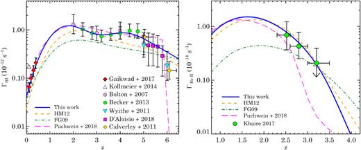
The photoionization rate of H|$\, \, {\rm {\scriptstyle I}}$| (ΓHi; left-hand panel) and He|$\, \, {\rm {\scriptstyle II}}$| (ΓHe ii; right-hand panel) as a function of |$z$| from our fiducial UVB model (solid curves; see Fig. E1 for UVB models with different α). For comparison we show the ΓHi from UVB models of HM12 (small-dash curve) and FG09 (dot-dash curve) and new model by Puchwein et al. (2019, big-dash curve). Various data points in the left-hand panel show the recent measurements of ΓH i. The ΓHe ii from Khaire (2017) is obtained by using the measurements of |$\tau _{\alpha }^{\rm He II}$| from Worseck et al. (2016).
UVB models with different α give slightly different values of |$\Gamma _{\rm H \, {\scriptscriptstyle I}}$| at |$z$| < 3 because at these redshifts the UVB is dominated by QSOs. However, these are still consistent with the measurements of Gaikwad et al. (2017a) as shown in the left-hand panel of Fig. E1 in the Appendix. This shows that the difference in the obtained |$\Gamma _{\rm H \, {\scriptscriptstyle I}}$| due to changing α (from −1.4 to −2) is smaller than the present uncertainties on the low-|$z$||$\Gamma _{\rm H \, {\scriptscriptstyle I}}$| measurements. At |$z$| > 3, |$\Gamma _{\rm H \, {\scriptscriptstyle I}}$| is dominated by galaxy emissivity, therefore the left-hand panel of Fig. E1 does not show any change in |$\Gamma _{\rm H \, {\scriptscriptstyle I}}$| with α.
In the right-hand panel of Fig. 4, we show |$\Gamma _{\rm He \, {\scriptscriptstyle II}}(z)$| obtained from our fiducial UVB along with the values determined in Khaire (2017) at 2.5 < |$z$| < 3.5 by using the He|$\, \, {\rm {\scriptstyle II}}$| effective optical depth measurements of Worseck et al. (2016) and the f(NH i, |$z$|) from Inoue et al. (2014). For comparison, we also show the |$\Gamma _{\rm He \, {\scriptscriptstyle II}}(z)$| from UVB models of HM12, FG09 and a new model of Puchwein et al. (2019). |$\Gamma _{\rm He \, {\scriptscriptstyle II}}(z)$| obtained by our and HM12 UVB models match very well with the measurements. In this |$z$|-range where direct observations are available, the |$\Gamma _{\rm He \, {\scriptscriptstyle II}}(z)$| from FG09 and Puchwein et al. (2019) are also broadly consistent with Khaire (2017) measurements. The agreement between our and HM12,|$\Gamma _{\rm He \, {\scriptscriptstyle II}}$| at 2.5 < |$z$| < 3.5, despite the fact that we are using different input parameters, is mostly coincidental and because of using different QSO SEDs. HM12 used smaller |$\epsilon ^Q_{1000}$| but steeper SED (α = −1.57), on the other hand we used higher |$\epsilon ^Q_{1000}$| but shallower SED (α = −1.8). Also, the fact that both models get almost the same |$\Gamma _{\rm H \, {\scriptscriptstyle I}}$| within 2.5 < |$z$| < 3.5 helps in getting the |$\Gamma _{\rm He \, {\scriptscriptstyle II}}(z)$| agreement.
|$\Gamma _{\rm He \, {\scriptscriptstyle II}}$| is more sensitive to the value of α than |$\Gamma _{\rm H \, {\scriptscriptstyle I}}$|. It is because α is obtained by normalizing QSO emissivity at λ = 1000 Å. Therefore, a small change in α results in a large change for He|$\, \, {\rm {\scriptstyle II}}$| ionizing photons at more than four times smaller wavelengths. We show |$\Gamma _{\rm He \, {\scriptscriptstyle II}}$| obtained from our UVB models with different α in the right-hand panel of Fig.E1. Only −2.0 < α < −1.6 are consistent with the |$\Gamma _{\rm He \, {\scriptscriptstyle II}}$| measurements and He|$\, \, {\rm {\scriptstyle II}}$| effective optical depths (for more detailed analysis on this, refer to Khaire 2017). We note that new measurements of |$\Gamma _{\rm He \, {\scriptscriptstyle II}}(z)$| by Worseck et al. (2018) are consistent with our UVB predictions for α = −2.0.
4.2 H|$\, \, {\rm {\scriptstyle I}}$| and He|$\, \, {\rm {\scriptstyle II}}$| reionization
We show the QHii(|$z$|) and QHe iii(|$z$|) results in the left-hand panel of Fig. 5. We also show recent measurements of QHii. H|$\, \, {\rm {\scriptstyle I}}$| reionization in our model completes at |$z$| = 5.8 (|$z$| at which Qx(|$z$|) = 1) consistent with high-|$z$| Lyman-α forest observations (Becker et al. 2001; Fan et al. 2006). Our QH ii(|$z$|) is in agreement with lower limits from McGreer et al. (2015) obtained using dark-pixel statistics of high-z QSO spectra and with measurements of Greig et al. (2017) and Bañados et al. (2018) obtained using Lyman-α damping wings of two highest redshift QSOs. Our QHii(|$z$|) is also consistent with the measurements obtained from the diminishing population of high-|$z$| Lyman-α emitters obtained by Schenker et al. (2014), Mason et al. (2018), and Inoue et al. (2018). We calculate the electron scattering optical depth τe of CMB (equation 12 from Khaire et al. 2016). The τe(|$z$|) from our reionization model is shown in the central panel of Fig. 5, which reaches asymptotic value τe = 0.55 consistent with the measurements of Planck Collaboration XLVI (2016b). This reiterated the results of Khaire et al. (2016) that new constraints on H|$\, \, {\rm {\scriptstyle I}}$| reionization do not require fesc(|$z$|) at |$z$| > 6 to have a steep evolution and a constant value, such as 0.15 used here (equation 21), is sufficient to produce the consistent τe. The H|$\, \, {\rm {\scriptstyle I}}$| reionization history is same for all of our UVB models obtained with different α because in these models the H|$\, \, {\rm {\scriptstyle I}}$| reionization is driven by galaxies and QSOs contribute negligibly.
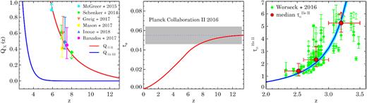
Left-hand panel: volume filling fraction of H|$\, \, {\rm {\scriptstyle II}}$| (red curve) and He|$\, \, {\rm {\scriptstyle III}}$| (blue curve) obtained for our fiducial UVB model. For comparison the QHii measurements from Schenker et al. (2014), McGreer et al. (2015), Greig et al. (2017), Mason et al. (2018), Bañados et al. (2018), and Inoue et al. (2018) have been shown. We get |$z$|re = 5.8 for H|$\, \, {\rm {\scriptstyle I}}$| and |$z$|re = 2.8 for He|$\, \, {\rm {\scriptstyle II}}$|. Central panel: electron scattering optical depth (τe) obtained from our fiducial UVB model (solid curve) shown together with the measurements from Planck Collaboration XLVI (2016b, dotted line with grey shade). Right-hand panel: the He|$\, \, {\rm {\scriptstyle II}}$| Lyman-α effective optical depth (|$\tau _{\rm \alpha }^{\rm He\, {\scriptscriptstyle II}}$|) obtained from our fiducial UVB model (solid curves with b = 28 km s−1 and cyan shade obtained by changing b from 24 to 32 km s−1) with the measurements from Worseck et al. (2016, diamonds). The red points show the median |$\tau _{\alpha }^{\rm He II}$| in redshift bins indicated by horizontal bars.
He|$\, \, {\rm {\scriptstyle II}}$| reionization in our fiducial model with α = −1.8 completes at |$z$| = 2.8. It is consistent with various measurements of He|$\, \, {\rm {\scriptstyle II}}$| Lyman-α effective optical depths (|$\tau _{\rm \alpha }^{\rm He\, {\scriptscriptstyle II}}$|; Kriss et al. 2001; Shull et al. 2004, 2010; Fechner et al. 2006; Worseck et al. 2011, 2016), measurements of peak in the redshift evolution of mean IGM temperature (Becker et al. 2011; Hiss et al. 2018) and also with theoretical models of He|$\, \, {\rm {\scriptstyle II}}$| reionization (McQuinn et al. 2009; Compostella, Cantalupo & Porciani 2013; La Plante & Trac 2016). We also consistently reproduce |$\tau _{\rm \alpha }^{\rm He\, {\scriptscriptstyle II}}$| from Worseck et al. (2016), as shown in the right-hand panel of Fig. 5. It shows |$\tau _{\rm \alpha }^{\rm He\, {\scriptscriptstyle II}}$| calculated from our fiducial UVB model (using equations 9 and 10 from Khaire 2017) for an assumed Doppler broadening b = 28 km s−1 with blue curve and the shaded cyan region provides values encompassed by changing b from 24 to 32 km s−1. The red data points, shown to guide the eyes, are the median values of |$\tau _{\rm \alpha }^{\rm He\, {\scriptscriptstyle II}}$| (within 95 percentile errors) as obtained in three different |$z$| bins (see table 2 of Khaire 2017). Note that the He|$\, \, {\rm {\scriptstyle II}}$| reionization history and |$\tau _{\rm \alpha }^{\rm He\, {\scriptscriptstyle II}}$|(|$z$|) depends on the value of α. As shown in Khaire (2017), only −2.0 < α < −1.6 are consistent with both |$\tau _{\rm \alpha }^{\rm He\, {\scriptscriptstyle II}}$| measurements and epoch of He|$\, \, {\rm {\scriptstyle II}}$| reionization being 2.6 < |$z$| < 3.0. Similar conclusions are presented in the recent study by Gaikwad et al. (2018a) using the UVB models presented here in hydrodynamic simulations of the IGM explicitly taking into account the non-equilibrium ionization effects.
4.3 The EBL spectrum
In Fig. 6, we show our full EBL spectrum at |$z$| = 0. Our calculations cover more than 15 orders of magnitude range in wavelength from FIR to TeV energy γ-rays. The three distinct peaks in the intensity, 4πνJν in units of erg s−1 cm−2, can be readily seen. These are the FIR peak arising from the dust emission around ∼100 μm (106 Å), the near-IR peak dominated by old stellar population around ∼1 μm (104 Å) and the hard X-ray peak from type 2 QSOs around ∼30 keV (0.4 Å). In general, the λ > 912 Å part of the EBL is dominated by emission from galaxies including their stellar and dust emission, the λ < 228 Å part is contributed by radiation only from QSOs, and the 912 > λ > 228 Å part is contributed by both galaxies and QSOs. Relative contribution to the latter is determined by fesc, which at |$z$| = 0 is negligibly small; therefore, it is contributed by QSOs alone.

In Fig. 6, we also show |$z$| = 0 EBL measurements at different wavelengths obtained by various methods and instruments. In the FIR wavelengths we use compiled measurements by Dwek & Krennrich (2013, their table 7) obtained from COBE. In the optical to FIR wavelengths we use compiled measurements by Kneiske & Dole (2010) and Driver et al. (2016b) obtained from integrated light from resolved galaxies in deep surveys. Our EBL models agree very well with these measurements. At 0.25 keV (λ ∼ 50 Å) the measurement is taken from Warwick & Roberts (1998) obtained using shadow measurements from ROSAT. The X-ray background measurements are taken from various instruments; Chandra (Cappelluti et al. 2017), ASCA (Gendreau et al. 1995), HEAO-1 and HEAO-4 (Gruber et al. 1999; Kinzer et al. 1997), Integral (Churazov et al. 2007), RXTE (Revnivtsev et al. 2003), Swift/BAT (Ajello et al. 2008), and Nagoya balloon (Fukada et al. 1975). Similarly γ-ray background measurements are taken from instruments: SMM (Watanabe et al. 1997), compton/Comptel (Weidenspointner et al. 2000), compton/EGRET (Strong, Moskalenko & Reimer 2003), and Fermi/LAT (Ackermann et al. 2015). Our local fiducial EBL shows remarkable match with the X-ray and γ-ray background measurements all the way upto TeV γ-rays. It is not surprising, since we have constructed type 2 QSO and blazar SED (Section 3.1) and adjusted the normalizations (see Table 1) to do so. In Fig. E3, we show our EBL models with different values of α. The normalization hν0 and Sk are taken such that despite different α, the local EBL will consistently reproduce the X-ray and γ-ray measurements as shown in Fig. E3. However, with our assumed QSO SED shape, it becomes difficult for models with α > −1.5, to match few of the soft X-ray measurements.
The optical depth encountered by high-energy γ-rays (τγ) due to EBL is discussed in Appendix C. We find that τγ is insensitive to EBL at E < 10 eV and thus to values of α. Note that the EBL at E < 10 eV is same as the fiducial model given in KS15b (the median LMC2 model) and therefore it is consistent with many published models of optical and FIR EBL (e.g. Franceschini, Rodighiero & Vaccari 2008; Finke, Razzaque & Dermer 2010; Kneiske & Dole 2010; Domínguez et al. 2011; Gilmore et al. 2012; Helgason & Kashlinsky 2012; Inoue et al. 2013; Scully, Malkan & Stecker 2014) as shown in KS15b. We provide the updated τγ values calculated for our fiducial EBL model including CMB.
The UVB at z = 0, a part of the EBL at 50 < λ < 1200 Å (i.e. 10 < E < 250 eV) shown in Fig. 6, does not have any direct measurements. The measurements such as photoionization rates provide only integral constraints. Our models are consistent with them across a large |$z$|-range as shown in Fig. 4. Below we discuss the UVB spectrum and its redshift evolution in comparison with the previous UVB models. For the discussions hereafter, let us naively divide the EBL at λ < 912 Å (E > 13.6 eV) into three parts, the H|$\, \, {\rm {\scriptstyle I}}$| ionizing UVB at 13.6 < E < 54.4 eV, the He|$\, \, {\rm {\scriptstyle II}}$| ionizing UVB at 54.4 < E < 500 eV, and the X-ray background at E > 500 eV.
In Fig. 7, we compare our fiducial UVB spectrum from |$z$| = 0 to 5 with the UVB from FG09 and HM12. Two distinct features in the UVB spectrum can be readily seen; these are ionization edges of H|$\, \, {\rm {\scriptstyle I}}$| (at 13.6 eV) and He|$\, \, {\rm {\scriptstyle II}}$| (at 54.4 eV). The smoothness of these features at the bottom of the troughs is because of the inclusion of Lyman continuum emission from H|$\, \, {\rm {\scriptstyle I}}$| and He|$\, \, {\rm {\scriptstyle II}}$| in UVB calculations. Also, there is a small kink at 40.8 eV, prominent at |$z$| = 1 to 4 UVB, due to He|$\, \, {\rm {\scriptstyle II}}$| Lyman-α recombination emission. Another such small kink due to H|$\, \, {\rm {\scriptstyle I}}$| Lyman-α recombination emission from galaxies at 10.2 eV can be seen in HM12 but not in our UVB, because this emission is suppressed in our models due to dust correction. FG09 do not include H|$\, \, {\rm {\scriptstyle I}}$| Lyman-α recombination emission in their calculations. Sharp saw-tooth features due to Lyman series absorption of He|$\, \, {\rm {\scriptstyle II}}$|, seen in HM12 UVB at |$z$| > 3, are not included in our and FG09 models. Note that this saw-tooth modulation only shows significant difference in UVB at high redshifts and affects a very small wavelength range.

The differences in the UVB models can be roughly mapped to the differences in their predictions of |$\Gamma _{\rm H \, {\scriptscriptstyle I}}$| and |$\Gamma _{\rm He \, {\scriptscriptstyle II}}$| (see Fig. 4). The UVB model of FG09 is significantly different from our and HM12 model at all wavelengths and redshifts. Our UVB model at |$z$| < 2 has higher H|$\, \, {\rm {\scriptstyle I}}$| ionizing UVB as compared to both FG09 and HM12 models. At |$z$| < 1, the similar He|$\, \, {\rm {\scriptstyle II}}$| ionizing UVB seen for ours and HM12 model is because of the coincidental combinations of different α and |$\epsilon _{\nu }^Q$| used in both models. At higher redshifts our He|$\, \, {\rm {\scriptstyle II}}$| ionizing UVB shows larger deviation from HM12. The similarity of X-ray background in our and HM12 at |$z$| = 0 is due to the fact that both models match the X-ray background measurements, which was not attempted by FG09. The He|$\, \, {\rm {\scriptstyle II}}$| ionizing UVB in FG09 shows comparatively smaller intensities with larger troughs at |$z$| < 2, suggesting that He|$\, \, {\rm {\scriptstyle II}}$| is recombining quickly in their model. This is not surprising given the small recombination time-scales of He|$\, \, {\rm {\scriptstyle II}}$|, the ever-decreasing |$\Gamma _{\rm He \, {\scriptscriptstyle II}}$| at |$z$| < 2 and their small values at higher |$z$| > 2 (see the right-hand panel of Fig. 4). Sources of all these significant differences among the three UVB models are the differences in the input parameters used in modeling, mainly the emissivities from QSOs and galaxies along with the |$\Gamma _{\rm H \, {\scriptscriptstyle I}}$| measurements that are used to check or calibrate the models.
The significant differences in the UVB models highlight the need for routinely updating the models using ever-improving measurements of important input parameters. It is also important that the photoionization calculations that depend extensively on the assumed UVB model should use updated UVB keeping in mind all the uncertainties involved in the calculations of UVB. This is the main reason why we provide six other UVB models having different α values than our fiducial model. For these models, the differences in the obtained UVB spectrum can be seen from Fig. E4 of the Appendix. The intensity of He|$\, \, {\rm {\scriptstyle II}}$| ionizing UVB increases with α at all |$z$| since it depends only on QSO emissivity, on the other hand the H|$\, \, {\rm {\scriptstyle I}}$| ionizing UVB depends on both QSOs and galaxies, therefore it only shows clear dependences on α for |$z$| < 3 where QSOs are dominating the UVB. As mentioned earlier, the intensity of He|$\, \, {\rm {\scriptstyle II}}$| ionizing UVB is more sensitive to α than H|$\, \, {\rm {\scriptstyle I}}$| ionizing UVB, as can be seen from Fig. E4 of the Appendix for UVB at |$z$| < 3. We make all these UVBs publicly available for testing the dependence of photoionization calculation results on the assumed spectral shape of the UVB and to be able to quantify the uncertainties in the inferred quantities from these calculations. In the following section, we give a detailed account of the uncertainties involved in the UVB calculations.
4.4 Uncertainties and caveats in the UVB models
The synthesis models of EBL are affected by several assumptions and many uncertainties arising from various input parameters. Here, we discuss such uncertainties and caveats in our UV and X-ray background models (E > 13.6 eV). We refer interested readers to section 9 of KS15b for the discussion related to uncertainties in the far-UV to FIR parts (E < 13.6 eV) of the EBL.
4.4.1 QSO emissivity and SED
Uncertainties in QSO emissivity arise from how well we measure the QLF (especially at low luminosities) and how representative is the SED used in the wavelength range where there are no direct observations. At |$z$| < 2 the QLFs are relatively well measured having shallow faint end slopes. Therefore, uncertainties in the obtained emissivity at |$z$| < 2 by integrating down to faintest luminosity are small. For example, for |$z$| < 2 QLFs from Croom et al. (2009) and Palanque-Delabrouille et al. (2013), changing the minimum luminosity |$L_{\nu }^{\rm min}=0.01L^*$| to |$L_{\nu }^{\rm min}=0$| changes the emissivity by less than 5 per cent. Although we are using most recent measurements, the |$z$| > 3 QLFs at the low luminosities are not well-measured, which can make our assumed emissivities highly uncertain at these redshifts.
For a fixed type 1 QSO SED, any effect of a change in QSO emissivity will be compensated by a corresponding change in the fesc to match the |$\Gamma _{\rm H \, {\scriptscriptstyle I}}$| measurements. However, this required change in fesc can affect the spectral shape of the H|$\, \, {\rm {\scriptstyle I}}$| ionizing UVB depending on the differences in the type 1 QSO SED and the intrinsic SED of galaxies at E > 13.6 eV. Latter is obtained from stellar population synthesis models. For our fiducial UVB model, since the SED of QSOs (with α = −1.8) is co-incidentally same as our intrinsic SED of galaxies, using different QSO emissivity will not affect even the spectral shape of H|$\, \, {\rm {\scriptstyle I}}$|-ionizing UVB. However, the He|$\, \, {\rm {\scriptstyle II}}$|-ionizing UVB will be affected since it depends on the emission from type 1 QSOs and the |$\Gamma _{\rm H \, {\scriptscriptstyle I}}$| through radiative transfer effects that determine η (see Khaire 2017).4 For example, there is no need to have a seemingly unrealistic sharp increase in fesc with |$z$| (see the left-hand panel of Fig. 3) if the QSO emissivity is significantly higher than our fiducial values at |$z$| > 3.5. A much slower or no evolution in fesc(|$z$|) can be easily achieved as shown in Khaire et al. (2016) when one uses high QSO emissivity models based on the QLF measurements by Giallongo et al. (2015) and assuming that the low-luminosity QSOs also have high (close to unity) escape fraction (see Grazian et al. 2018). However, such models have serious problems to reproduce the He|$\, \, {\rm {\scriptstyle II}}$| optical depth as a function of |$z$| (Khaire 2017). Moreover QLF measurements of Giallongo et al. (2015) are not supported by other similar studies (see e.g. Weigel et al. 2015; McGreer et al. 2018; Ricci et al. 2017)
Even the latest measurements of type 1 QSO SED show large variation in the measured value of power-law index α at E > 13.6 eV (from −2.3 to −0.5 within 1σ errors; Stevans et al. 2014; Lusso et al. 2015; Tilton et al. 2016). See table 1 of Khaire (2017) for a summary of α measurements till date. The change in H|$\, \, {\rm {\scriptstyle I}}$| ionizing UVB arising due to change in α can be seen in Fig. E4 for |$z$| ≤ 2, where the UVB is dominated by only type 1 QSOs. At |$z$| > 3, Fig. E4 shows no variation in H|$\, \, {\rm {\scriptstyle I}}$| ionizing UVB with change in α since it is dominated by emission from galaxies. The He|$\, \, {\rm {\scriptstyle II}}$| ionizing part of the UVB, however, shows a large variation with α at all redshifts, since it only depends on type 1 QSO emissivity. The existing measurements of α probe smallest wavelength only upto 425 Å (30 eV), therefore there are no direct observational constraints on QSO SED at He|$\, \, {\rm {\scriptstyle II}}$| ionizing wavelengths. It has been assumed that the type 1 QSO SED at λ < 912 Å (E > 13.6 eV) follows a single power law (with same α), which is normalized at 912 Å or higher wavelengths. This extrapolated power law to He|$\, \, {\rm {\scriptstyle II}}$| ionizing wavelengths gives large-intensity differences corresponding to small changes in α. Therefore, He|$\, \, {\rm {\scriptstyle II}}$| ionizing UVB and |$\Gamma _{\rm He \, {\scriptscriptstyle II}}(z)$| are more sensitive to α values than the H|$\, \, {\rm {\scriptstyle I}}$| ionizing UVB and |$\Gamma _{\rm H\, {\scriptscriptstyle I}}(z)$| as can be observed from Figs E1 and E4 of the Appendix. Under the assumption of a single power law, in Khaire (2017) we find that α can have values from −1.6 to −2.0 consistent with measurements of Lusso et al. (2015) but smaller than measurements of Stevans et al. (2014) and Tilton et al. (2016). We provide UVB models with varying α from −1.4 to −2.0 in Appendix E. Using different α in the UVB models can affect the inferred properties of absorbers in the IGM and CGM, such as metallicity (Hussain et al. 2017; Muzahid et al. 2018), density (Hussain et al. 2017; Upton Sanderbeck et al. 2018), and temperatures (Gaikwad et al. in preparation).
Type 2 QSO SED and its normalizations, for different values of α used in type 1 QSO SED (see Table 1) are adjusted to be consistent with most of the X-ray and γ-ray background measurements at |$z$| = 0. These models with different α are shown in Fig. E3. For large values of α, such as −1.4 or −1.5, it is difficult to adjust normalizations to be consistent with some of the soft X-ray measurements. Nevertheless, all models are consistent with measurements at energies more than 20 keV all the way upto TeV. Although this shows a major success of such type 2 QSO and blazar SED formulation, it has been assumed to scale with type 1 QSO emissivity, with the same scaling at all redshifts. Such scaling can be justified using recent observations of QSO population (Lusso et al. 2013; Georgakakis et al. 2017; Vito et al. 2018), where the fraction of type 2 QSOs is shown to be non-evolving with redshift (however, see Gohil & Ballantyne 2018; Liu et al. 2017). Due to this scaling, all the uncertainties in type 1 QSO emissivity reflect in the normalization of type 2 QSO SED. Although it will not affect the obtained X-ray background, it will change the interpretation related to the fraction of type 2 QSOs as discussed in Appendix D. However, one should take such an interpretation with caution since the type 1 and type 2 QSO SEDs at X-ray can be adjusted arbitrarily to give different fractions of type 2 QSOs while still being consistent with local X-ray and γ-ray background measurements.
The soft-X-ray background (0.3 keV < E < 2 keV) in our EBL model is contributed only by QSOs. However, as shown in Upton Sanderbeck et al. (2018), a significant contribution at |$z$| ∼ 0 can come from hot intra-halo gas. The contribution from interstellar gas, CGM, and X-ray binary is relatively small; however, it depends on the SFRD used in the models. Upton Sanderbeck et al. (2018) used SFRD from HM12, which is a factor of ∼3 smaller than other estimates at |$z$| < 1. In our EBL models we have not included soft-X-ray background arising from these different sources that, when included in EBL models, can further constrain the SED of type 1 and 2 QSOs and can also change the interpretation of fraction of type 2 QSOs as mentioned above.
4.4.2 Galaxy emissivity and escape fraction
The emissivity of galaxies at λ < 912 Å depends, in addition to the intrinsic emissivity, on fesc. In our model by construct fesc is constrained to reproduce the H|$\, \, {\rm {\scriptstyle I}}$| ionizing UVB consistent with |$\Gamma _{\rm H \, {\scriptscriptstyle I}}$| measurements. The intrinsic emissivity at λ < 912 Å depends on the derived SFRD and AFUV as well as several parameters in the stellar population models. The derived SFRD and AFUV alone can have systematic uncertainties of the order of 30 per cent arising due to scatter in various FUV GLFs (see e.g. figs 1 and 5 of KS15b). Uncertainties arising in SFRD and AFUV from different parameters in stellar population models, such as using different metallicity, are smaller than this uncertainty (see section 8.2 of KS15b for more details).
As long as the intrinsic SED of galaxies at λ < 912 Å is same, the intensity of H|$\, \, {\rm {\scriptstyle I}}$| ionizing UVB remains same for different inferred values of fesc arising from different values of SFRD, AFUV, IMF, metallicity, or other parameters in the stellar population model. This is because in the UVB calculations the intrinsic galaxy SED has been scaled with fesc (see also HM12, FG09), in the absence of any observational constraints on the SED of emitted light from galaxies at λ < 912 Å. Such a scaling is justified under the assumption that these photons escape through gas and dust free channels, as proposed in many theoretical models (e.g. Fujita et al. 2003; Gnedin et al. 2008; Paardekooper et al. 2011; Conroy & Kratter 2012). Although the intrinsic SED at λ < 912 Å shows reasonably small variations for different properties of stellar populations such as metallicity (see section 4 of Becker & Bolton 2013) and different synthesis models (see section 9 of HM12), different IMFs can provide quite different intrinsic SEDs.
If independent constraints on fesc are available, then the above-mentioned uncertainties will translate to uncertainties in the UVB spectrum. In our models, for a given QSO emissivity, the fesc values are adjusted to match |$\Gamma _{\rm H \, {\scriptscriptstyle I}}$| measurements in the absence of strong constraints on the fesc measurements. In future, independent constraints on fesc or H|$\, \, {\rm {\scriptstyle I}}$| ionizing emissivity will be useful to quantify the contributions of sources other than QSOs and galaxies to the UVB.
4.4.3 H|$\, \, {\rm {\scriptstyle I}}$| distribution and other uncertainties
The column density distribution of the H|$\, \, {\rm {\scriptstyle I}}$|, f(NH i, |$z$|) plays an important role in shaping the UVB model. The f(NHi, |$z$|) affects UVB estimate through the calculation of τeff, especially at |$15\lt {\rm log}(N_{\rm H\,{\small I} } \, \, {\rm cm^{-2}})\lt 20.5$| for H|$\, \, {\rm {\scriptstyle I}}$| ionizing UVB (see Fig. 8) and 4/η times values for He|$\, \, {\rm {\scriptstyle II}}$| ionizing UVB. This |$N_{\rm H\,{\small I}}$| range has relatively higher measurement uncertainty as compared to log|$(N_{\rm H\,{\small I}} \, \, {\rm cm^{-2}})\lt 14$| or >20 due to saturation of the Lyman-α absorption. We have used a f(NHi, |$z$|) fitting form provided by Inoue et al. (2014) because it has been obtained by fitting a large number of different observations covering large redshift and |$N_{\rm H\,{\small I}}$| range, as mentioned in Section 2. For comparison, in the left-hand panel of Fig. 8, we show the f(NH i, |$z$|) measurements at |$z$| = 2.5 along with the fitting forms from Inoue et al. (2014), FG09, and HM12. The fit from Inoue et al. (2014) is better than others at all |$N_{\rm H\, {\rm {\scriptstyle I}}}$|. The difference in the obtained τeff at each |$N_{\rm H\,{\small I}}$| for different f(NHi, |$z$|) fits are shown in the right-hand panel of Fig. 8, where a contribution of τeff at each |$N_{\rm H\,{\small I}}$| is represented by quantity NH if(NHi, |$z$|)[1 − exp(− NHiσ912)]. When we use the f(NHi, |$z$|) from HM12 instead of Inoue et al. (2014), at |$z$| < 3 our |$\Gamma _{\rm H \, {\scriptscriptstyle I}}$| reduces by 10 per cent (at |$z$| ∼ 2.5 and by 25 per cent at |$z$| ∼ 0.5) to 40 per cent (at |$z$| ∼ 0) and |$\Gamma _{\rm He \, {\scriptscriptstyle II}}$| increases by a similar amount (because of lower η due to small |$\Gamma _{\rm H \, {\scriptscriptstyle I}}$|). These changes are smaller than or comparable to the current measurement uncertainties on |$\Gamma _{\rm He \, {\scriptscriptstyle II}}$| and |$\Gamma _{\rm H \, {\scriptscriptstyle I}}$| (see fig. 16 of Gaikwad et al. 2017a). We also note that such a change in f(NHi, |$z$|) does not affect the spectral shape of the UVB significantly (see also fig. 9 of HM12). However, note that, even if we use different f(NHi, |$z$|) that can change the UVB, fesc will be adjusted to get the same |$\Gamma _{\rm H \, {\scriptscriptstyle I}}$| measurements, which further reduces differences in |$\Gamma _{\rm He \, {\scriptscriptstyle II}}$| as well. The change in |$\Gamma _{\rm H \, {\scriptscriptstyle I}}$| and |$\Gamma _{\rm He \, {\scriptscriptstyle II}}$| is less than the change arising from varying the α by 0.2. Therefore, the uncertainties in f(NH i, |$z$|) have smaller impact on the UVB compared to the uncertainties in other parameters, especially the SED of type 1 QSOs.
![Left-hand panel: The f(NH i, $z$) at $z$ = 2.5 from observations at different NHi (Noterdaeme et al. 2012; Kim et al. 2013; O’Meara et al. 2013) and the fits used by HM12 and FG09 along with the updated fits given in Inoue et al. (2014). Right-hand panel: A quantity $N_{\rm H\,{\small I}}\, f(N_{\rm H\,{\small I}}, z\,) [1-\exp (-N_{\rm H\,{\small I}} \sigma _{0})]$ that determines the contribution of NH i to τeff. For f(NH i, $z$) from Inoue et al. (2014), the column density range log $N_{\rm H\,{\small I}} (\rm cm^{-2})$ from 15 to 21 (and 4/η times $N_{\rm H\,{\small I}}$) dominates the τeff for H$\, \, {\rm {\scriptstyle I}}$(and He$\, \, {\rm {\scriptstyle II}}$) ionizing photons.](https://oup.silverchair-cdn.com/oup/backfile/Content_public/Journal/mnras/484/3/10.1093_mnras_stz174/1/m_stz174fig8.jpeg?Expires=1750391074&Signature=JrsW4FIvIfwTMvBoRbyl1-wXd3rkVmwFX7mB7rZnJwTSLuGsbvkn7JahfFbqBN3qYdpdNSzwJ9Zng-vhg0xKsquRYG~CPU4xCHKqR6dtfpWwasYzaZ8ZamWs2sASrxF5-b~elV72zQyGqSOAgT0btFctHxgXYojvBtDLm4WUBhs7kXovi7i32DAqA4kJcwrZCKbGNgv-mn7PsDJlDVx4ziWJUFOQ8~4yHy0D7HoljRgFnUiilG9WOHc4bH7MN8D6Fnix6GtgvRYdt0JcK6Wm~fVD0AMTGk75ygusROigVTzktbKvCR3qtqltKzvjgtcoFzuFtr3C16EJpZtmmaOmOA__&Key-Pair-Id=APKAIE5G5CRDK6RD3PGA)
Left-hand panel: The f(NH i, |$z$|) at |$z$| = 2.5 from observations at different NHi (Noterdaeme et al. 2012; Kim et al. 2013; O’Meara et al. 2013) and the fits used by HM12 and FG09 along with the updated fits given in Inoue et al. (2014). Right-hand panel: A quantity |$N_{\rm H\,{\small I}}\, f(N_{\rm H\,{\small I}}, z\,) [1-\exp (-N_{\rm H\,{\small I}} \sigma _{0})]$| that determines the contribution of NH i to τeff. For f(NH i, |$z$|) from Inoue et al. (2014), the column density range log |$N_{\rm H\,{\small I}} (\rm cm^{-2})$| from 15 to 21 (and 4/η times |$N_{\rm H\,{\small I}}$|) dominates the τeff for H|$\, \, {\rm {\scriptstyle I}}$|(and He|$\, \, {\rm {\scriptstyle II}}$|) ionizing photons.
The value of η calculated using equation (5) in optically thick He|$\, \, {\rm {\scriptstyle II}}$| regions depends on the assumption that the discrete absorbers in the IGM have line-of-sight thickness equal to the Jeans scale. Changing this thickness (by factors upto ∼ 4) can affect the estimate of He|$\, \, {\rm {\scriptstyle II}}$| ionizing UVB due to change in η, however its impact on the UVB is quite small since it affects only a small number of high column density absorbers.
4.4.4 Caveats from basic assumptions
Main caveats in the H|$\, \, {\rm {\scriptstyle I}}$| and He|$\, \, {\rm {\scriptstyle II}}$| ionizing part of the UVB are that the assumption of uniform and homogeneous UVB is not valid at all redshifts. It is certainly a reasonable assumption for H|$\, \, {\rm {\scriptstyle I}}$| ionizing UVB at |$z$| < 5.5 and He|$\, \, {\rm {\scriptstyle II}}$| ionizing UVB at |$z$| < 2.5 where respective reionization events are believed to be completed. Equation (1) can provide reasonable estimates of UVB only in the regime where mean free path of (H|$\, \, {\rm {\scriptstyle I}}$| and He|$\, \, {\rm {\scriptstyle II}}$|) ionizing photons is large. Large fluctuations in the UVB are expected at redshifts where the respective reionizations are still in progress. At these redshifts, the homogeneous H|$\, \, {\rm {\scriptstyle I}}$|(He|$\, \, {\rm {\scriptstyle II}}$|) ionizing UVB calculated using equation (1) and its predictions for photoionization and photoheating rates cannot capture the effects of large fluctuations in the radiation fields. As shown by Oñorbe et al. (2017a), these rates (from FG09 and HM12) will prematurely heat the IGM and reionize the H|$\, \, {\rm {\scriptstyle I}}$| and He|$\, \, {\rm {\scriptstyle II}}$| very early giving observationally inconsistent reionization histories and incorrect feedback on galaxy formation. Note that, even for our UVB models the consistency with reionization constraints shown in Section 4.4.2 (left-hand and middle panels of Fig. 5) is just a sanity check on the ionizing emissivity used in UVB calculations and independent of the UVB estimates. Therefore at these redshifts, a large scatter expected in the photoheating and photoionization rates should be properly implemented in the cosmological hydrodynamic simulations. This can be achieved by modifying these rates as shown in Oñorbe et al. (2017a). Such a modification depends on how the physics of reionization is implemented in simulations, the assumed evolution of mean free path for ionizing photons, and the SED of ionizing sources (Oñorbe et al. 2017a; Puchwein et al. 2019). Moreover, in the absence of the observational constraints on the mean free paths and SEDs of ionizing sources at these redshifts, such a modification to the photoionization and photoheating rates cannot be unique. Novel methods for determining accurate timing and heat-injection during reionization (e.g. Padmanabhan, Choudhury & Srianand 2014; Oñorbe et al. 2017b) will prove valuable in future to resolve these issues.
Even after completion of the reionization, significant fluctuations in the UVB are expected (e.g. Furlanetto 2009; Furlanetto & Mesinger 2009; Davies & Furlanetto 2016; Davies, Furlanetto & Dixon 2017). In addition, the recently reionized gas may take some time to reach ionization and thermal equilibrium. Our calculations do not consider these non-equilibrium conditions (e.g. Puchwein et al. 2015). Also, most of the measurements of |$\Gamma _{\rm H \, {\scriptscriptstyle I}}$| that we used to constrain the ionizing emissivity from galaxies are obtained from observed Lyman-α forest by modeling the IGM under the assumption of ionization and thermal equilibrium. Consolidated efforts are needed to get these issues sorted out around the epoch of H|$\, \, {\rm {\scriptstyle I}}$| and He|$\, \, {\rm {\scriptstyle II}}$| reionization.
In the UVB calculations, several assumptions related to the input parameters are made in the absence of the concrete observational constraints. For example, the QSO SED has been assumed to be the same at all redshifts in the absence of significant observational evidence of its redshift evolution (Stevans et al. 2014; Tilton et al. 2016). Also, it has been assumed that the type 1 QSO SED follows a single power law for λ < 912 Å upto wavelengths ∼50 Å, although available observations only probe upto 425 Å. Moreover, a single power law may not be a good approximation to small wavelengths (e.g. Tilton et al. 2016; Khaire 2017). Similarly for galaxies, although mild metallicity evolution does not affect intrinsic SEDs, the IMF and other stellar population parameters have been assumed to be the same at all redshifts. The obtained fesc and SED of galaxies can be different for top heavy IMFs (Topping & Shull 2015) and including stellar rotation (Ma et al. 2015) and binary stars (Rosdahl et al. 2018) in the population synthesis models. For galaxies, a crucial assumption, as mentioned before, is the scaling of intrinsic galaxy SED by fesc. Because of this, our another assumption, a single dust extinction curve at all |$z$|, does not affect UVB but can change EBL at FIR wavelength due to the corresponding change in AFUV and SFRD that preserves the emissivities till near-IR wavelengths (see KS15b).
In spite of all these uncertainties, we provide EBL models that are consistent with currently available observations at all redshifts and wavelengths. Better constraints on |$\Gamma _{\rm H \, {\scriptscriptstyle I}}$| at 0.5≤|$z$| ≤2.0 and at |$z$| > 5, well-defined QLFs at low luminosity end and more measurements of τHe ii at |$z$| > 2 will provide better constraints on the UVB models.
One of the important implications of the UVB for IGM is its thermal evolution (Oñorbe et al. 2017a; Puchwein et al. 2019). We find that our photoheating rates when used in hydrodynamical simulations of the IGM performed with explicit non-equilibrium ionization effects provide IGM thermal histories consistent with most of the recent measurements (Gaikwad et al. in preparation).
5 SUMMARY
The EBL is extensively used by the astronomical community for studying (i) spectral energy distribution of blazars in GeV energies; (ii) metal line absorption systems to derive density, metallicity, and size of the absorbing gas and their redshift evolution; and (iii) ionization and thermal state of the IGM over cosmic time. As the spectrum of EBL cannot be directly measured at all epochs, it has to be modeled using the available observations of the source emissivities and IGM opacities with appropriate cosmological radiative transport. Thus it is important to have EBL computed time to time with latest parameters that govern the source emissivities and IGM opacities. In addition, it is important to quantify the allowed variations in computed EBL at each epoch so that one can estimate systemic uncertainties arising from EBL uncertainties while interpreting the data.
With these motivations, we present new synthesis models of the EBL that cover more than 15 orders of magnitude in wavelength from FIR to TeV γ-rays (see Fig. 6 for |$z$| = 0 EBL). Our main focus of this paper is on modeling the observationally consistent extreme-UV and soft X-ray background, which is essential for studying the metal absorption lines observed in QSO spectra.
In our EBL synthesis model, we use updated inputs such as SFRD and AFUV for galaxies, QSO emissivity, and H|$\, \, {\rm {\scriptstyle I}}$| distribution of the IGM. We determine average escape fraction (fesc) of H|$\, \, {\rm {\scriptstyle I}}$| ionizing photons from galaxies that can reproduce the available recent measurements of the H|$\, \, {\rm {\scriptstyle I}}$| photoionization rates at |$z$| < 6.5 (the left-hand panel of Figs 3 and 4) and provide H|$\, \, {\rm {\scriptstyle I}}$| reionization history consistent with many new measurements of H|$\, \, {\rm {\scriptstyle I}}$| fraction at |$z$| > 6 and electron scattering optical depth to CMB (Fig. 5). The UVB at |$z$| < 3 is predominantly contributed by QSOs whereas galaxies contribute significantly to the H|$\, \, {\rm {\scriptstyle I}}$| ionizing emissivity at |$z$| > 3 (see also Khaire et al. 2016; Gaikwad et al. 2017a) as evident from a sharp increase in the required fesc(|$z$|) (see Fig. 3).
For our fiducial EBL model, we take type 1 QSO extreme UV SED as fν ∝ να with power-law slope α = −1.8 from Khaire (2017), which consistently reproduce the 2.5 < |$z$| < 3.5 measurements of Lyman-α effective optical depths, photoionization rates, and reionization redshift of He|$\, \, {\rm {\scriptstyle II}}$| (the right-hand panel of Figs 4 and 5). Since available measurements of α show large variation, we also provide six other EBL models (in the Appendix) calculated for different values of α from −1.4 to −2.0 consistent with recent measurements of α from Shull et al. (2012), Stevans et al. (2014), and Lusso et al. (2015). At X-ray and γ-ray energies, we modified the form of type 1 QSO SED and constructed an SED for type 2 QSOs (including γ-ray emitting blazars) following Sazonov et al. (2004) to consistently reproduce the measurements of local X-ray and γ-ray background (Fig. E3). We find that EBL models constructed in this way with α > −1.5 are not consistent with He|$\, \, {\rm {\scriptstyle II}}$| Lyman-α effective optical depths (see also Khaire 2017) and some of the soft-X-ray background measurements.
Because the UVB is an important tool to study the time evolution in physical and chemical properties of the IGM and CGM, it needs to be consistent with various observational constraints. We discuss in detail the uncertainties and caveats arising from several assumptions in the modeling of UVB (see Section 4.4). We are working on addressing some of the caveats such as non-equilibrium ionization and thermal evolution of the IGM and its impact on the UVB around the epochs of H|$\, \, {\rm {\scriptstyle I}}$| and He|$\, \, {\rm {\scriptstyle II}}$| reionization (see e.g. Gaikwad et al. 2018a). Within the framework discussed here and in the previous UVB models, a major uncertainty lies in the spectral shape, therefore improved observational constraints on the QSO SEDs and escaping Lyman-continuum SEDs of galaxies are important. Also, new techniques to constrain spectral shape of the UVB by using metal absorption lines are required (e.g. Fechner 2011; Finlator et al. 2016). Our UVB models obtained for different QSO SEDs will be useful for such studies.
For public use we provide the EBL tables, the photoionization and photoheating rates of H|$\, \, {\rm {\scriptstyle I}}$|, He|$\, \, {\rm {\scriptstyle I}}$|, and He|$\, \, {\rm {\scriptstyle II}}$| obtained from EBL models, and γ-ray effective optical depths at all redshifts.5
SUPPORTING INFORMATION
ks_2018_ebl.tar.gz
Please note: Oxford University Press is not responsible for the content or functionality of any supporting materials supplied by the authors. Any queries (other than missing material) should be directed to the corresponding author for the article.
ACKNOWLEDGEMENTS
We thank Marco Ajello, Nico Cappelluti, and Eugene Churazov for providing the X-ray background data. We thank Prakash Gaikwad, Tirthankar Roy Choudhury, Aseem Paranjape, and Kandaswamy Subramanian for helpful discussions throughout the development of this project. VK thanks Fred Davies, Jose Onorbe, Tobias Schmidt, and other http://enigma.physics.ucsb.edu/ENIGMA () group members at UCSB for valuable comments on the manuscript.
Footnotes
The |$\epsilon ^Q_{1000}(z)$| is obtained by multiplying (1000/912)1.4 to the |$\epsilon ^Q_{912}(z)$| provided in KS15a.
http://galaxies.northwestern.edu/uvb/We use their December 2011 update available on web page
The change in fesc can affect the He|$\, \, {\rm {\scriptstyle II}}$| ionizing UVB but only if the |$\Gamma _{\rm H \, {\scriptscriptstyle I}}$| is allowed to vary (Khaire & Srianand 2013).
All tables are available at http://www.iucaa.in/projects/cobra/ and http://vikramkhaire.weebly.com/downloads.html
REFERENCES
APPENDIX A: ESCAPE FRACTION MEASUREMENTS
Escape fraction measurements.
| (1) | (2) | (3) | (4) | (5) | (6) | (7) | (8) | (9) |
|---|---|---|---|---|---|---|---|---|
| Reference | |$z$|-range | |$z$|mean | λi (Å) | |$\Big (\frac{f_{\lambda _{\rm FUV}}}{f_{\lambda _i}}\Big)$| | |$f^{\rm rel}_{\rm esc}$| (1σ) | |$\Big (\frac{f_{\lambda _{\rm FUV}}}{f_{\lambda _i}}\Big)_{\rm KS15}$| | |$10^{0.4A_{\rm FUV}}$| | fesc (1σ) |
| Rutkowski et al. (2016) | 0.90−1.40 | 1.15 | 900 | 7.0 | <0.027 | 5.63 | 6.07 | <0.0036 |
| Siana et al. (2010) | 1.20−1.50 | 1.35 | 700 | 3.0 | <0.006 | 8.40 | 5.91 | <0.0028 |
| Rutkowski et al. (2017) | 2.38−2.90 | 2.56 | 900 | 3.0 | <0.07 | 5.26 | 3.88 | <0.0316 |
| Micheva et al. (2017)a | 3.06−3.13 | 3.1 | 900 | 4.25 | <0.228 | 5.06 | 3.2 | <0.0849 |
| Micheva et al. (2017)b | 3.06−3.13 | 3.1 | 900 | 4.25 | <0.06 | 5.06 | 3.2 | <0.0223 |
| Grazian et al. (2017)c | 3.27−3.40 | 3.3 | 900 | 3.0 | <0.103 | 5.0 | 3.0 | <0.0572 |
| Guaita et al. (2016) | 3.11−3.53 | 3.4 | 900 | 5.0 | <0.12 | 5.18 | 2.91 | <0.0427 |
| Japelj et al. (2017)d | 3.0−4.0 | 3.5 | 900 | 3.0 | <0.20 | 4.96 | 2.83 | <0.1168 |
| Marchi et al. (2017) | 3.5−4.5 | 3.81 | 895 | 3.0 | 0.09 ± 0.04 | 5.6 | 2.6 | 0.065 ± 0.029 |
| Matthee et al. (2017)e | 2.20−2.24 | 2.22 | Hα | <0.028 |
Notes. Corresponding to the references provided in column (1), columns (2) and (3) provide range in redshifts and the mean redshift for the observed sample of galaxies, column (4) provides rest frame extreme-UV wavelength λi where Lyman-continuum has been observed, column (5) gives the fiducial values of |$f_{\lambda _{\rm FUV}}/f_{\lambda _i}$| and column (6) gives the 1σ values of relative escape fraction |$f^{\rm rel}_{\rm esc}$| obtained in these references. Columns (6) and (7) provide fiducial values of |$f_{\lambda _{\rm FUV}}/f_{\lambda _i}$| denoted as |$(f_{\lambda _{\rm FUV}}/f_{\lambda _i})_{\rm KS15}$| and the dust corrections (|$10^{0.4A_{\rm FUV}}$|) used in our galaxy emissivity model. Column (7) provides the absolute escape fraction values relevant to our galaxy model obtained by using equation (A1). These are plotted in the left-hand panel of Fig. 3.
aObserved for a sample of Lyman-α emitters.
bObserved for a sample of Lyman-break galaxies.
cObtained for the galaxies with luminosity >0.2 L*.
dObtained for the galaxies with luminosity >0.5 L*.
eThe measurement is obtained using the Hα emission from galaxies.
APPENDIX B: X-RAY EMISSIVITY WITH PARAMETRIC SED
To obtain the X-ray emissivity, we used a simple parametric approach to construct X-ray SED of QSOs (see Section 3.1) following Sazonov et al. (2004) than full X-ray population synthesis. Even though our simple approach consistently reproduces the local EBL measurements at X-ray and γ-ray energies, it is important to validate its predictions at different redshifts. Therefore, in this section we compare the redshift evolution of our predicted X-ray emissivity with the measurements.
We use recent X-ray luminosity functions in soft (0.5−2 keV) and hard (2−10 keV) X-ray band by Ueda et al. (2014) and Aird et al. (2015) and calculate the emissivity with |$L_{\nu _0}^{\rm min}=0.1-0.01 L_{\nu _0}^*$| in equation (8). We used their luminosity function parameters obtained for luminosity-dependent density evolution (LDDE) case. Note that these emissivities are obtained from the intrinsic luminosity functions and therefore they can be considered as upper limits for the comparison with our model. The redshift evolution of this intrinsic emissivity along with our model predictions is shown in Fig. B1.
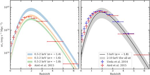
Comparison of the X-ray emissivity obtained from X-ray luminosity functions and predicted by our parametric SED formulation as described in Section 3.1. The left-hand panel shows soft X-ray emissivity (0.5–2 keV range) and the right-hand panel shows hard X-ray emissivity (2–10 keV range). The emissivities obtained from our parametric approach are shown with colored shaded regions. The data points are obtained from the X-ray luminosity functions given in Ueda et al. (2014) and Aird et al. (2015) using their LDDE models. Vertical error-bars denote the range in emissivity calculated by setting the minimum luminosity in the range of |$L_{\nu _0}^{\rm min}= 0.01 - 0.1 L_{\nu _0}^*$|. Horizontal error-bars demarcate the redshift bin of the luminosity function. In soft X-ray regime our emissivity depends on the choice of α, therefore we show predictions for three values of α. At |$z$| < 1, measurements are consistent with α = −1.4, while at |$z$| > 1 they are more in line with α < −1.6. For hard X-ray regime our emissivity is independent of choice of α and at |$z$| < 1 our predictions are systematically lower than the measurements. In both cases, our model predictions follow measured redshift evolution of X-ray emissivity reasonably well.
The left-hand panel of Fig. B1 shows soft X-ray emissivity along with our predictions for different values of α where shaded regions enclose the relevant energy range of 0.5−2 keV. At these energies our predictions depend on the choice of α. At |$z$| < 1 the measurements are consistent with α = −1.4 and higher than the predictions for α < −1.4, whereas at |$z$| > 1 they are more in line with α < −1.6. The right-hand panel of Fig. B1 shows hard X-ray emissivity along with our prediction for α = −1.8 for relevant energy range of 2−10 keV. At these energies our predictions are independent of the choice of α. At |$z$| < 1 our predictions are systematically lower than the measurements but consistent at higher-|$z$|. Nevertheless, the redshift evolution of the emissivities in both soft and hard X-ray regime is reproduced quite well by our models. Note that our parametric SED does not evolve with redshift but the normalization that is anchored with respect to type 1 QSO emissivity evolves. The reasonable agreement among our predictions and the intrinsic emissivities and their redshift evolution, along with its success to reproduce the local X-ray and γ-ray background, justify our simple parametric approach.
APPENDIX C: γ-RAY OPACITY
Using the above equation, we calculate τγ(νγ, |$z$|) at different |$z$| for our fiducial EBL model (Q18) and EBL model with α = −1.4. Note that to estimate τγ we include CMB in our EBL models. Results for three redshifts are shown in Fig. C1. The different features seen in τγ(νγ) can be naively mapped to the features seen in the EBL. For example, the γ-rays with Eγ < 20/(1 + |$z$|) GeV (0.1/(1 + |$z$|) GeV) are attenuated by EBL with Eebl > 13.6 eV (500 eV), the γ-rays with Eγ > 100/(1 + |$z$|) TeV are affected by CMB, and the bump in τγ around 100 GeV is due to rest of the EBL. The shaded region in Fig. C1 shows the observationally relevant opacities from 0.1 to 10. Within this region, EBL models with different α give same τγ since it is dominated by low-energy photons (Eebl < 10 eV) that do not depend on the value of α. Fig. C1 shows that the intrinsic SED of blazars at E > 100 GeV in our formalism (Section 3) will be severely different from the one given by equation (13). The τγ values for our fiducial EBL model are available online.5
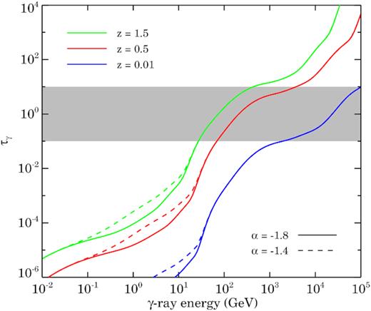
Optical depth (τγ) encountered by γ-rays for different energy (in GeV) observed on the Earth, which were emitted from redshift |$z$| = 0.01 (blue curves), |$z$| = 0.5 (red curves), and |$z$| = 1.5 (green curves). Solid and dashed curves are for our EBL models with α = −1.8 (fiducial) and α = −1.4 respectively. τγ is calculated by including CMB in both EBL models. Shaded region shows observationally relevant τγ values from 0.1 to 10, which are insensitive to the EBL photons with energy |$E\lt 10$| eV and thus on values of assumed α.
APPENDIX D: FRACTION OF TYPE 2 QSOs
In Section 3, the full SED of QSOs (kν) has been constructed to reproduce the X-ray and γ-ray background measurements. For such a constructed SED, the frequency-dependent ratio of Type-2 QSO SED and full SED, |$k^{\rm Q2}_{\nu }/k_{\nu }$|, can be interpreted as the fraction of the type 2 QSOs, which is luminosity weighted and redshift independent. This fraction is decided by our constructed SED of type 1 QSOs in the X-ray energies, which depends on the value of α. Note that we have also included blazar contribution in |$k^{\rm Q2}_{\nu }$|. In the left-hand panel of Fig. D1 we plot the ratio |$k^{\rm Q2}_{\nu }/k_{\nu }$| for different values of α (from equations 11–13). The α dependence can be easily seen in the plot. The small value of α leads to less emissivity from type 1 QSOs requiring more contribution from type 2 QSOs giving rise to the higher value of their fraction. At energies less than 1 keV (2 keV), the fraction of type 2 QSOs is less than 0.2 (0.5) for all α. At energies less than 500 eV, the contribution from type 2 QSOs drops below 5 per cent. Type 2 QSOs contribute significantly at hard X-ray energies around 10–100 keV consistent with the requirement of a large number of highly obscured type 2 QSOs in X-ray population synthesis models. At energies more than 1000 keV, the fraction of type 2 QSOs is unity owing to the fact that blazars are sole contributers at these energies (see also Draper & Ballantyne 2009). For comparison with the definition of the Compton thin and Compton thick type 2 QSOs, as the contribution to X-ray background at energies 2–10 keV and 10–30 keV, respectively, we plot a range in the fraction at these energies for different values of α in the right-hand panel of Fig. D1. We find that the fraction of Compton thin QSOs to vary between 0.2 and 0.8 for different α. It is 0.44–0.73 for our fiducial α = −1.8 model. For α ≤ −1.5, it varies from 0.38 to 0.78. These values are consistent with recent measurements (e.g. Buchner et al. 2015; Georgakakis et al. 2017; Vito et al. 2018) as well as with the prediction from X-ray population synthesis models (Treister & Urry 2006; Gilli et al. 2007). We need 20–30 per cent more contribution in 10–30 keV energy range from Compton thick QSOs, consistent with the predictions from Draper & Ballantyne (2009); however, it depends on the contribution of blazars that we do not resolve. All this interpretation is subject to our construction of type 1 QSO SED in X-rays. One can always adjust it to get different numbers while being consistent with the observed X-ray and γ-ray background. Note that our motivation is not to understand the fraction of type 2 QSOs but to provide an observationally consistent high-energy background.
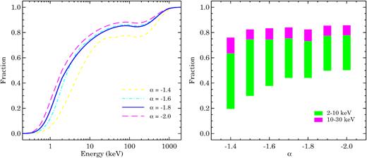
Left-hand panel: The fraction of type 2 QSOs defined as a ratio |$k^{\rm Q2}_{\nu }/k_{\nu }$| (see Section 3, equations 11–13) with energy in keV. The fraction also gives contribution of type 2 QSOs and blazars to EBL relative to type 1 QSOs for the SED templates used in our model. It depends on the extreme-UV power law index α of the type 1 QSO SED. At very high energies, fraction reaches unity due to blazar contribution included in the |$k^{\rm Q2}_{\nu }$|. Right-hand panel: The range in the fraction of type 2 QSOs in two energy ranges, 2–10 keV and 10–30 keV, for different values of α. The fraction in the energy range 2–10 keV and 10–30 keV can be thought as the fraction of type 2 QSOs that are Compton thin and Compton thick, respectively. Out of total type 2 QSOs, 20–30 per cent contribution comes from Compton thick QSOs.
APPENDIX E: EBL MODELS WITH DIFFERENT VALUES OF α
Here, we provide the EBL models (plots and tables) obtained for different values of α ranging from −1.4 (Shull et al. 2012; Stevans et al. 2014) to −2.0 (Lusso et al. 2013; Khaire 2017) in the interval of 0.1. Fig. E1 shows photoionization rates |$\Gamma _{\rm H\, {\scriptscriptstyle I}}(z)$| and |$\Gamma _{\rm He \, {\scriptscriptstyle II}}(z)$|, Fig. E2 shows photoheating rates ξH i and ξHe ii, and Tables E1 to E7 provide these values for EBL models with different α from z = 0 to 15 including for He|$\, \, {\rm {\scriptstyle I}}$|. Fig. E3 shows the local EBL from FIR to γ-rays and Fig. E4 shows UVB at redshifts |$z$| = 0–5. Refer to Section 4 for the relevant discussion on the trends seen in these plots.
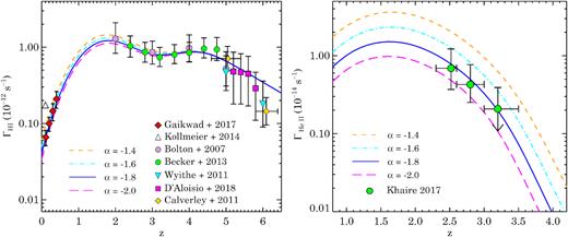
The photoionization rates of H|$\, \, {\rm {\scriptstyle I}}$| (ΓH i; left-hand panel) and He|$\, \, {\rm {\scriptstyle II}}$| (ΓHe ii; right-hand panel) with |$z$| from UVB models with different α. Various data points in the left-hand panel show the recent measurements of ΓH i. The ΓHe ii from Khaire (2017) is obtained by using the measurements of |$\tau _{\alpha }^{\rm He II}$| from Worseck et al. (2016).

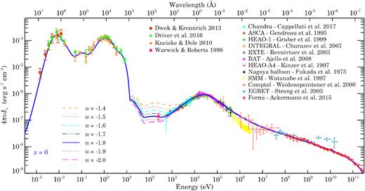
The intensity of |$z$| = 0 EBL models with different α from FIR to TeV γ-rays. For details on data points, refer to Section 4.3.
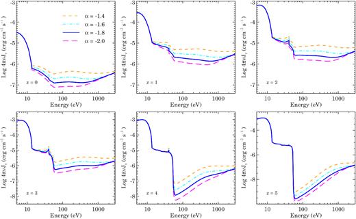
Spectrum of UVB models obtained for different values of α with energy (from 5 to 3000 eV) at |$z$| = 0, 1, 2, 3, 4, and 5. Solid blue curves show our fiducial UVB models with α = −1.8. The y-axis scales are kept same for top three panels and bottom two panels to see relative change in intensity.
Photoionization and photoheating rates for our fiducial Q18 UVB model.
| |$z$| | |$\Gamma _{\rm H \, {\scriptscriptstyle I}}$| | |$\Gamma _{\rm He \, {\scriptscriptstyle I}}$| | |$\Gamma _{\rm He \, {\scriptscriptstyle II}}$| | |$\xi _{\rm H \, {\scriptscriptstyle I}}$| | |$\xi _{\rm He \, {\scriptscriptstyle I}}$| | |$\xi _{\rm He \, {\scriptscriptstyle II}}$| |
|---|---|---|---|---|---|---|
| s−1 | s−1 | s−1 | eV s−1 | eV s−1 | eV s−1 | |
| 0.0 | 4.058e-14 | 1.869e-14 | 6.262e-16 | 1.507e-13 | 1.494e-13 | 1.248e-14 |
| 0.1 | 6.310e-14 | 3.041e-14 | 9.453e-16 | 2.381e-13 | 2.383e-13 | 1.857e-14 |
| 0.2 | 9.353e-14 | 4.695e-14 | 1.378e-15 | 3.575e-13 | 3.640e-13 | 2.670e-14 |
Photoionization and photoheating rates for Q14 UVB model.
| |$z$| | |$\Gamma _{\rm H \, {\scriptscriptstyle I}}$| | |$\Gamma _{\rm He \, {\scriptscriptstyle I}}$| | |$\Gamma _{\rm He \, {\scriptscriptstyle II}}$| | |$\xi _{\rm H \, {\scriptscriptstyle I}}$| | |$\xi _{\rm He \, {\scriptscriptstyle I}}$| | |$\xi _{\rm He \, {\scriptscriptstyle II}}$| |
|---|---|---|---|---|---|---|
| s−1 | s−1 | s−1 | eV s−1 | eV s−1 | eV s−1 | |
| 0.0 | 6.105e-14 | 3.709e-14 | 1.755e-15 | 2.544e-13 | 3.467e-13 | 3.675e-14 |
| 0.1 | 9.188e-14 | 5.816e-14 | 2.588e-15 | 3.895e-13 | 5.325e-13 | 5.372e-14 |
| 0.2 | 1.324e-13 | 8.706e-14 | 3.692e-15 | 5.691e-13 | 7.863e-13 | 7.588e-14 |
Photoionization and photoheating rates for Q15 UVB model.
| |$z$| | |$\Gamma _{\rm H \, {\scriptscriptstyle I}}$| | |$\Gamma _{\rm He \, {\scriptscriptstyle I}}$| | |$\Gamma _{\rm He \, {\scriptscriptstyle II}}$| | |$\xi _{\rm H \, {\scriptscriptstyle I}}$| | |$\xi _{\rm He \, {\scriptscriptstyle I}}$| | |$\xi _{\rm He \, {\scriptscriptstyle II}}$| |
|---|---|---|---|---|---|---|
| s−1 | s−1 | s−1 | eV s−1 | eV s−1 | eV s−1 | |
| 0.0 | 5.480e-14 | 3.099e-14 | 1.339e-15 | 2.214e-13 | 2.773e-13 | 2.745e-14 |
| 0.1 | 8.320e-14 | 4.907e-14 | 1.989e-15 | 3.418e-13 | 4.304e-13 | 4.039e-14 |
| 0.2 | 1.208e-13 | 7.403e-14 | 2.856e-15 | 5.031e-13 | 6.412e-13 | 5.741e-14 |
Photoionization and photoheating rates for Q16 UVB model.
| |$z$| | |$\Gamma _{\rm H \, {\scriptscriptstyle I}}$| | |$\Gamma _{\rm He \, {\scriptscriptstyle I}}$| | |$\Gamma _{\rm He \, {\scriptscriptstyle II}}$| | |$\xi _{\rm H \, {\scriptscriptstyle I}}$| | |$\xi _{\rm He \, {\scriptscriptstyle I}}$| | |$\xi _{\rm He \, {\scriptscriptstyle II}}$| |
|---|---|---|---|---|---|---|
| s−1 | s−1 | s−1 | eV s−1 | eV s−1 | eV s−1 | |
| 0.0 | 4.944e-14 | 2.602e-14 | 1.027e-15 | 1.938e-13 | 2.234e-13 | 2.071e-14 |
| 0.1 | 7.568e-14 | 4.162e-14 | 1.536e-15 | 3.016e-13 | 3.502e-13 | 3.064e-14 |
| 0.2 | 1.107e-13 | 6.333e-14 | 2.220e-15 | 4.472e-13 | 5.266e-13 | 4.379e-14 |
Photoionization and photoheating rates for Q17 UVB model.
| |$z$| | |$\Gamma _{\rm H \, {\scriptscriptstyle I}}$| | |$\Gamma _{\rm He \, {\scriptscriptstyle I}}$| | |$\Gamma _{\rm He \, {\scriptscriptstyle II}}$| | |$\xi _{\rm H \, {\scriptscriptstyle I}}$| | |$\xi _{\rm He \, {\scriptscriptstyle I}}$| | |$\xi _{\rm He \, {\scriptscriptstyle II}}$| |
|---|---|---|---|---|---|---|
| s−1 | s−1 | s−1 | eV s−1 | eV s−1 | eV s−1 | |
| 0.0 | 4.468e-14 | 2.194e-14 | 7.955e-16 | 1.701e-13 | 1.814e-13 | 1.586e-14 |
| 0.1 | 6.895e-14 | 3.540e-14 | 1.196e-15 | 2.670e-13 | 2.870e-13 | 2.357e-14 |
| 0.2 | 1.015e-13 | 5.425e-14 | 1.738e-15 | 3.984e-13 | 4.350e-13 | 3.382e-14 |
Photoionization and photoheating rates for Q19 UVB model.
| |$z$| | |$\Gamma _{\rm H \, {\scriptscriptstyle I}}$| | |$\Gamma _{\rm He \, {\scriptscriptstyle I}}$| | |$\Gamma _{\rm He \, {\scriptscriptstyle II}}$| | |$\xi _{\rm H \, {\scriptscriptstyle I}}$| | |$\xi _{\rm He \, {\scriptscriptstyle I}}$| | |$\xi _{\rm He \, {\scriptscriptstyle II}}$| |
|---|---|---|---|---|---|---|
| s−1 | s−1 | s−1 | eV s−1 | eV s−1 | eV s−1 | |
| 0.0 | 3.685e-14 | 1.586e-14 | 4.860e-16 | 1.332e-13 | 1.221e-13 | 9.640e-15 |
| 0.1 | 5.775e-14 | 2.604e-14 | 7.368e-16 | 2.121e-13 | 1.967e-13 | 1.439e-14 |
| 0.2 | 8.619e-14 | 4.048e-14 | 1.079e-15 | 3.205e-13 | 3.029e-13 | 2.075e-14 |
Photoionization and photoheating rates for Q20 UVB model.
| |$z$| | |$\Gamma _{\rm H \, {\scriptscriptstyle I}}$| | |$\Gamma _{\rm He \, {\scriptscriptstyle I}}$| | |$\Gamma _{\rm He \, {\scriptscriptstyle II}}$| | |$\xi _{\rm H \, {\scriptscriptstyle I}}$| | |$\xi _{\rm He \, {\scriptscriptstyle I}}$| | |$\xi _{\rm He \, {\scriptscriptstyle II}}$| |
|---|---|---|---|---|---|---|
| s−1 | s−1 | s−1 | eV s−1 | eV s−1 | eV s−1 | |
| 0.0 | 3.364e-14 | 1.361e-14 | 3.860e-16 | 1.187e-13 | 1.015e-13 | 7.721e-15 |
| 0.1 | 5.309e-14 | 2.250e-14 | 5.867e-16 | 1.903e-13 | 1.649e-13 | 1.152e-14 |
| 0.2 | 7.974e-14 | 3.519e-14 | 8.619e-16 | 2.893e-13 | 2.555e-13 | 1.662e-14 |
Note: Full Tables E1–E7 in machine-readable format are available to download at http://www.iucaa.in/projects/cobra/ and at http://vikramkhaire.weebly.com/downloads.html .
