


ABSTRACT
The extended Baryon Oscillation Spectroscopic Survey (eBOSS) is one of the first of a new generation of galaxy redshift surveys that will cover a large range in redshift with sufficient resolution to measure the baryon acoustic oscillations signal. For surveys covering a large redshift range we can no longer ignore cosmological evolution, meaning that either the redshift shells analysed have to be significantly narrower than the survey, or we have to allow for the averaging over evolving quantities. Both of these have the potential to remove signal: analysing small volumes increases the size of the Fourier window function, reducing the large-scale information, while averaging over evolving quantities can, if not performed carefully, remove differential information. It will be important to measure cosmological evolution from these surveys to explore and discriminate between models. We apply a method to optimally extract this differential information to mock catalogues designed to mimic the eBOSS quasar sample. By applying a set of weights to extract redshift-space distortion measurements as a function of redshift, we demonstrate an analysis that does not invoke the problems discussed above. We show that our estimator gives unbiased constraints.
1 INTRODUCTION
The extended Baryon Oscillation Spectroscopic Survey (eBOSS; Dawson et al. 2016; Zhao et al. 2016; Blanton et al. 2017), which commenced in 2014 July, will cover the largest volume to date of any cosmological redshift survey with a density sufficient to extract useful cosmological information. eBOSS observations will target multiple density-field tracers, including more than |$250\, 000$| luminous red galaxies (LRGs), |$195\, 000$| emission line galaxies (ELGs) at effective redshifts |$z$| = 0.72 and 0.87 and over |$500\, 000$| quasars in the range 0.8 < |$z$| < 2.2. The survey’s goals include the distance measurement at |$1\hbox{--}2{{\, \rm per\, cent}}$| accuracy with the baryon acoustic oscillations (BAO) peak on the LRG sample and the first BAO measurements using quasars as density tracers over the redshift range 1 < |$z$| < 2 (the first clustering measurements were recently presented in Ata et al. 2018). The wide redshift range covered compared with that in previous redshift surveys represents a unique opportunity to test and discriminate between different cosmological scenarios on the basis of their evolution in redshift. Full survey details can be found in Dawson et al. (2016).
The clustering analysis strategy adopted for most recent galaxy survey analyses was based on computing the correlation function or the power spectrum for individual samples or subsamples, over which the parameters being measured were assumed to be unvarying with redshift. The measurements were then considered to have been made at an effective redshift (see e.g. Anderson et al. 2014; Alam et al. 2017). In particular, Alam et al. (2017) divided the full the Baryon Oscillation Spectroscopic Survey (BOSS) volume in three overlapping redshift bins and repeated the measurement in each subvolume. This technique has many disadvantages: the choice of bins is a balance between having enough data for a significant detection in each bin leading to Gaussian errors and having bins small enough that there is no cosmological evolution across them, leading to a degrading compromise. The technique also ignores information from the cross-correlation between galaxies in different redshift bins, potentially ignoring signal. Sharp cuts in redshift will also introduce ringing artefacts in the Fourier space, potentially causing complications in the analysis.
To complicate analyses further, many mock catalogues currently used to compare to the data intrinsically lack evolution, or ‘light-cone’ effects, being drawn from simulation snapshots. Although this is a separate problem, these differences limit the tests of the effects of evolution that can be performed, and have the potential to hide biases caused by evolution.
Recent work by Zhu, Padmanabhan & White (2015), Ruggeri et al. (2017), and Mueller, Percival & Ruggeri (2018) introduced an alternative approach to the redshift binning. The idea is to consider the whole volume of the survey and optimally compress the information in the redshift direction by applying a set of redshift weights to all galaxies, and only then computing the weighted correlation function. Comparing measurements made using different sets of redshift weights maintains the sensitivity to the underlying evolving theory. The sets of weights are derived in order to minimize the error on the parameters of interest. In addition, by applying the redshift weighting technique instead of splitting the survey, is it possible to compute the correlation function to larger scales whilst accounting for the evolution in redshift; this was particularly clear in Mueller et al. (2018), which considered this method to optimize the measurement of local primordial non-Gaussianity, which relies on large scales. Further, Zhu et al. (2016) showed that the application of a weighting scheme rather than splitting into bins also improves BAO measurements.
The need to correctly deal with evolution will increase for the Dark Energy Spectroscopic Instrument (DESI) and Euclid experiments, which will cover a broad redshift range and have significantly reduced statistical measurement errors compared to current surveys in any particular redshift range. The DESI1 is a new multi-object spectrograph (MOS) currently under construction for the 4-m Mayall Telescope on Kitt Peak. DESI will be able to obtain 5000 simultaneous spectra, which coupled with the increased collecting area of the telescope compared with the 2.5-m Sloan telescope, means that it can create a spectroscopic survey of galaxies ∼20 times more quickly than eBOSS. In 2020 the European Space Agency (ESA) will launch the Euclid2 satellite mission. Euclid is an ESA medium class astronomy and astrophysics space mission, and will undertake a galaxy redshift survey over the redshift range 0.9 < |$z$| < 1.8, while simultaneously performing an imaging survey in both visible and near-infrared bands. The complete survey will provide hundreds of thousands images and several tens of petabytes of data. About 10 billion sources will be observed by Euclid out of which several tens of million galaxy redshifts will be measured and used to make galaxy clustering measurements.
In this work, we test the redshift weighting approach by analysing a set of 1000 mocks catalogues (Chuang et al. 2015) designed to match the eBOSS quasar sample. This quasar sample has a low density (|$82.6\, \rm objects\, deg^{-2}$|) compared to that of recent galaxy samples, and covers a total area over 7500 |$\rm deg^2$|. The quasars are highly biased targets and we expect their bias to evolve with redshift, b(|$z$|) ∝ c1 + c2(1 + |$z$|)2, with constant values c1 = 0.607 ± 0.257, c2 = 0.274 ± 0.035, as measured in Laurent et al. (2017).
Although the mocks are not drawn from N-body simulations, they have been calibrated to match one of the BigMultiDark (BigMD; Klypin et al. 2016), a high-resolution N-body simulation, with 38403 particles covering a volume of |$(2500\, h^{-1}\, \text{Mpc})^3$|. The BigMD simulations were performed using gadget-2 (Springel 2005), with Λ cold dark matter (ΛCDM) Planck cosmological constraints as a fiducial cosmology. Ωm = 0.307, Ωb = 0.048206, σ8 = 0.8288, ns = 0.96, |$H_0 = 100\, h\, \rm km\, s^{-1}\, \rm Mpc^{-1}$|, and h = 0.6777. In Chuang et al. (2015) the authors showed that effective Zel’dovich approximation mocks (EZmocks) are nearly indistinguishable from the full N-body solutions: they reproduce the power spectrum within |$1{{\, \rm per\, cent}}$|, up to |$k = 0.65\, h\, \rm Mpc^{-1}$|. The mocks are created using a new efficient methodology based on the effective Zel’dovich approximation approach including stochastic scale-dependent, non-local, and non-linear biasing contribution. The EZmocks used for the current analysis are the light-cone catalogues, realized on seven different snapshots at |$z$| = 0.9, 1.1, 1.3, 1.5, 1.6, 1.7, and 2.0. The full simulations incorporate the redshift evolution for f, σ8, the BAO damping, and the non-linear density and velocity effects.
In a companion paper (Ruggeri et al. 2017), we will apply the weighting scheme to measure redshift-space distortions (RSDs) from the eBOSS Data Release 14 (DR14) quasar data. In this paper, we validate the procedure and test for optimality. By fitting to the evolution with a model for bias and cosmology, we are able to fit simultaneously the evolution of the growth rate f(|$z$|), the amplitude of the dark matter density fluctuations σ8(|$z$|), and the galaxy bias b(|$z$|); breaking part of the degeneracy inherent in standard measurements of fσ8 and bσ8 when only one effective redshift is considered. We show that the redshift weighting scheme gives unbiased measurements.
The weights can be applied in both configuration and Fourier space. In this paper, we focus on Fourier space, as there is some evidence that this provides stronger RSDs constrains, given the current scale limits within which the clustering can be modelled to a reasonable accuracy (Alam et al. 2017). In addition, the calculation of the power spectrum moments is significantly faster than the correlation function (Bianchi et al. 2015; Scoccimarro 2015). Working in Fourier space requires a reformulation of the window selection to account for an evolving power spectrum.
The paper is organized as follows. Section 2 reviews the derivation of optimal weights, presenting two schemes that differ in the cosmological model to be tested. In Section 3, we review the redshift-space power spectrum model at a single redshift; In Section 4, we model the power spectrum and the window function to obtain the redshift evolving power spectrum. In Section 5, we present the result of our analysis.
2 OPTIMAL WEIGHTS
We make use of two different sets of weights. The first explores deviations from the ΛCDM model by altering the evolution of Ωm in redshift. This model ties together growth and geometry, but can also be used after fixing the expansion rate to match the prediction of the ΛCDM model. The second parametrizes the fσ8 parameter combination measured by RSD, allowing for a more standard test of deviations from ΛCDM. Here, the growth and geometry are artificially kept separate as fσ8 only affects cosmological growth. In both cases the weights are computed selecting a flat ΛCDM scenario as fiducial model. Note that, as discussed in Ruggeri et al. (2017) and Zhu et al. (2015), the choice of an inaccurate fiducial model for the weights would only affect the variance of the quantities constrained and not the best-fitting values.
Note that the weights as they are reported in equation (1) aim to compress different measurements of the power spectrum across a range of different redshifts. In fact, we apply weights to each galaxy in order to avoid binning, by assuming the relation |$w_{\text{gal}} = \sqrt{w_P}$|, with |$w$|P denoting the weights defined in equation (1), which relies on the scale dependence of the weights being smooth on the scale of interests for clustering.
2.1 Optimal weights for Ωm
The choice of parametrizing Ωm (and hence the Hubble parameter, the angular diameter distance, and the growth rate) in terms of q0, q1, and q2 allows us to simultaneously investigate small deviations using a common framework: e.g. departures from a fiducial cosmology and geometry are accounted through the fiducial Hubble constant and angular diameter distance H(Ωm), DA(Ωm); further, modified gravity models can be accounted through the growth rate, f(Ωm).
Fig. 1 shows an example of the weights as derived in Ruggeri et al. (2017) that optimize the measurements of the qi parameters in a ΛCDM fiducial background for a redshift-space power spectrum. Since each multipole contains information about Ωm(|$z$|), our set of weights is derived to be optimal for the first two non-null moments of the power spectrum on the Legendre polynomial basis for each qi parameter. Continuous lines indicate the weights for the monopole with respect to q0 (red line) and q1 (orange line); dashed lines indicate the weights for the quadrupole with respect q0, q1 (red and orange lines). All the weights are normalized to be equal 1 at the pivot redshift.
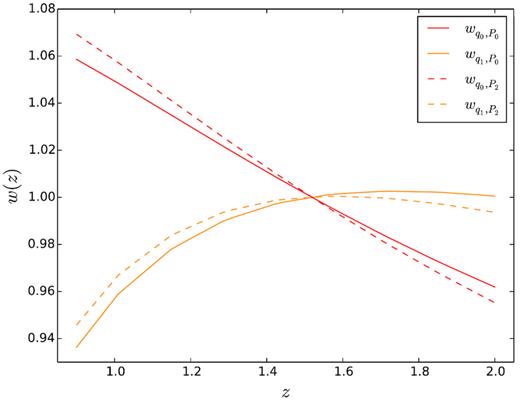
The weights for the monopole and quadrupole with respect to the qi parameters.
2.2 Optimal weights for |$\boldsymbol {f \sigma _8}$|
A strong effect on the set of weights is caused by the assumptions we make for galaxy bias. If we set the bias as an unknown parameter, and we marginalize over it, then we cannot deduce any information about structure growth from the amplitude of the density power spectrum. Marginalizing over the bias will not affect the other parameters provided that the bias model is correct. We do not have a sufficiently accurate model of galaxy formation and evolution that the bias can be accurately predicted. As explained in Section 4.3, in this work, we describe it using free functions and making sure there is enough freedom in other parameters.
This is the case for the expansion around [fσ8], where we considered [bσ8] and [fσ8] as independent parameters. However, if we constrain b(|$z$|) to match a fiducial model, we will derive weights that make use of the information coming from the amplitude of the power spectrum. For the expansion around Ωm, we can choose whether or not to include this information.
3 MODELLING THE ANISOTROPIC GALAXY POWER SPECTRUM AT A SINGLE REDSHIFT
4 MODELLING THE EVOLVING GALAXY POWER SPECTRUM
4.1 Redshift weighted multipoles without window function
In general when estimating the power spectrum of a three-dimensional redshift survey that measured is the underlying power spectrum convolved with the window function. Therefore to compare the model with the data we first convolve it with the window determined by the survey geometry. In the next section, we derive a general relation between the measured P and the window function to extend the treatment of Feldman et al. (1994), (equation 2.1.4) to the case where the power spectrum is evolving with redshift.
4.2 Redshift weighted multipoles including the survey window effect
We study the window function for the evolving power spectrum using a generalized Hankel transformation between power spectrum and correlation function moments, where the window applied is also decomposed into a set of multipoles. This is an extension of the work by Wilson et al. (2017) and Beutler et al. (2017), which presented a method to convolve model power spectra with the window function for a non-evolving power spectrum. We consider the case where the underlying correlation function ξ is dependent on both the separation r = |ri − rj| (with ri and rj position of galaxies of each pair) and the mean redshift of each galaxy pair ξ[ri(|$z$|i), |ri − rj|]. Here we have assumed that cosmological evolution is negligible over the range of redshifts covered by every pair, so we can quantify the clustering of each using the correlation function at the mean redshift.
Note that when computing the mask |$W (\boldsymbol {x})$| using the random catalogue we include the redshift weights, in the same way the standard FKP weights have been included in traditional analyses (e.g. Beutler et al. 2017).
4.3 Bias evolution
The evolution in redshift of the galaxy bias, b(|$z$|), strongly depends on the targets considered. In Ruggeri et al. (2017) we compared the weights for different b(|$z$|) relations and showed that the weights are not significantly sensitive to the different b(|$z$|) considered.
5 FITTING TO THE MOCK DATA
5.1 Power spectrum measurement
To compute the power spectrum moments with respect to the LOS, we make use of the estimator introduced in Bianchi et al. (2015). This FT-based algorithm uses multiple FTs to track the multipole moments, in the local plane-parallel approximation where we have a single LOS for each pair of galaxies. This estimator has been already used in recent analysis (Beutler et al. 2017) that confirmed the advantages of using such decomposition: it reduces the computational time from N2 associated to naive pair counting analysis (Yamamoto et al. 2006) to ∼Nlog N.
Redshift weights are included in the estimator, by defining the weighted galaxy number density as |$n_\text{g} (\boldsymbol {r}) w$|. As discussed in Section 2, we have derived the galaxy weights from the square-root of the power spectrum weights, under the assumption that the scale dependence in the weights is smooth compared to the scale of interest for our clustering measurements.
5.2 Covariance matrix estimation
We evaluate the covariance matrix for the data vector Π using 1000 EZmocks described in Section 1. Differences between mocks arise because of sample variance – we probe different patches of the Universe, and shot noise – we sample the density field with different galaxies. These are the primary sources of error in clustering measurements.
Note that when inverting the covariance matrix we include the Hartlap factor (Hartlap, Simon & Schneider 2007) to account for the fact that |$\boldsymbol{\sf{C}}$| is inferred from mock catalogues. The choice of nb = 10 given NT = 1000 mocks available ensures that the covariance matrix is positive definite.
5.3 Maximizing the likelihood
In this analysis we limit ourselves to linear order deviations about our fiducial ΛCDM model, for both fσ8(|$z$|) and Ωm(|$z$|) described in Sections 2.1 and 2.2, since the data cannot capture second-order deviations. We discuss this further in Section 7.
6 MEASURING RSD WITH THE EVOLVING GALAXY POWER SPECTRUM
The fits presented in this section are performed using a Markov chain Monte Carlo (MCMC) code, implemented to efficiently account for the degeneracies between the parameters; in all the fit performed we select a range between k = 0.01 and |$0.2\, h \, \rm Mpc^{-1}$|. For each scenario explored we run 10 independent chains, satisfying the Gelman–Rubin convergence criteria (Gelman & Rubin 1992) with the requirement of R − 1 < 104, where R corresponds to the ratio between the variance of chain mean and the mean of chain variances. All the results presented are obtained after marginalizing on the full set of parameters, including the nuisance parameters (shot noise and velocity dispersion). All the contour plots are produced using the public GetDist libraries.3
We fit the weighted monopole and quadrupole computed on a subset of 20 EZmocks, for both the Ωm and the fσ8-optimized weights, while keeping the distance–redshift relation fixed to the fiducial cosmology, i.e. α∥ = α⊥ = 1.
We do not consider the full set of 1000 EZmocks for the following reasons: first, we are limited by the EZmocks accuracy in describing non-linearities in galaxy bias and velocities; further by the accuracy in the light-cone describing the redshift evolution for fσ8 that is included as a step function. Thus we do not believe that the mocks support us looking at deviations from the model at better accuracy than this. However, the error on our constraints is still |$1/\sqrt{20}$| smaller than what we expect on the eBOSS quasars constraints. The analysis has been performed on different subset of 20 mocks out of the 1000 available to verify that the outcomes do not depend on a particular subsample choice.
Our analysis is presented as follow. In Section 6.1, we present the result obtained with the Ωmweights fitting for q0, q1, bσ8(|$z$|p), |${\partial} b \sigma _8/{\partial} z|_{z_\text{p}}$|, b2, σ|$v$|, and shot noise S. In parallel we present the fit for p0, p1, bσ8(|$z$|p), |${\partial} b \sigma _8/{\partial} z|_{z_\text{p}}$|, b2, and σ|$v$| when applying the fσ8 weights.
In Section 6.2, we investigate the impact of the bias assumption on the constraints, showing a comparison between bias evolving and constant with redshift.
In Section 6.3, we compare the results obtained with the redshift weights approach with the analysis performed considering one constant redshift slice, i.e. considering all the parameters (fσ8, bσ8, σ|$v$|, b2, S) in the power spectra at their value at the pivot redshift |$z$| = 1.55 and applying FKP weights only (for simplicity of the notation from now on we refer to this as traditional analysis).
Differently from Zhu et al. (2016), we compare the redshift weights analysis with the standard analysis used for previous RSD measurements (see e.g. Beutler et al. (2017)) rather than testing the weights |$w$|q, i, |$w$|p, i = 1. The main focus of this work is to test that our analysis is not biased by introducing evolution in the power spectrum and in the window function. We rely on the Fisher matrix theory correctly selecting the set of weights optimal with respect to the qi, pi errors.
6.1 Redshift weights fit
Fig. 2 shows the posterior likelihood distributions from the analysis performed with the set of redshift weights optimized to constrain Ωm(|$z$|) (blue contour plots), using the monopole and the quadrupole; we fit for q0, q1 that describe up to linear order deviations in the evolution of Ωm(|$z$|) according to |$\Lambda \rm CDM$| model; we also vary the galaxy bias parameters modelled as in Section 4.3, while we fix the second-order non-local bias, bs2, and third-order non-local bias, b3nl, terms as shown in equation (35). To summarize we fit for seven parameters: q0, q1, bσ8(|$z$|p), |${\partial} b \sigma _8 /{\partial} z|_{z_\text{p}}$|, b2σ8(|$z$|p), σ|$v$|, and shot noise S.
![Likelihood distributions for the analysis of the average of 20 EZmocks. We show the results for q0, q1, bσ8($z$p), ${\partial} b\sigma _8/{\partial} z$, marginalized over the full set parameters (including b2σ8($z$p), σ$v$, S not displayed here). We multifit two weighted monopoles and two weighted quadrupoles [one for each weight function ($w_{0,p_i}$, $w_{2,p_i}$)]. The fitting range is $k = 0.01\hbox{--}0.2\, h\, \rm Mpc^{-1}$ for both the monopole and quadrupole.](https://oup.silverchair-cdn.com/oup/backfile/Content_public/Journal/mnras/484/3/10.1093_mnras_sty3452/1/m_sty3452fig2.jpeg?Expires=1750223158&Signature=qME~JpKyBTFtIILyJg34YjYLo~DVSxoByDAKFTkmQOcwwmTCAg75EyQcCyJUebadnTI4ebgEvPw6O-egzaj8QDHd36YO8ODxdGeXed7sVy1i29hoX8A-RLtChkg73HmNIgN796V3Yp5pcIBT3DjBplEs9BgwMBHsAslar91Yc-ATjM4axD2r45AD6P77w45rP9akbW~DoNP3NrsxRIjtw8M4HfSmIk5IFht4Glz0FFuHLvsX2mxe2Z66u9F0J6HhS9cWLlyYsaBo5suNb5HL-3iSGLUVeSahWJjfBP7mExr0~9VhkKwufTPuzc0c29npfRXoDQ91Xlj~dJZa39QZMw__&Key-Pair-Id=APKAIE5G5CRDK6RD3PGA)
Likelihood distributions for the analysis of the average of 20 EZmocks. We show the results for q0, q1, bσ8(|$z$|p), |${\partial} b\sigma _8/{\partial} z$|, marginalized over the full set parameters (including b2σ8(|$z$|p), σ|$v$|, S not displayed here). We multifit two weighted monopoles and two weighted quadrupoles [one for each weight function (|$w_{0,p_i}$|, |$w_{2,p_i}$|)]. The fitting range is |$k = 0.01\hbox{--}0.2\, h\, \rm Mpc^{-1}$| for both the monopole and quadrupole.
Fig. 3 presents the results of the analysis while using the set of redshift weights optimized to constrain fσ8(|$z$|), as introduced in Section 2.2; the structure is the same as in Fig. 2. We fit for p0, p1 to constrain fσ8(|$z$|) deviations about the fiducial fσ8(|$z$|) according to |$\Lambda \rm CDM$|; we also fit for bσ8(|$z$|p), |${\partial} b \sigma _8(z) /{\partial} z$|, b2σ8(|$z$|p), σ|$v$|, and S, seven parameters in total as for the other set of weights.
![Likelihood distributions for the analysis of the average of 20 EZmocks. We show the results for p0, p1, bσ8($z$p), ${\partial} b\sigma _8/{\partial} z$, marginalized on the full set parameters (including b2σ8($z$p), σ$v$, S not displayed here). We multifit two weighted monopoles and two weighted quadrupoles [one for each weight function ($w_{0,p_i}$, $w_{2,p_i}$)]. The fitting range is $k = 0.01\hbox{--}0.2\, h\, \rm Mpc^{-1}$ for both the monopole and quadrupole.](https://oup.silverchair-cdn.com/oup/backfile/Content_public/Journal/mnras/484/3/10.1093_mnras_sty3452/1/m_sty3452fig3.jpeg?Expires=1750223158&Signature=wxen8zM-VxOEjkz-sxWPq3r3iUpVQnPoj8yxRDKoRiEi8AsPVrXM48mjpMOD3Rs6SmG233sShqNllc3c8d~A6VW2tEqZSVhbit3Pm7u-KjbmTOmfu9I3U~-saBeV6xi2HuufW73ERINyicNIW8CNQi9jpkvvY6Jzy1yypZ-rAoXJ7LMoGwY6zoVc~kFGn~wNzuSoH0ygBu16UoxBKGmGpkVCbxNZJenbB4HkzZ823ZkADVpKGNHPZboTDB3SAqzUOEXat~X-qUQSHAoU5B8XvYXywN2ZAbbQzKQoC79BdLuogPZ9FsEsAShAT1yxOlPQgEGkaRYG75c88Mgti0tgag__&Key-Pair-Id=APKAIE5G5CRDK6RD3PGA)
Likelihood distributions for the analysis of the average of 20 EZmocks. We show the results for p0, p1, bσ8(|$z$|p), |${\partial} b\sigma _8/{\partial} z$|, marginalized on the full set parameters (including b2σ8(|$z$|p), σ|$v$|, S not displayed here). We multifit two weighted monopoles and two weighted quadrupoles [one for each weight function (|$w_{0,p_i}$|, |$w_{2,p_i}$|)]. The fitting range is |$k = 0.01\hbox{--}0.2\, h\, \rm Mpc^{-1}$| for both the monopole and quadrupole.
We obtained the covariance and correlation matrix for the full set of parameters of the MCMC chains using GetDist libraries. The resulting posteriors in both Figs 2 and 3 show a correlation between the zero-order parameters, q0 (p0) and bσ8(|$z$|piv), of magnitude of ∼0.5. We also detect a relevant anticorrelation ∼− 0.4 between the slope parameter q1 (p1) and the gradient |${\partial} b \sigma _8(z) /{\partial} z$|. These non-zero correlations lead to a mild dependency between the assumed bias model (linear and non-linear in k and in |$z$|) and the slope parameter q1 (p1) without however affecting (within ∼1σ) the constraints on fσ8. In Section 6.2, we illustrate the impact of the bias evolution on the growth rate in more details. Because of the stepwise implementation of the growth rate and bias model in the mocks, the fiducial values of q0, q1 (p0, p1) are not well defined. Therefore, we do not display an expected value for pi and qi as those cannot be inferred from the fσ8 evolution included as a non-smooth step function in the mocks. However, within 1σ–2σ we recover the smooth |$\Lambda \rm CDM$| expectation values of q0 = 1 and q1 = 0.
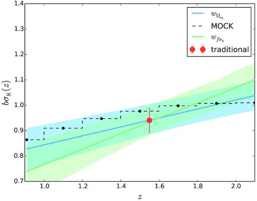
Fig. 4 shows the redshift evolution reconstructed from p0, p1 (green shaded regions) compared with the evolution reconstructed from the q0, q1 (blue shaded regions). The red point indicates the constraints at one single redshift (traditional analysis, with |$z$| = 1.55) for fσ8. We overplot the evolution of fσ8(|$z$|) as accounted in the mock light-cone (black dashed line). The plot shows that the fσ8 evolution obtained for both the Ωm and fσ8 weighting schemes is fully consistent with the cosmology contained in the mock and in full agreement with the constraints coming from the traditional analysis. For both parametrizations the errors obtained at the pivot redshift are comparable with the error we get from the traditional analysis. Note that the error from redshift weighting analysis comes from the marginalization over a set of seven parameters in contrast to the traditional analysis limited to only five free parameters.
![The reconstructed evolution of fσ8 and $68{{\, \rm per\, cent}}$ confidence level regions using the average of 20 mocks; blue shaded region shows the constraint on the evolution of fσ8 obtained by the fit of Ωm($z$, qi) using the $w_{\Omega _{\rm m}}$ optimal weights and deriving at each redshift f[Ωm($z$, qi)] times σ8[Ωm($z$, qi)]; green shaded region shows the resulting evolution when fitting for fσ8($z$, pi) at each redshift. The red point indicates the results obtained when performing the traditional analysis, with $z$piv = 1.55.](https://oup.silverchair-cdn.com/oup/backfile/Content_public/Journal/mnras/484/3/10.1093_mnras_sty3452/1/m_sty3452fig4.jpeg?Expires=1750223158&Signature=meouxQ6UKhpBqiZ6IuWisu0n49UBXOGRBUaPRYqd0~gCF3ZrEwb4BTUAEwA1znscKXtEtM-cHD1MAYnRHc89mUmLxlI~NYtYO9G9qL1cMvlchUeicGlHm6C83hqFzyQgn6s4PecgsDW4Q2T4elP58ebh8N-lqa6fBOnzUdgtl4olAmKW5nnC0x4FXpwjqvWVKkz9bejfL5PGig4G1By-vsizsoGxfAQnzXzUHu8SxXvifWy7zaHRSqcXWh2AWoCQPkKMlVTHe5M7gqhYYb7tbsKnAm8Cfyb6vFoXqQV~hnzsEiIJ4mC5MO7~fj02b2aARpeN34ZX6XToDnkf2~R4fQ__&Key-Pair-Id=APKAIE5G5CRDK6RD3PGA)
The reconstructed evolution of fσ8 and |$68{{\, \rm per\, cent}}$| confidence level regions using the average of 20 mocks; blue shaded region shows the constraint on the evolution of fσ8 obtained by the fit of Ωm(|$z$|, qi) using the |$w_{\Omega _{\rm m}}$| optimal weights and deriving at each redshift f[Ωm(|$z$|, qi)] times σ8[Ωm(|$z$|, qi)]; green shaded region shows the resulting evolution when fitting for fσ8(|$z$|, pi) at each redshift. The red point indicates the results obtained when performing the traditional analysis, with |$z$|piv = 1.55.
Away from the pivot redshift, the errors become larger for both parametrizations. At these redshifts, the major contribution to the error comes from the slope constraints (q1, p1) and the signal-to-noise ratio (S/N) is lowered due to the low number density n(|$z$|) (Ata et al. 2018). The number of quasars observed as a function of redshift also helps to explain the differences in the error as a function of redshift, with a larger error found where there are fewer quasars.
For both parametrizations, the slope parameters are degenerate with the non-linear bias parameters.
In Section 6.1, we modelled the bias evolution with a Taylor expansion up to linear order about the pivot redshift (see equation 4.3). Fig. 5 shows the bσ8(|$z$|) evolution measured using the Ωm and fσ8 weighting schemes (blue and green shaded regions). We reconstruct bσ8(|$z$|) at the different redshifts from the fit of bσ8(|$z$|p) and |${\partial} b \sigma _8(z) /{\partial} z$|. We overplot the evolution of bσ8(|$z$|) as included in the mocks (black dashed line). The red point indicates the constraints obtained by using the traditional analysis; we find full agreement at the pivot redshift between the three different analysis and within 1σ of the value included in the mocks. The bias depends significantly on redshift and in the mocks is modelled as a step function, which leads to small discrepancies with respect to both the constant and linear evolution in bσ8. We redid the fit extending the analysis to second order in bias and found consistent results but with error too large to see any improvements (high degeneracy). For the purpose of fitting eBOSS quasar sample this is more than enough and we leave for future work a more careful study of the bias effects/evolution to be performed on more accurate N-body mocks. This is discussed further in Section 7.
The reconstructed evolution for bσ8(|$z$|) and |$68{{\, \rm per\, cent}}$| confidence level regions using the average of 20 mocks; we fit the evolution for bσ8, modelled as a Taylor expansion about the pivot redshift, up to linear order. Blue shaded regions show the evolution of bσ8 through the fit of bσ8(|$z$|p), |${\partial} b \sigma _8(z) /{\partial} z$|, obtained for the Ωm(qi) analysis; green shaded regions show the analogous resulting bσ8(|$z$|) when fitting for fσ8(|$z$|, pi) at each redshift. The red point indicates the results obtained for fσ8(|$z$|piv) when performing the traditional analysis.
6.2 Constant bias versus evolving bias
We now investigate how a particular choice for the bias evolution in redshift can affect and impact the constraints on fσ8(|$z$|). To do this, we repeat the analysis as presented in Section 6.1 using the Ωm and fσ8 weights, we model Ωm(|$z$|) and fσ8(|$z$|) in the same way as in Section 6.1, but now assuming that the bias is constant with redshift, i.e. we set |${\partial} b \sigma _8(z) /{\partial} z = 0$|.
In Figs 6 and 7, we show the comparison between the results obtained with the constant bias. We display the posterior likelihood for all the quantities evaluated at the pivot redshift, fσ8(|$z$|p) bσ8(|$z$|p), σ|$v$|, b2, and S. In Fig. 6, blue contours show the likelihood distributions obtained when using the Ωm weights and considering bσ8 evolving as in equation (4.3). Dark blue contours indicate the constraints obtained when considering |${\partial} b \sigma _8(z) /{\partial} z = 0$|. In Fig. 7, we present the analogous results when using the fσ8 parametrization; green contours show the likelihood distributions obtained when using the fσ8 weights considering the bias evolving as in equation (4.3). Dark green contours correspond to the constraints obtained when we set |${\partial} b \sigma _8(z) /{\partial} z$| equal to zero.
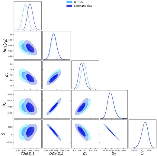
Comparison between evolving and constant bias for the Ωm-weights analysis. Blue likelihood contours indicate the constraints obtained when fitting for bσ8(|$z$|p) and |${\partial} b \sigma _8(z) /{\partial} z$|; dark blue contours indicate the constraints obtained when setting |${\partial} b \sigma _8(z) /{\partial} z = 0$| and fitting only for bσ8(|$z$|p).
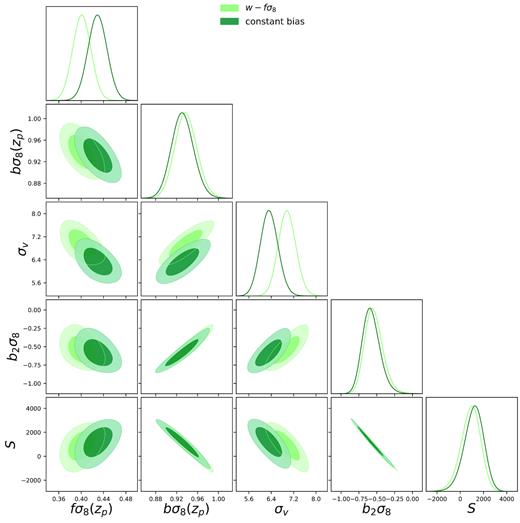
Comparison between evolving and constant bias for the fσ8-weights analysis. Green likelihood contours indicate the constraints obtained when fitting for bσ8(|$z$|p) and |${\partial} b \sigma _8(z) /{\partial} z$|; dark green contours indicate the constraints obtained when setting |${\partial} b \sigma _8(z) /{\partial} z = 0$| and fitting only for bσ8(|$z$|p).
The results obtained from the different models are consistent, but, whereas the constraints for bσ8(|$z$|p) remain unchanged, there is an evident impact on the fσ8 constraints at the pivot redshift. Forcing the bias to be constant with redshift lead to a higher value for fσ8.
This should be more important for future surveys, for which higher precision is expected: for these surveys, a careful study/treatment of the bias will be required. One approach would be to have free functions to describe the bias (e.g. Taylor expanding cosmological quantities as in the present case), and making sure there is enough freedom in the other parameters so that the measurements are applicable to a wide range of cosmological models and targets, with few assumptions. For higher S/N and more realistic mocks it would be interesting to investigate the evolution in redshift of the non-linear bias parameters and the possible impact on fσ8. In this work all of the non-linear quantities are considered at a single redshift and our tests are limited to verify that the bias does not affect the measurement of the growth, which is adequate for the current S/N level.
6.3 Weights versus no weights
We compare the analysis performed using the redshift weights approach, as presented in Section 6.1 with the traditional analysis at one constant redshift.
The traditional analysis makes use of the power spectrum moments, modelled as in Section 3, to constrain fσ8 and bσ8 at one single epoch that corresponds to the effective redshift of the survey (|$z$| = 1.55). We do the comparison for both the Ωmfσ8 weighting schemes.
Fig. 8 shows the comparison between the redshift weights analysis for Ωm (blue contours), fσ8 (green contours), and the constant redshift analysis (brown contours). In order to make the comparison between the three different analysis, we infer from the MCMC chains of qi and pi, the fσ8[|$z$|, Ωm(qi)], and fσ8(|$z$|, pi) valued at the pivot redshifts. We then compare those values with the fσ8(|$z$|p), bσ8(|$z$|p) as obtained from the traditional analysis. The last two panels in Fig. 8 show that we recover the same value for b2 and S where the evolution in redshift is not considered in all the three different analysis; the other constraints on fσ8, bσ8, and σ|$v$| are fully consistent within ∼1σ.
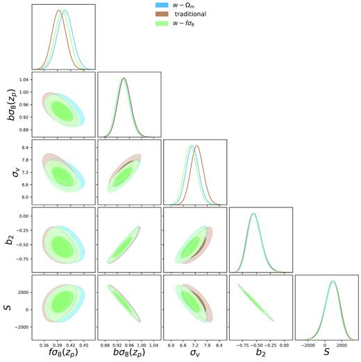
Comparison between the redshift weights analysis and the traditional analysis. Likelihood contours for fσ8, bσ8, σ|$v$|b2, and S quantities, at their pivot redshift values. Blue likelihood contours show the results obtained with the Ωm(qi) analysis; green contours show the results from the fσ8(pi) analysis; brown contours indicate the results obtained with the traditional analysis.
7 CONCLUSION
In this work we present a new approach to measure RSDs when dealing with surveys covering a wide redshift range; the redshift weights, applied to each galaxy within the sample, act as a smooth window on the data, allowing us to compress the information in the redshift direction without loss of information. In this analysis we applied the redshift weighting technique to investigate small deviation from the ΛCDM framework; we selected two different parametrization, allowing for deviation in the matter energy density and the growth rate evolution. We derived multiple sets of weights to optimize each order of those deviations. We extended the window function derivation in order to account for the redshift evolution of the power spectrum.
We compared the results obtained for the different parameters with the traditional analysis, i.e. the analysis performed considering the clustering as constant in the whole volume. We found that the redshift weights technique gives unbiased constraints for the whole redshift range, in full agreement with the traditional analysis performed at the effective redshift.
The constraints obtained fully validate the analysis (Ruggeri et al. 2018) to measure RSD on the eBOSS quasars sample where the error expected on fσ8 is about |$5{{\, \rm per\, cent}}$|. To apply the same pipeline to future surveys aiming at |${{\, \rm per\, cent}}$| level accuracy further work will be required; first, we will need to consider quadratic deviations in the evolution for both the qi and the galaxy bias parameters. In this work we only accounted for those deviations to test the robustness of the fits whereas the signal expected from the quasars sample will not be able to constrain the quadratic evolution.
Another important and interesting aspect would be to account for the AP parameters and their evolution in redshift. To perform such analysis, a set of N-body simulations that accurately describe non-linearities/light-cone evolution is also required, to reduce the degeneracies and provide a lower statistical error. We here only considered the growth alone, with better data we would be able to include both AP and growth. For the eBOSS sample, the constraints are too weak to consider this.
ACKNOWLEDGEMENTS
Ruggero Ruggeri thanks Dr Valeria Pala, and Dr Gavino Pala for all the support provided. RR and WJP acknowledge support from the European Research Council through the Darksurvey grant 614030, from the UK Science and Technology Facilities Council grant ST/N000668/1, WJP also acknowledge the UK Space Agency grant ST/N00180X/1.
Funding for SDSS-III and SDSS-IV has been provided by the Alfred P. Sloan Foundation and Participating Institutions. Additional funding for SDSS-III comes from the National Science Foundation and the US Department of Energy Office of Science. Further information about both projects is available at www.sdss.org. SDSS is managed by the Astrophysical Research Consortium for the Participating Institutions in both collaborations. In SDSS-III these include the University of Arizona, the Brazilian Participation Group, Brookhaven National Laboratory, Carnegie Mellon University, University of Florida, the French Participation Group, the German Participation Group, Harvard University, the Instituto de Astrofisica de Canarias, the Michigan State/Notre Dame/JINA Participation Group, Johns Hopkins University, Lawrence Berkeley National Laboratory, Max Planck Institute for Astrophysics, Max Planck Institute for Extraterrestrial Physics, New Mexico State University, New York University, Ohio State University, Pennsylvania State University, University of Portsmouth, Princeton University, the Spanish Participation Group, University of Tokyo, University of Utah, Vanderbilt University, University of Virginia, University of Washington, and Yale University. The Participating Institutions in SDSS-IV are Carnegie Mellon University, Colorado University, Boulder, Harvard-Smithsonian Center for Astrophysics Participation Group, Johns Hopkins University, Kavli Institute for the Physics and Mathematics of the Universe, Max-Planck-Institut für Astrophysik (MPA Garching), Max-Planck-Institut für extraterrestrische Physik (MPE), Max-Planck-Institut für Astronomie (MPIA Heidelberg), National Astronomical Observatories of China, New Mexico State University, New York University, The Ohio State University, Penn State University, Shanghai Astronomical Observatory, United Kingdom Participation Group, University of Portsmouth, University of Utah, University of Wisconsin, and Yale University. This work made use of the facilities and staff of the UK Sciama High Performance Computing cluster supported by the ICG, SEPNet, and the University of Portsmouth. This research used resources of the National Energy Research Scientific Computing Center, a DOE Office of Science User Facility supported by the Office of Science of the US Department of Energy under Contract No. DE-AC02-05CH11231.
