


Abstract
Based on the reformulation of the problem of galactic shape measurement, introduced by Tessore and Bridle, we develop and test new estimators which more efficiently solve what is now a statistical problem. Frequently only a single measurement is available from an observation made by telescopes, which may be distorted due to noise introduced in the measuring process. To soften these effects, we investigate a number of approaches, such as scaling, data censoring, or mixtures of estimators. We then run simulations for various set-ups which emulate real-life conditions, to determine practical suitability of all proposed estimation approaches.
1 INTRODUCTION
This paper is structured as follows, in the next section we focus on previously proposed estimation techniques to the newly formulated statistical problem. We shed light on the well-understood properties the parameters need to fulfil, and explain how they inspired the novel estimation approach listed in the upcoming section. With the completion of the method section, we elaborate on the simulation set-up used to investigate the performance of the proposed estimators, and discuss their properties in relation to the composure of the parameter values. In the fourth and final section, we give a conclusion on what our observations were, and give an indication on how the approximation methods should be optimally chosen in regard to signal-to-noise ratio (SNR) values and different parameter combinations. Additionally, we give a motivation for further research and new questions opened up by our results.
2 METHODS
As previously shown, both estimators are unbiased in the argument |$\arg \epsilon$| of the ellipticity, so the main improvement lies in the estimation of the radius of the complex parameter ε.
Definition of crude estimators.
 |
|
Definition of crude estimators.
|
|
Again, we have tried to incorporate this condition into our estimators. Most of them will be marked as scaled as many of the estimators seek to rectify the initial estimation by adjusting the radius. For the crude estimator, we can very easily show that both conditions are the same, but not so for the unbiased estimator.
If any of these conditions are violated by the data given, we have some indication of problematic data. We can then proceed with one of the following steps, or a combination thereof:
Censoring: The data in question can be discarded, since it is to be expected that an estimation based on the values would be flawed.
Scaling: Based on the relative values of the sample to each other, it can be concluded that the estimation effort would not accurately capture the correct radius of the ellipticity. The most straightforward case would be an ellipticity which leaves the unit circle, which would have to have the radius cropped to produce a permissible value.
Partial scaling: If we can pinpoint with sufficient confidence which sample values are flawed, we might be able to scale only a single, or multiple values, instead of the entire outcome of the estimation. The scaled sample would then be reintroduced into other estimation techniques.
Mixed models: With several estimators having known properties such as over- or underestimation, we could produce a more reliable estimator by merging individual estimation methods together. This might lead to a dampening effect when investigating samples with values, which would throw otherwise reliable estimators off.
The crude estimators of Table 1 introduce our two main estimators, the integration based unbiased estimator |$\widehat{\epsilon }_{I}$| and the estimator |$\widehat{\epsilon }_{II}$| as described above with only minor modifications. Those include scaling and censoring of data, if one of the two feasibility conditions is violated, for example X2 + Y2 < Z2 or the radius of the ellipticity exceeding 1. Other variations of |$\widehat{\epsilon }_{II}$| modify the scaling component, which is in this case the denominator of the estimator in case of presumed false sample values. For now, this is done by either rounding overshoots down to r = 1 or simply by avoiding the root altogether.
Next up we seek to rectify the sample values by either scaling the directional components X, Y simultaneously down to fulfill the inequality, or scale Z up to achieve the same effect, see Table 2. The whole process is repeated for both base estimators, to enable an accurate comparison between their advantages and disadvantages, and changing behaviour to data scaling and censoring. For the most part these estimators are differing in the scaling method. While the first four try to incorporate the known variance of the samples, the latter two introduce an arcus tangent scaling function, which we rely on for further estimators as well. The idea is to map a potentially infinite radius, or quotient of sample values into the feasible range [0, 1).
Definition of scaled parameter estimators.
 |
|
Definition of scaled parameter estimators.
|
|
Equivalently, we can retrieve a scaled version for the X and Y values, depending on their relative contribution to the violation of the inequality. We investigate further how the different combinations of conditions, scaling methods, and underlying base estimator behave, see Table 3.
Definition for result and parameter scaling estimators (I).
 |
|
Definition for result and parameter scaling estimators (I).
|
|
Alternatively, we can scale the estimator after evaluation, see Table 4. Again, this can be done either with regard to the entire radius itself, or depending on the exact deviation of the estimate on the real and imaginary parts (depending how grossly the estimate seems to lean one way or the other), this can be done for either part separately. Furthermore, we can apply parameter scaling techniques on to the input values themselves, if the error origin to either one of the input values X or Y alone can be traced reasonably. Failing this, the entire estimate can still be scaled in its entirety to fulfill either the radius condition or the mean value inequality. These selective estimators are described in Table 5
A definition for result-only scaling estimators.
 |
|
A definition for result-only scaling estimators.
|
|
Definition for result and parameter scaling estimators (II).
 |
|
Definition for result and parameter scaling estimators (II).
|
|
Furthermore, we can apply parameter scaling techniques directly on to the input values, if we can reasonably assume that only one of the input variables is straying far from its true value. Failing this, the entire estimate can still be scaled to fulfill either the radius condition, or the mean value inequality, see Table 5.
In addition, we investigate the averages of a selection of previously introduced estimators, see Table 6. As stated earlier, the idea is to potentially dampen the shortcomings a single estimator might have on its own. We simply use the arithmetic mean on the unbiased and crude version of the more promising estimators. This concludes the list of possible candidates for a more accurate estimation, yet this is by no means an exhaustive compilation as we have only used basic estimation approaches on which to improve upon via varying measures of censoring and scaling.
Definition for averaged estimators.
| Estimator | Based on | Category | |
|---|---|---|---|
| |$\widehat{\epsilon }_{46}(X,Y,Z)$| | |$= \left(\widehat{\epsilon }_{1}(X,Y,Z) + \widehat{\epsilon }_{5}(X,Y,Z)\right)/2$| | I + II | Crude |
| |$\widehat{\epsilon }_{47}(X,Y,Z)$| | |$= \left(\widehat{\epsilon }_{2}(X,Y,Z) + \widehat{\epsilon }_{6}(X,Y,Z)\right) /2$| | I + II | Scaled |
| |$\widehat{\epsilon }_{48}(X,Y,Z)$| | |$= \left(\widehat{\epsilon }_{3}(X,Y,Z) + \widehat{\epsilon }_{7}(X,Y,Z)\right)/2$| | I + II | Censored |
| |$\widehat{\epsilon }_{49}(X,Y,Z)$| | |$= \left(\widehat{\epsilon }_{11}(X,Y,Z) + \widehat{\epsilon }_{12}(X,Y,Z)\right)/2$| | I + II | Scaled |
| |$\widehat{\epsilon }_{50}(X,Y,Z)$| | |$= \left(\widehat{\epsilon }_{13}(X,Y,Z) + \widehat{\epsilon }_{14}(X,Y,Z)\right)/2$| | I + II | Parameter scaled |
| |$\widehat{\epsilon }_{51}(X,Y,Z)$| | |$= \left(\widehat{\epsilon }_{19}(X,Y,Z) + \widehat{\epsilon }_{20}(X,Y,Z)\right)/2$| | I + II | Parameter scaled |
| |$\widehat{\epsilon }_{52}(X,Y,Z)$| | |$= \left(\widehat{\epsilon }_{25}(X,Y,Z) + \widehat{\epsilon }_{32}(X,Y,Z)\right)/2$| | I + II | Result scaled |
| |$\widehat{\epsilon }_{53}(X,Y,Z)$| | |$= \left(\widehat{\epsilon }_{44}(X,Y,Z) + \widehat{\epsilon }_{45}(X,Y,Z)\right)/2$| | I + II | Mixed |
We now wish to determine the performance and suitability of the new suggestions. We will therefore discuss each cluster under the criteria introduced in this section. The accuracy will be tested in different ways, on the one hand via predetermined values which are exemplary for certain regions of parameter sets, and on the other hand via truly random data. This means that the necessary mean values u, |$v$|, and s which we rely upon for the determination of the ellipticity need to be randomized as well. This approach will give us the chance to investigate potential areas of dominant performance, as well as the overall performance in indiscriminate testing for each candidate.
3 ESTIMATION COMPARISON
The ellipticities range from close to the origin 0 + i0 to the border of the unit circle, for example|$\sqrt{\Im (\epsilon)^2 + \Re (\epsilon)^2} = r \sim 1$|. We have conducted the experiment for the pairings of parameter values in Table 7. A visual representation of the corresponding ellipticity values can be found in Fig. 1.
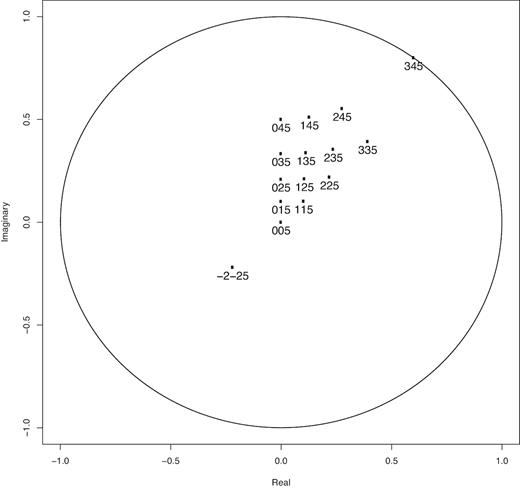
Overview of investigated ellipticity values.
An overview of the tested parameter combinations.
| Combination | u | v | s |
|---|---|---|---|
| 1 | 0 | 0 | 5 |
| 2 | 0 | 1 | 5 |
| 3 | 0 | 2 | 5 |
| 4 | 0 | 3 | 5 |
| 5 | 0 | 4 | 5 |
| 6 | 1 | 1 | 5 |
| 7 | 1 | 2 | 5 |
| 8 | 1 | 3 | 5 |
| 9 | 1 | 4 | 5 |
| 10 | 2 | 2 | 5 |
| 11 | 2 | 3 | 5 |
| 12 | 2 | 4 | 5 |
| 13 | 3 | 3 | 5 |
| 14 | 3 | 4 | 5 |
| 15 | -1 | -2 | 5 |
We pair this with the sigma values σ = 0.05, 0.1, 0.25, 0.5, 0.75, 1, 1.5, 2, 3, 5, using the sigma value for the sampling from the mean values u, |$v$|, and s. To minimize variance of the experiment, we choose a sufficiently large sample size for each combination of n = 25 000. Each estimator is tested against the true ellipticity value and an absolute error measure is taken. The mean value of these errors can be found in the Tables 8–11.
Error table for the different estimators and sigma values for u = −2, |$v$| = −2, and s = 5, for example ε = −0.219 224 − 0.219 224i.
 |
|
Error table for the different estimators and sigma values for u = −2, |$v$| = −2, and s = 5, for example ε = −0.219 224 − 0.219 224i.
|
|
We discuss a selected pairings of values only, which serve as examples for the various ellipticity locations. The full set of tables can be provided upon inquiry.
To investigate the influence of negative values on the estimators, we have included an example with negative mean values u = −1, |$v$| = −2, and s = 5. The results are listed in Table 8. In comparison to the positive values, we see that the negative values make very little difference in the performance of the estimators. As u and |$v$| are rather directly estimated through the values x and y, the negative sample values directly translate into the estimation. We will therefore consider positive mean values without loss of generality.
The colour coding is designed to help scan the experiment results more easily. Higher error averages are in red, and gradually turning into green background colouring the lower the absolute error gets. The main estimator we compare our newly designed estimators against, is the unaltered |$\widehat{\epsilon }_{I}$| or the scaled version, since they are considered to be the strongest contenders for a new estimator against the cruder direct version based on |$\widehat{\epsilon }_{II}$|, which simply plugs in the single sample values into the ellipticity formula.
Around the origin u = 0, |$v$| = 0, and s = 5 in Table 9, we can see mostly indifference between the estimators, with a bit of preference for estimators 30–32 and 37–38. Also the differences in performance naturally increase for larger variances. In this range, there is a slight preference for 11, 15, 17, and 19 as well as 23–29 in addition to the overall 30–32 performances. This however may be due to the scaling function in certain estimators, which for an ellipticity in the origin will automatically create better results. Therefore, this set of results has to be taken with a grain of salt.
Error table for the different estimators and sigma values for u = 0, |$v$| = 0, and s = 5, for example ε = 0 + 0i.
 |
|
Error table for the different estimators and sigma values for u = 0, |$v$| = 0, and s = 5, for example ε = 0 + 0i.
|
|
When we move a little further away from the origin, the picture changes a little in Table 10. While estimators 23–29 are still performing as well or better as the original estimators and their modifications, especially for larger sigmas (for small sigmas there is little difference to the unbiased estimator, as the derivatives are based upon |$\widehat{\epsilon }_{I}$|), we see the addition of estimators 11, 15, 17, 19, and 23–29. Furthermore, estimator 44 works fairly well, with decreasing performance for larger variances. Also the average estimators from number 48 onwards perform consistently well.
Error table for the different estimators and sigma values for u = 0, |$v$| = 3, and s = 5, for example ε = 0 + 0.333i.
 |
|
Error table for the different estimators and sigma values for u = 0, |$v$| = 3, and s = 5, for example ε = 0 + 0.333i.
|
|
For the combination u = 2, |$v$| = 2, and s = 5 the same candidates stand out again in Table 11, delivering sensible alternatives to the original estimators. We do recognize some issues with estimators 19 and 21, who grossly misestimate the true ellipticity value for larger sigma values. For number 19 this might be due to singularities, but it seems there is some intrinsic problem with the estimator 21, which produces arbitrarily large values.
Error table for the different estimators and sigma values for u = 2, |$v$| = 2, and s = 5, for example ε = 0.219 + 0.219i.
 |
|
Error table for the different estimators and sigma values for u = 2, |$v$| = 2, and s = 5, for example ε = 0.219 + 0.219i.
|
|
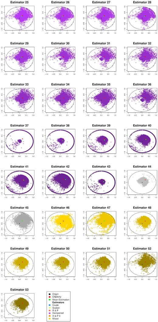
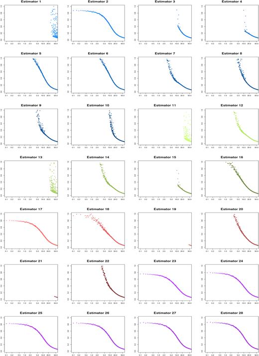
In the matrix of scatter plots in Figs 2 and 3 (continued), we can see the behaviour of each estimator with a distribution of empirical ellipticities. Each individual estimate for a random experiment is marked by a blue dot, the true value is marked by a single red spot. Furthermore, we have added the average of all estimates of all random experiments, to give a sense of what the bias is.
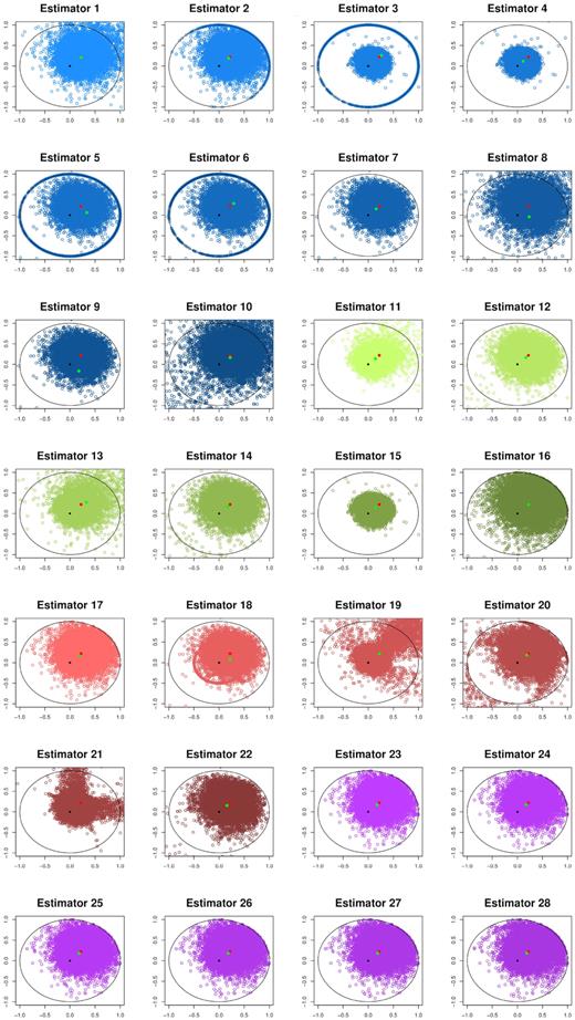
Matrix of estimators’ 1–28 performance, with true values and bias added. Real x-axis versus imaginary y-axis.
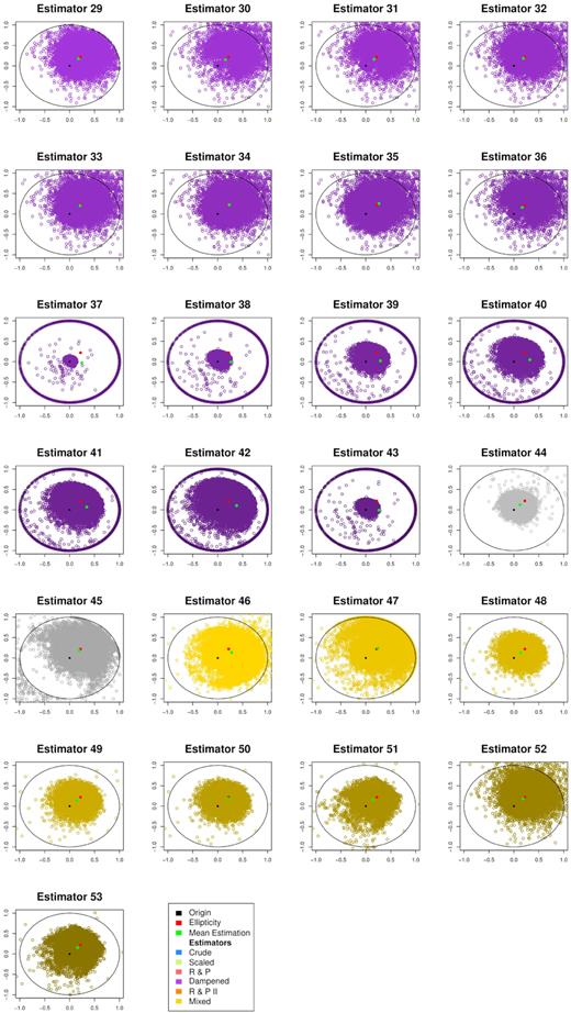
Matrix of estimator’ 29–53 performance, with true values and bias added. Real x-axis versus imaginary y-axis.
It becomes evident where some estimators have their largest shortcomings by observing their distribution. The unscaled estimators often overshoot the feasible range of the unit circle, and therefore produce avoidable overestimation. On the other hand some of the scaling approaches, especially the parameter scaling approaches distort the actual value. We can see this through the way the scaled values on the unit circle boundary exhibit a grossly miscalculated angle.
On the other hand, we can see some decent performances, where the individual estimates exhibit a tighter grouping around the true value without producing a noticeable bias shift. These candidates seem promising, and we will review their practical potential by looking into their range-specific behaviour. We see this confirmed at the border of the unit circle with parameter values u = 3, |$v$| = 4, and s = 5 in Table 12. The problems with estimators 19 and 20 persist for this configuration, yet our favoured estimators exhibit a decent performance when compared to the original estimators. Additionally, the |$\widehat{\epsilon }_{II}$| based estimators perform rather well for the mid-range variance values around σ = 1.
Error table for the different estimators and sigma values for u = 3, |$v$| = 4, and s = 5, for example ε = 0.6 + 0.8i.
 |
|
Error table for the different estimators and sigma values for u = 3, |$v$| = 4, and s = 5, for example ε = 0.6 + 0.8i.
|
|
3.1 Non-perfect ellipticity
Sampling from the means u, |$v$|, and s via a normal distribution implicitly assumes the shape of the galaxies to be perfectly elliptical, which of course is a strong assumption. We have therefore tested a simulation in which the X, Y, and Z samples are distributed according to a non-central Student-t distribution (Gosset 1908).
We may assume the previous values u, |$v$|, and s as the means, as well as the standard deviation σ and retrieve the corresponding characterizing parameters ν and μ which are the degrees of freedom and non-centrality parameters, respectively.
Assume that X ∼ S(νX, μX), Y ∼ S(νY, μY), and Z ∼ S(νZ, μZ). By setting Var[X] = Var[Y] = σ2, Var[Z] = 4σ2, |$\mathbb {E}[X] = u$|, |$\mathbb {E}[Y] = v$|, and |$\mathbb {E}[Z] = s$|, we can estimate values of ν and μ. We would like to note that we have to assume σ > 1 due to the nature of the non-central Student-t distribution. This enables us to do the exact same experiment we have done with the assumption of normally distributed measurements.
We have listed the results as before for an example problem with values u = 2, |$v$| = 2, and s = 5 across different standard deviations, which translate to the SNR values 4.7619,4,3.333,2.5,2,1.75,1.5,1.25, and 1. The matrix can be seen in Table 13.
Error table for the different estimators and sigma values for u = 2, |$v$| = 2, and s = 5, for example ε = 0.219 + 0.219i, assuming Student-t distribution.
 |
|
Error table for the different estimators and sigma values for u = 2, |$v$| = 2, and s = 5, for example ε = 0.219 + 0.219i, assuming Student-t distribution.
|
|
Furthermore, we have repeated the graphic representation of the estimator spread and behaviour in Figs 4 and 5. The colour scheme remains the same as previously introduced to help distinguish the classes of estimators.
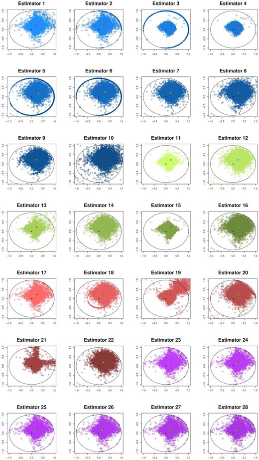
Matrix of estimators’ 1–28 performance, with true values and bias added for the Student-t distribution. Real x-axis versus imaginary y-axis.
Matrix of estimators’ 29–53 performance, with true values and bias added for the Student-t distribution. Real x-axis versus imaginary y-axis.
The most striking change we can observe in the tables is how much more vulnerable the estimators have become to low-SNR values. This is especially visible in the |$\widehat{\epsilon }_{I}$| based estimators. The scaling approaches with dampening parameter seem to work better across all SNR ranges, even though sometimes only slightly so. This of course depends on the position of the true mean values. The closer the true ellipticity gets to the unit circle boundary, the better the scaling approach works in comparison to the original estimator. We have observed similar behaviour in the normal sampling experiment, but here we restricted ourselves to only certain value pairings, full error tables may be provided upon request.
In the figures, we see much of the behaviour from previous experiment, yet notice a recurring pattern of the individual estimators, which seem to group along the axes, giving the estimate cloud a diamond-shaped appearance. However, generally most of the scaling approaches seem to be doing their job and resize estimates based on measurements exceeding the unit circle to a sensible new approximation.
3.2 Performance by signal-to-noise ratio
With the investigation of the performance of the estimators for predetermined parameter sets complete, we have settled on a number of promising new candidates. While the original estimator delivers a solid performance, it neglects the potential infeasibility of output values, or the input’s violation of the ellipticity formula rules.
This procedure of procuring the necessary randomized observations ensures that we do not focus on singular areas and parameter combinations as before. This should provide a more complete view of how the estimators are likely to perform in practical applications.
We have settled on the standard deviations σe = 0.2 and σo = 1 and an SNR range of [0, 100] which should cover most values of interest. Since there are more points to investigate, we have lowered the sample size for each individual SNR to n = 500 for a first glance at the estimator performance in relation to the SNR. The results are visualised in Figs 6 and 7, where we split the estimators into two groups for better visibility.
The SNR versus mean absolute errors for estimators 1–28, normal distribution. SNR range on x-axis versus average absolute error on y-axis.
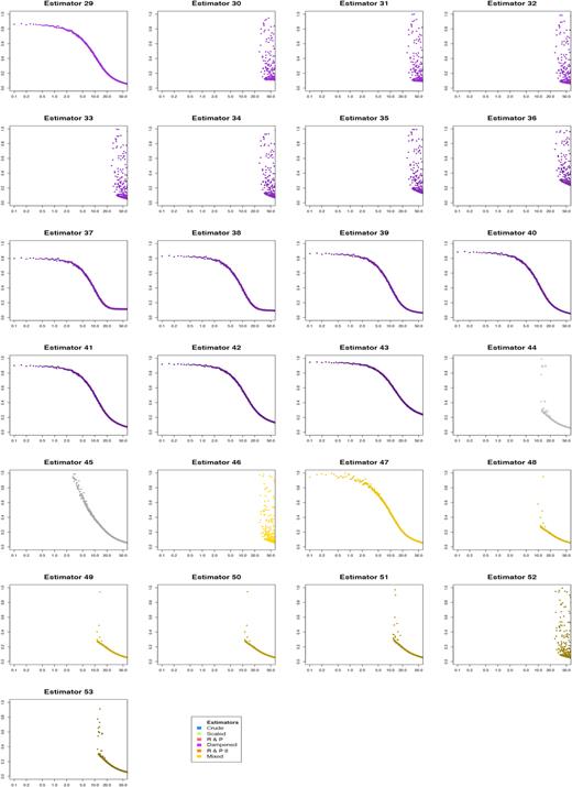
The SNR versus mean absolute errors for estimators 29–53, normal distribution. SNR range on x-axis versus average absolute error on y-axis.
The sample size mainly controls the variance of the error dots in the plots. We split the plot matrices in two groups, 1–28 and 29–53. We observe the generally expected shape of the curve for most estimators, with higher values of s = SNR*σo the absolute error subsides. Since a higher s value diminishes the ellipticity ε, as it is only recurring in the denominator of the fraction, we get a smaller spread in initial samples.
Furthermore, we can see that some estimators are susceptible to failure, mostly due to the lack of a scaling mechanism. This becomes visible in some of the outliers, which seem to become more frequent as s → 0, leading to a divergence of the ellipticity value. We therefore measure the success of the other estimators mainly against |$\widehat{\epsilon }_{2}$| and |$\widehat{\epsilon }_{5}$|, since the original unbiased estimator fails for ellipticities around the unit circle (as previously discussed).
We see many of the trends from the static parameter tables confirmed. The odd numbered estimators based on the unbiased estimators 15, 17, 19, 21, and 23 for example exhibit a lower mean absolute error, which is especially visible in the lower SNR regions near the coordinate origin. The y-intercept for |$\widehat{\epsilon }_{2}$| is between 0.9 and 1, a value which a number of estimators seem to underbid.
For the parameter and result based scaling techniques, we see good success in estimators such as number 44 or 49, especially for the tail regions there seems to be a fairly quick convergence. Unfortunately, the approach does not seem stable for small SNR values, as the error values scatter a lot more and eventually break due to missing values in the experiment output. We now move on to a direct comparison of all the methods, to give us an impression of how the performance relate to one another, and if there is significant potential for the newly constructed empirical ellipticities.
Figs 8 and 9 depict all approaches in a single frame, showing the averages of absolute error and variance, respectively. The crude and unbiased estimators (|$\widehat{\epsilon }_{2}$| to be precise) are highlighted in red and superimposed over the bulk of the other estimators. The plots primarily give us a first glance at the outcome of the experiment, before we highlight single estimation approaches. As we can see, several monochrome point clouds shape up underneath the red line plots. This is a first indication that stronger estimators for arbitrary values exist.
![Average absolute error, SNR = [0, 100], logarithmic x-scale. SNR range on x-axis versus average absolute error on y-axis.](https://oup.silverchair-cdn.com/oup/backfile/Content_public/Journal/mnras/484/3/10.1093_mnras_stz218/1/m_stz218fig8.jpeg?Expires=1750477589&Signature=plOAYQmJWHTxaPwmCs9yxJXd8iJhuM87AghITahdE9MEgc-43bHZcmeBm3iH7jsS-9~SEj4w15Evgg8H1zZCF~dpAtBayeMd4peisR4BqZVdqhqpNvfTPWHqqzxU-jv5y8h-mAcNTOldl4Cqess19JWpN7U2lA8-HfBLpLEsTgpZmnPvp10xaW9rpwrAaGBo2mjAyTjQSykaqZgb19prcjmfe7PlEallOm~sRsBwSqmO0mEtuux7XWbCf1MA2cO3J6fADIqgzvFGRzJtRfQyfF5zniF2WyR~9-LX239J2qF7SSgXTm4UeOMW~fo5lkd6orwyOiQYcgpLbe5cis7JiQ__&Key-Pair-Id=APKAIE5G5CRDK6RD3PGA)
Average absolute error, SNR = [0, 100], logarithmic x-scale. SNR range on x-axis versus average absolute error on y-axis.
![Average estimator variance, SNR = [0, 100], logarithmic x-scale. SNR range on x-axis versus average variance on y-axis.](https://oup.silverchair-cdn.com/oup/backfile/Content_public/Journal/mnras/484/3/10.1093_mnras_stz218/1/m_stz218fig9.jpeg?Expires=1750477589&Signature=3XTlDw8lF3V939nFxDq6RznXDsdXj7nJAl42dMJbFQGXvQ5gFBL-eUcQRRAH987oat3nBL0Zk3~zTZAokXyvp6C3cQdKpKs2B6s9kv8YL-Ctl60yBQEcYUDm7C1JJ7Lq3jlH1gdIDq36hK~Zx~zn9LlXkvZlI1E0gp0XcVTXoWtLBRviPwQzIebSTBDM6oWwlcaUtvDb4kRPDXYs6QralJku3Jtp66mc5F5FpLfqU0R5XWI5SxPKjZv4xnByFNU5jl0FftFS4hW3~KIbK6v-Sc0-PHjA1f7PKebcK2gJZnpnVQQYh64K3YlIS7qfecuhYNGF4HIvl2Axii2LaUxvjA__&Key-Pair-Id=APKAIE5G5CRDK6RD3PGA)
Average estimator variance, SNR = [0, 100], logarithmic x-scale. SNR range on x-axis versus average variance on y-axis.
We single out the approaches found to deliver the strongest results, based on the error tables for fixed ellipticity values and the individual and comparative plots. We narrow down the observed estimators to the preferred selection, in order to make the plots more readable. Since the SNR area of interest is below 30, we have omitted the larger tail of the plot, which served to check the estimators for convergence. In the focus plots, we get a much clearer picture of the comparative performance of the estimators, depicted in Figs 10 and 11.
![Average absolute error of selected estimators, SNR = [0, 30]. SNR range on x-axis versus average absolute error on y-axis.](https://oup.silverchair-cdn.com/oup/backfile/Content_public/Journal/mnras/484/3/10.1093_mnras_stz218/1/m_stz218fig10.jpeg?Expires=1750477589&Signature=K2oQPJd8QFSvNVQ0AobnE~Kpbtwucqojf2vU3LTGosOTnUdhonkmFJYfdrGCCjWQhn7L2JGPO5Ym~o1jbY1aBvy5w4KQaoiiaWBaA1UI49S4CBxM6uAm0HF2KJ9agN6T7EnEmaZu3XXptestZs9cjdoTeVK9~~-MMY-QxBj~VJjfOI9MATiqthBq1s3gh5HXJUYm6O9lEo18R-rNFUTCziE0~~xpwYOcD6xf~h0aMkr~AqbESOX4RU2YB~CGqnG5Dxkt3imyMtfkIfKZVoLtXfIsrCVnWKioPt4oit2DaXQt~QAjs3A-HFObFL9yRaLvrCsAuo1a0cKnaGmW2THeTQ__&Key-Pair-Id=APKAIE5G5CRDK6RD3PGA)
Average absolute error of selected estimators, SNR = [0, 30]. SNR range on x-axis versus average absolute error on y-axis.
![Average variance of selected estimators, SNR = [0, 30]. SNR range on x-axis versus average variance on y-axis.](https://oup.silverchair-cdn.com/oup/backfile/Content_public/Journal/mnras/484/3/10.1093_mnras_stz218/1/m_stz218fig11.jpeg?Expires=1750477589&Signature=t8rU19vqCi8o-G~uTpcDq17WyCyb2O7rKAs-SYDs9iwZLMtnFqlwbynfH~qMmUlhe8l7glLeXUI1hs51RtamNC6YQEjfwWMU3nSbOiXalj23XgVBKT-Bk2Q04bEWQ7fpWZ8fnoJ~aY6A0rmU96hyJBe8-TaOGr-y9P5y2e2fQYWcS7bALkt19YKqk5xV1xs~e0Hso636aUeQg7gJd9xNx7WLUdF7JhW9iqGvFDjdcq5h79MTgr1eC-k369QCJPTAvbHJiVOiJbtGq~k5XLJR5gE5gLQKR1OBetBUGzbYu1iD~OQFNjD062L0qEheGHxxIYt-6Dp7i9edKhcQuh048w__&Key-Pair-Id=APKAIE5G5CRDK6RD3PGA)
Average variance of selected estimators, SNR = [0, 30]. SNR range on x-axis versus average variance on y-axis.
Starting with the largest SNR, we can see that estimator 39 exhibits the lowest average error, converging towards zero the fastest. This effect takes effect roughly from SNR = 20 onwards, whereas the estimator has a seemingly weaker performance for smaller SNR values, for example, higher standard deviations, eventually matching the benchmark of |$\widehat{\epsilon }_{II}$|. The variances in this interval are very tightly grouped, with estimator 37 narrowly beating out the aforementioned approach number 39.
The next interval which is clearly marked by a difference in accuracy covers SNR = [10, 20], edging closer to the area of practical applicability. Both the scaled estimator number 15 and averaged estimator 50 show a reduction in absolute error by as much as |$25-30{{\ \rm per\ cent}}$|. The variance plots show an even clearer gap to the next best competitor, where the faint beige coloured error points of estimator 50 seem to surpass the scaled unbiased estimator once again, by roughly |$60{{\ \rm per\ cent}}$|. It should be stated at this point that there are some outliers visible in the plot from both approaches, suggesting robustness issues. This becomes even more evident when both estimators fail due to missing values being introduced, thus questioning the practical use of those estimators for SNR ≤10, and the robustness in general.
Lastly, and most importantly we focus on [0, 10], representing the interval of the highest practical interest. Once more it becomes clear which approach delivers the best results, as estimator 23 undercuts the other approximations consistently throughout the range in question. The absolute difference is about 0.075–0.1, which is roughly an error reduction of |$10{{\ \rm per\ cent}}$|. Perhaps more importantly, we cannot see the same amount of outliers as for estimators 15 and 50, suggesting greater stability of the estimators, less susceptible to variances in the input parameters. Additionally, we see a reduction in variance, as the estimator 23 exhibits the lowest variances for the range [0, 10]. The similar estimators 24, 25 and onwards perform similarly, albeit less accurately. Possibly the parameter β = 0.25 is not yet optimally chosen, and can be altered for even better results in the future.
We have analysed and discussed the test results for all newly suggested approaches, and have settled on a recommended estimation technique for a given SNR range. As a last step we have averaged the mean absolute values across different SNR intervals, thus putting our observations from the visualised results in comprehensible numbers. Table 14 lists the mean error results, whereas Table 15 contains the variances summarized in the same way.
Average absolute error over the respective SNR ranges.
| SNR range | ||||||
|---|---|---|---|---|---|---|
| [0, 100] | [0, 50] | [0, 30] | [0, 15] | |||
| Estimator number | Crude | 2 | 0.061 64 | 0.100 51 | 0.147 69 | 0.237 46 |
| 5 | 0.205 97 | 0.389 31 | 0.629 09 | 1.197 73 | ||
| Scaled | 15 | 2.04E + 82 | 4.08E + 82 | 6.80E + 82 | 1.37E + 83 | |
| R & P | 17 | 0.052 87 | 0.083 20 | 0.119 72 | 0.189 52 | |
| 19 | 4.95E + 304 | 8.23E + 155 | 1.96E + 104 | 1.37E + 83 | ||
| Dampening | 23 | 0.049 35 | 0.076 24 | 0.108 38 | 0.169 60 | |
| 24 | 0.051 94 | 0.081 37 | 0.116 76 | 0.184 46 | ||
| 25 | 0.054 96 | 0.087 33 | 0.126 43 | 0.201 27 | ||
| 37 | 0.038 98 | 0.076 75 | 0.124 79 | 0.221 75 | ||
| 39 | 0.049 00 | 0.089 06 | 0.139 26 | 0.238 55 | ||
| 41 | 0.07119 | 0.113 96 | 0.165 99 | 0.264 20 | ||
| R&P II | 44 | 3.29E + 82 | 6.59E + 82 | 1.10E + 83 | 2.21E + 83 | |
| Mixed | 48 | 1.75E + 82 | 3.51E + 82 | 5.86E + 82 | 1.18E + 83 | |
| 50 | 1.66E + 82 | 3.33E + 82 | 5.56E + 82 | 1.12E + 83 | ||
Average variance over the respective SNR ranges.
| SNR range | ||||||
|---|---|---|---|---|---|---|
| [0, 100] | [0, 50] | [0, 30] | [0, 15] | |||
| Estimator number | Crude | 2 | 0.157 50 | 0.264 57 | 0.376 84 | 0.562 44 |
| 5 | 0.181 41 | 0.312 17 | 0.455 10 | 0.708 01 | ||
| Scaled | 15 | 1.37E + 38 | 2.74E + 38 | 4.57E + 38 | 9.17E + 38 | |
| R & P | 17 | 0.146 49 | 0.242 70 | 0.341 25 | 0.500 89 | |
| 19 | 6.77E + 163 | 1.62E + 75 | 2.36E + 49 | 9.17E + 38 | ||
| Dampening | 23 | 0.141 05 | 0.231 73 | 0.322 96 | 0.467 67 | |
| 24 | 0.145 15 | 0.240 03 | 0.336 92 | 0.493 63 | ||
| 25 | 0.149 61 | 0.249 00 | 0.351 70 | 0.519 67 | ||
| 37 | 0.197 66 | 0.261 13 | 0.344 31 | 0.520 14 | ||
| 39 | 0.159 69 | 0.250 69 | 0.359 27 | 0.559 42 | ||
| 41 | 0.179 86 | 0.295 98 | 0.418 50 | 0.619 58 | ||
| R & P II | 44 | 2.21E + 38 | 4.43E + 38 | 7.38E + 38 | 1.48E + 39 | |
| Mixed | 48 | 2.35E + 38 | 4.71E + 38 | 7.87E + 38 | 1.58E + 39 | |
| 50 | 2.24E + 38 | 4.48E + 38 | 7.47E + 38 | 1.50E + 39 | ||
Most strikingly, we recognize the issues of stability, which are visible for estimators 15, 17, 44, 48, and 50. The tremendously high errors and variances are due to the inherent flaw to these estimation techniques, that they allow for arbitrarily large estimates, which can be caused by unchecked or unscaled problematic input parameters. Starting with the largest range of SNR in [0, 100], we recognize the lowest average error values from estimators 37, 39, closely followed by number 23, all offering a better option than the benchmark |$\widehat{\epsilon }_{2}$|. However, this behaviour does not persist for all SNR intervals. We had realized earlier that the estimators 37 and 39 give their strongest performance only from SNR = 30 onwards, which lies outside of the realistically sensible ranges. If we draw the circle a little bit closer, and omit results larger than SNR = 50 estimator 23 delivers the best results, undercutting all other approaches. As we reduce the investigated interval, the effect becomes stronger, with estimator 23 reducing the error of |$\widehat{\epsilon }_{2}$| by almost |$29{{\ \rm per\ cent}}$| for the narrowest range [0, 15].
For the variance the observations are even clearer, here the scaled estimator 23 exhibits the smallest variance for all listed ranges. Realistically speaking, the smallest range [0, 15] is of the highest significance for practical applications, therefore leaving us with a clear recommendation on which estimator has the largest potential in practice.
In a more categorical overview, we try to investigate how the different types of estimators perform in a given setting. The first category we dubbed ‘crude’ estimators, due to their straightforward nature and simplistic scaling and censoring approach, do not perform remarkably better than any baseline method. In the ‘parameter-only’ scaling section estimator 15 alone performed noteworthily better than the baseline approach. The more sophisticated estimators which scale either parameters, or the entire result based on certain parameter values perform considerably better. This may lead us to the conclusion that result scaling is the general approach, a claim that is verified by the section of exclusively result-scaling approaches. Censoring on the other hand does only seems to slightly increase performance, certainly not to a degree that would allow for routine discarding of data. Another problem with data censoring is the censoring criterion. While X2 + Y2 < Z2 effectively works for the Type 2 basic estimator, it does not necessarily omit corrupted data for the Type 1 estimator. The most complex estimators of the second to last category perform best in the very high SNR region, beginning with a ratio of 17 or higher. This puts them outside the most common region of ratio values.
What strikes us is that the result-only scaling introduces only very little bias. As the basic estimator is unbiased, it has to be expected to trade some degree of underestimation of the ellipticity (as we always scale down) for a generally more accurate result overall, observable in Fig. 2. However, the slight bias only occurs in the individual ellipticity estimation of a galaxy, and as the scaling is centred towards the origin (for example only the radius, not the angle is corrected), no bias will appear in an average of galactic ellipticities. The dampening parameters introduced as β could for this purpose be analysed more thoroughly, as the values we have chosen were somewhat arbitrary to give us a more diverse picture. It is imaginable that a dependence on the SNR or standard deviation σ could be derived for an optimal β either empirically or theoretically.
Other scaling functions besides the inverse tangent function may be considered as well, as only the asymptotic values of the scaling function are fixed. A number of different functions with the correct properties and numerous optimisation parameters may be tested, to increase accuracy, while even further minimizing variance and bias of the estimation. We may consider this question in further work, as this would have gone beyond the scope of this paper.
At this point, we want to stress that these simulation are highly idealized. The assumption of normal distributed samples corresponds to galaxies exhibiting the shape of perfect ellipses, which in nature obviously will not have to be the case. Furthermore, the process of deriving the measurement values from the actual galaxy is much more complex than our simulation does justice. Various steps along the actual process of obtaining measurement may introduce bias or distortions which this experimental set-up can not reproduce. The performance analysis of this section should be seen as a very simple assessment of theoretical applicability of these approaches, rather than emulating practical effects.
4 CONCLUSIONS
In this paper, we have introduced and discussed a number of extensions to the base estimators |$\widehat{\epsilon }_{I}$| and |$\widehat{\epsilon }_{II}$|. Due to the limited sample size, strictly speaking we were not able to employ common statistical methods. We employed scaling and censoring techniques based on the conditions the parameters have to fulfill, or are at least desirable to the coherence of the input data.
As we have demonstrated in the simulation experiments, and have explained in the discussion part of Section 3, some of the proposed techniques have definite potential for practical use. Both for fixed underlying means and randomised ellipticities, we see strong performances for a number of our proposed approaches, which retain sufficient numerical stability to be of use in application scenarios.
Other application areas may be considered as well, as the estimation problem is not strictly bound to the original problem anymore. We would have to reconfigure the scaling criterion according to the new application, and might reconsider the scaling function, but the general approach may be much more widely applicable.
We believe there might be even further room for improvement, if the estimators get used in accordance to the SNR or true ellipticity region (for example r ≈ 0 or r ≈ 1). As the variance is known in most cases, it is possible to create confidence areas of the true location of the ellipticity. Hence, an estimation selection algorithm could be developed, which based on the known input factors chooses the optimal approach. As touched upon in the simulation section, scaling functions other than the inverse tangent function may be considered as well. As the dampening parameter β in the most successful category of estimators had tremendous influence over the performance of the estimator, an optimal parameter dependent on σ would be desirable and could help to minimize. We have given first possible starting points with respect to selective estimators.
ACKNOWLEDGEMENTS
We would like to thank Sarah Bridle and Nicolas Tessore for bringing this problem to our attention. We also thank them for their helpful comments which greatly contributed to this paper. We would furthermore like to express our thanks to the referee, whose comments were very constructive and helped to improve this paper.
