


Abstract
The duration of quasar accretion episodes is a key quantity for distinguishing between models for the formation and growth of supermassive black holes, the evolution of quasars, and their potential feedback effects on their host galaxies. However, this critical time-scale, often referred to as the quasar lifetime, is still uncertain by orders of magnitude (|$t_{\rm Q} \simeq 0.01\, {\rm Myr} - 1\, {\rm Gyr}$|). Absorption spectra of quasars exhibiting transmission in the He ii Ly α forest provide a unique opportunity to make precise measurements of the quasar lifetime. Indeed, the size of a quasar’s He ii proximity zone, the region near the quasar where its own radiation dramatically alters the ionization state of the surrounding intergalactic medium (IGM), depends sensitively on its lifetime for |$t_{\rm Q}\lesssim 30\, {\rm Myr}$|, comparable to the expected e-folding time-scale for SMBH growth |$t_{\rm S} =45\, {\rm Myr}$|. In this study, we compare the sizes of He ii proximity zones in the Hubble Space Telescope (HST) spectra of six |$z$| ∼ 4 quasars to theoretical models generated by post-processing cosmological hydrodynamical simulations with a 1D radiative transfer algorithm. We introduce a Bayesian statistical method to infer the lifetimes of individual quasars which allows us to fully marginalize over the unknown ionization state of the surrounding IGM. We measure lifetimes |$0.63^{+0.82}_{-0.40}$| Myr and |$5.75^{+4.72}_{-2.74}$| Myr for two objects. For the other four quasars, large redshift uncertainties undermine our sensitivity allowing us to only place upper or lower limits. However, a joint analysis of these four systems yields a measurement of their average lifetime of |$\langle t_{\rm Q}\rangle = 1.17^{+1.77}_{-0.84}$| Myr. We discuss our short |${\sim } 1\, {\rm Myr}$| inferred lifetimes in the context of other quasar lifetime constraints and the growth of SMBHs.
1 INTRODUCTION
Quasars are the most luminous non-transient sources of radiation in the Universe. It is believed that they not only played an important role in the evolution of cosmic structure on all scales, for instance dramatically changing the ionization and thermal state of the surrounding intergalactic medium (McQuinn et al. 2009; Compostella, Cantalupo & Porciani 2013; Khrykin et al. 2016; Chardin, Puchwein & Haehnelt 2017; Davies, Furlanetto & Dixon 2017; D’Aloisio et al. 2017; Khrykin, Hennawi & McQuinn 2017; La Plante et al. 2017), but also possibly regulating star formation in galaxies (Springel, Di Matteo & Hernquist 2005; Hopkins et al. 2006). However, many questions about the nature of quasars and their evolution remain unanswered. For example, the existence of SMBHs with masses MBH ≃ 109 − 1010M|$\odot$| (Fan et al. 2001, 2004; Mortlock et al. 2011; Venemans et al. 2013; De Rosa et al. 2014; Wu et al. 2015; Bañados et al. 2018) already at |$z$| ∼ 6–7 poses a challenge for current theories of SMBH formation, requiring very massive initial black hole seeds and accretion of matter on time-scales comparable to the Hubble time (Hopkins & Hernquist 2009; Volonteri 2010, 2012). Solving this puzzle is impossible without constraints on the characteristic time-scale over which accretion on to SMBHs occurs.
A holy grail would thus be a direct measurement of the lifetime tQ of quasars at high-redshift, or more precisely the duration of their individual accretion episodes. This would shed light on triggering and feedback mechanisms (Springel et al. 2005; Hopkins et al. 2006), on how gas funnels to the centres of galaxies, and on the structure of the inner accretion disc (Goodman 2003; Hopkins & Quataert 2010). Unfortunately, the best currently available estimates on the time-scales governing quasar activity are uncertain by several orders of magnitude (see Martini 2004 for a review). For instance, studies of quasar demographics which attempt to model the quasar luminosity function and/or quasar clustering (Haiman & Hui 2001; Martini & Weinberg 2001) constrain the total integrated time that a galaxy hosts an active quasar, known as the quasar duty cycle tdc. These studies often come to very different conclusions depending on the particular assumptions made in the modelling, but constraints are in the range |$t_{\rm dc} \approx 1\, {\rm Myr}-1\, {\rm Gyr}$| (Yu & Lu 2004; Adelberger & Steidel 2005; Croom et al. 2005; Shen et al. 2009; White et al. 2012; Conroy & White 2013; Cen 2015; La Plante & Trac 2016). In particular, the very strong clustering of quasars measured at |$z$| ∼ 4 implies tdc ∼ 1 Gyr (Shen et al. 2007; White, Martini & Cohn 2008), much higher than estimates of this duty cycle at lower-|$z$|, and seems to require an extremely tight relationship between the black hole mass MBH and the halo mass Mhalo (White et al. 2008). It is important to note that while these demographic studies constrain the quasar duty cycle tdc, they are insensitive to the duration of individual accretion episodes tQ, which theoretical models suggest could be much shorter (Ciotti & Ostriker 2001; Novak, Ostriker & Ciotti 2011).
Previous studies employing a variety of techniques have found tentative evidence for short episodic quasar lifetimes tQ. For example, recent work by Schawinski et al. (2010, 2015) based on light traveltime arguments in active galactic nuclei (AGN) host galaxies argues for quasar variability on time-scales of tQ ≃ 0.1 Myr. However, plausible alternative scenarios related to AGN obscuration could explain those observations without invoking short time-scale quasar variability, and furthermore the giant |${\sim } 500\, {\rm kpc}$| Ly α nebulae discovered around |$z$| ∼ 2 quasars (Cantalupo et al. 2014; Hennawi et al. 2015) imply quasar lifetimes of ≳1 Myr, at odds with these short inferred lifetimes. Oppenheimer et al. (2018) (see also Gonçalves, Steidel & Pettini 2008) argued that the high incidence of strong high-ionization absorption lines in the circumgalactic medium of galaxies provides evidence for relic light echoes from an AGN, implying tQ ≲ 1 Myr, but the nature of these absorbers is a subject of intense debate and many models manage to explain them (Stern et al. 2016, 2018; Mathews & Prochaska 2017; McQuinn & Werk 2018) without invoking a previously active AGN. Finally, the presence of high equivalent width Ly α emitters (LAEs) near hyper-luminous quasars has been attributed to quasar-powered fluorescence and invoked to argue for quasar lifetimes of 1 ≲ tQ ≲ 30 Myr (Trainor & Steidel 2013; Borisova et al. 2016). However, the expected boost due to the quasar illumination is inconsistent with the much brighter observed Ly α luminosities of these LAEs, strongly suggesting that these sources are powered intrinsically and not by the nearby quasar (but see Adelberger et al. 2006). To summarize, all of the aforementioned methods are indirect and often involve model-dependent assumptions, such that plausible alternative scenarios can be invoked to explain the observations.
On the other hand, the ionization state of the IGM in quasar environs provides a powerful method to estimate quasar lifetimes. For example, using the observational survey data presented in Schmidt et al. (2017), Schmidt et al. (2018) carefully analysed the He ii Ly α transverse proximity effect (TPE; Jakobsen et al. 2003; Worseck & Wisotzki 2006; Schmidt et al. 2017), which is the increased IGM He ii Ly α transmission in a background quasar sightline due to the enhancement of the radiation field from a foreground quasar. They found that the strength of the TPE signal exhibits a degeneracy between quasar lifetime and the solid angle of the UV emission (or, equivalently, the fraction of quasars that are obscured), and uncovered a possible bimodality in quasar emission properties whereby some quasars appear to be unobscured and relatively long lived (tQ ≳ 10 Myr), whereas others are either younger (tQ ≲ 10 Myr) or highly obscured.
This degeneracy with quasar obscuration can be removed if one instead considers the line-of-sight (LOS) proximity effect, since the background quasar illuminates the IGM along our sightline towards Earth by construction. Indeed, the LOS proximity effect in the H i Ly α forest at |$z$| ≃ 2–4 (Carswell et al. 1982; Bajtlik, Duncan & Ostriker 1988) has been used to constrain tQ, but it provides only weak lower limits on tQ ≳ 0.01 Myr (Dall’Aglio, Wisotzki & Worseck 2008). This limit results from the fact that in order to produce a detectable LOS proximity effect the quasar must shine longer than the time it takes the IGM to attain ionization equilibrium with the enhanced quasar radiation, the so-called equilibration time-scale |$t_{\rm eq} \simeq \Gamma _{\rm HI}^{-1}$|. Given the measurements of the UV H i background photoionization rate |$\Gamma _{\rm HI}^{\rm bkg} \simeq 10^{-12}{\rm s^{-1}}$| (Becker et al. 2013) at |$z$| ≃ 3–5, the H i proximity effect is, in principle, detectable, provided that tQ ≳ 0.01 Myr. This argument provides the basis for the recent discovery of a population of very young quasars (tQ ≲ 0.01–0.1 Myr) at |$z$| ≃ 6 (Eilers et al. 2017; Eilers, Hennawi & Davies 2018) as inferred from small sizes of their LOS proximity zones. It remains unclear whether a similar population of young quasars exists at lower redshift. It could be that they have only been uncovered at |$z$| ∼ 6 because the much higher Ly α optical depth of the surrounding IGM makes their small proximity zones particularly conspicuous. In addition, a more precise constraint on lifetime can be obtained if one combines the analysis of high-|$z$| H i proximity zones with the study of damping wing signatures in the quasar spectra (Davies et al. 2018). This approach, applied to the spectra of two most distant |$z$| ≃ 7 quasars, provides evidence for the lifetime tQ ≲ 10 Myr (Davies et al. in prep).
Khrykin et al. (2016) showed that the analogous LOS He ii Ly α proximity effect (Hogan, Anderson & Rugers 1997; Anderson et al. 1999; Zheng et al. 2015) at |$z$| ≃ 3–4 is sensitive to quasar lifetimes on longer and more interesting time-scales of up to tQ ≈ 30 Myr, comparable to the Salpeter or e-folding (Salpeter 1964) time-scale for SMBH growth tS = 45 Myr. This arises from the fact that the equilibration time-scale for He ii at these redshifts is three orders of magnitude longer owing to the much lower He ii photoionization rate |$t_{\rm eq}\approx \Gamma _{\rm HeII}^{-1} \simeq 30\, {\rm Myr}$| (Khrykin et al. 2016). Fortunately, significant observational effort over the last several years has resulted in the discovery of large numbers of new |$z$| ∼ 3–4 quasar sightlines which are transparent at He ii Ly α in the quasar rest-frame (Worseck et al. 2011; Syphers et al. 2012; Worseck et al. 2016). But to date these He ii proximity zones have not yielded convincing quantitative constraints on the time-scales governing quasar emission (but see Syphers & Shull 2014; Zheng et al. 2015).
In this work, we compare the proximity zones of six |$z$| ≃ 3.7–3.9 quasars from Worseck et al. (2018) to theoretical models and obtain the first robust quantitative constraints on quasar lifetime from the He ii Ly α LOS proximity effect. Our modelling builds on Khrykin et al. (2016) where a custom 1D radiative transfer algorithm was used to post-process outputs from a cosmological hydrodynamical simulation, which takes into account the radiation from the quasar and the metagalactic ionizing background which sets the ionization state of the ambient IGM. Whereas previous analyses of He ii proximity zones made specific assumptions about the ionization state of He ii in the ambient IGM near the quasars (Syphers & Shull 2014; Zheng et al. 2015), Khrykin et al. (2016) argued that a degeneracy exists between the IGM ionization state and the quasar lifetime. Here, we introduce a Bayesian method to constrain the lifetimes of individual quasars in this data set, which allows us to fully marginalize over the unknown ionization state of the He ii in the IGM.
This paper is organized as follows. In Section 2, we summarize the observations and the parameters of the quasars in our data set. We outline our numerical model in Section 3. In Section 4, we describe our new Bayesian method for measuring the quasar lifetime and He ii fraction, and present the results of our inference in Section 5. We discuss our findings in Section 6, and conclude in Section 7.
Throughout this work, we assume a flat ΛCDM cosmology with dimensionless Hubble constant h = 0.7, Ωm = 0.27, Ωb = 0.046, σ8 = 0.8 and ns = 0.96 (Larson et al. 2011), and helium mass fraction YHe = 0.24. All distances are quoted in proper Mpc unless explicitly stated otherwise.
2 DATA SAMPLE
We use a sample of 7 |$z$| ≥ 3.7 He ii-transparent quasars observed with the Cosmic Origins Spectrograph (COS; Green et al. 2012) on board the HST. Table 1 summarizes their key properties. Six of them are taken from Worseck et al. (2018), where a detailed description of the observations and the data reduction are presented. Here, we summarize the most relevant details. The spectra were taken with the HST/COS G140L grating at different COS Detector Lifetime Positions, resulting in somewhat different spectral resolutions R = λ/Δλ = 2000–2700 at the wavelengths of interest near He ii Ly α (λ ≃ 1450 Å). The spectra have been rebinned to 0.24 Å pixel−1 yielding a sampling of 2–3 pixels per resolution element, and the signal-to-noise ratio (S/N) per pixel near He ii Ly α varies from two to four.
Main parameters of seven quasars used in this study. From left to right, the columns show: quasar name, quasar position, COS spectral resolution at 1450Å, signal-to-noise ratio per 0.24Å pixel near He ii Ly α, quasar redshift, redshift uncertainty, spectroscopic line that was used to measure the redshift, i-band magnitude, absolute magnitude at 1450Å, H i and He ii total photon production rates Q1Ry and Q4Ry, measured size of the proximity zone Rpz with corresponding 1σ redshift uncertainty, and the inferred quasar lifetime tQ.
| Quasar | R.A. | Decl. | R | S/N | |$z$| | Δ|$z$| | |$z$| line | i-mag | M1450 | log10Q1Ry | log10Q4Ry | Rpz ± σ(Rpz) | tQ |
|---|---|---|---|---|---|---|---|---|---|---|---|---|---|
| (J2000) | (J2000) | km s−1 | s−1 | s−1 | Mpc | Myr | |||||||
| HE2QS J2311–1417 | |$23^\mathrm{h}11^\mathrm{m}45{^{\rm s}_{.}}46$| | −14°17′52|${^{\prime\prime}_{.}}$|1 | 2300 | 4 | 3.700 | 656 | C iv | 18.11 | −27.64 | 57.56 | 56.66 | 1.94 ± 1.72 | <2.04 |
| SDSS J1137+6237 | |$11^\mathrm{h}37^\mathrm{m}21{^{\rm s}_{.}}72$| | +62°37′07|${^{\prime\prime}_{.}}$|2 | 2300 | 4 | 3.788 | 656 | C iv | 19.31 | −26.46 | 57.10 | 56.19 | 4.92 ± 1.68 | >0.12 |
| HE2QS J1630+0435 | |$16^\mathrm{h}30^\mathrm{m}56{^{\rm s}_{.}}34$| | +04°35′59|${^{\prime\prime}_{.}}$|4 | 2000 | 4 | 3.810 | 400 | H β | 17.51 | −28.37 | 57.82 | 56.92 | 8.43 ± 1.02 | |$5.76^{+4.72}_{-2.74}$| |
| SDSS J1614+4859 | |$16^\mathrm{h}14^\mathrm{m}26{^{\rm s}_{.}}81$| | +48°59′58|${^{\prime\prime}_{.}}$|8 | 2300 | 3 | 3.817 | 656 | C iv | 19.45 | −26.34 | 57.05 | 56.14 | 2.72 ± 1.66 | <15.50 |
| HE2QS J2354–2033 | |$23^\mathrm{h}54^\mathrm{m}52{^{\rm s}_{.}}00$| | −20°33′20|${^{\prime\prime}_{.}}$|7 | 2300 | 3 | 3.774 | 656 | C iv | 18.90 | −26.88 | 57.27 | 56.37 | −3.65 ± 1.68 | – |
| SDSS J1711+6052 | |$17^\mathrm{h}11^\mathrm{m}34{^{\rm s}_{.}}41$| | +60°52′40|${^{\prime\prime}_{.}}$|3 | 2700 | 4 | 3.835 | 656 | C iv | 19.34 | −26.49 | 57.10 | 56.19 | 2.97 ± 1.65 | <17.78 |
| SDSS J1319+5202 | |$13^\mathrm{h}19^\mathrm{m}14{^{\rm s}_{.}}20$| | +52°02′00|${^{\prime\prime}_{.}}$|1 | 2700 | 2 | 3.916 | 400 | H β | 17.81 | −28.02 | 57.73 | 56.82 | 3.62 ± 0.98 | |$0.63^{+0.82}_{-0.40}$| |
To this sample, we add the quasar HE2QS J2354–2033 that had been discovered in our dedicated ground-based survey for UV-bright high-redshift quasars (Worseck et al. 2018). HST/COS G140L follow-up spectroscopy was obtained in Program 14809 (PI Worseck) on 30 October 2016 at COS Lifetime Position 3, yielding a spectral resolution R ≃ 2, 300 at 1450 Å. A single four-orbit visit (total exposure time 11 131 s) yielded an S/N≃ 3 per 0.24 Å pixel in the quasar continuum near He ii Ly α. The individual exposures were reduced with the calcos pipeline v2.21, and then post-processed with custom software for accurate background estimation and co-addition in the Poisson limit, as described in Worseck et al. (2016, 2018). Custom COS detector pulse height screening was employed to minimize the dark current while including almost all source flux. We determined a science pulse height range 2–12 from the strong geocoronal H i Ly α line. For dark current subtraction in the spectral trace, we used a sample of COS dark monitoring data taken within 3 months centred on the date of the science observations as in Worseck et al. (2016, 2018).
The spectra were corrected for Galactic extinction adopting the respective selective extinction E(B − V) from Schlegel, Finkbeiner & Davis (1998) and the Cardelli, Clayton & Mathis (1989) extinction curve assuming the Galactic average ratio between total V band extinction and selective extinction RV = 3.1. The extinction-corrected spectra were normalized with power-law continua redward of He ii Ly α, accounting for low-redshift H i Lyman limit breaks Worseck et al. 2016, 2018. Only one quasar in the sample (SDSS J1137+6237) shows signs of He ii Ly α emission that we do not incorporate in the continuum model. Its neglect, as well as other (per cent-level) continuum errors do not affect our measurements of the proximity zone size.
In order to estimate the size of the proximity zone (Rpz) for each quasar spectra, we follow previous conventions used in the studies of H i proximity zones (Fan et al. 2006; Bolton & Haehnelt 2007a; Lidz et al. 2007; Carilli et al. 2010; Eilers et al. 2017) and define Rpz to be the location in the spectrum where the smoothed He ii transmission profile drops below 10 per cent for the first time. Fan et al. (2006) used a Gaussian filter with FWHM = 20Å (in the observed frame) to smooth the spectra. This smoothing scale corresponds to a velocity interval Δ|$v$| ∼ 700 km s−1 or a distance interval ΔR = 0.97 proper Mpc at |$z$| ≃ 6. We adopt the same smoothing scale ΔR = 0.97 proper Mpc at redshifts of the quasars in the data sample, and apply a Gaussian filter to all He ii Ly α transmission profiles. Because the smoothing length is larger than the spectral resolution and includes several pixels, the measured proximity zone size does only weakly depend on the S/N of the spectra, and we do not include these effects into our numerical calculations below. Fig. 1 illustrates the He ii transmission profiles of each quasar in our sample. The smoothed He ii transmission is indicated by the black lines. The magenta error bars indicate the corresponding redshift uncertainty of each quasar.
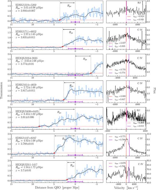
He ii transmission spectra of 7 |$z$| ≃ 4 quasars in our data sample (see Table 1). The blue binned lines show the HST/COS spectra (|$0.24\ {\rm {\mathring{\rm A} }/pixel}$|), while the black lines show the 0.97 Mpc-smoothed He ii transmission, respectively. The magenta error bar illustrates the redshift uncertainty of the corresponding quasar. The values of measured proximity zone sizes are indicated by the red squares, where the smoothed transmission crosses the 10 per cent threshold (red horizontal lines). The panels on the right side show the profiles of C iv and H β lines used to measure the systemic redshift of the corresponding quasar. The flux density is given in units |$10^{-17}\ {\rm erg}\ {\rm s}^{-1}\ {\rm cm}^{-2}\ {\rm {\mathring{\rm A} }}^{-1}$| for all quasars, except HE2QS J2354–2033, for which the flux is given in counts.
The dominant source of uncertainty in our proximity zone measurements results from quasar redshift errors. It is well known that the primary broad rest-frame UV/optical emission lines that are accessible in the optical/near-IR for |$z$| > 3.5 quasars have line centres which can differ from systemic by as much as |${\sim } 3000\, {\rm km\, s^{-1}}$| due to outflowing/inflowing material in the so-called broad line regions of quasars (Gaskell 1982; Tytler & Fan 1992; Vanden Berk et al. 2001; Richards et al. 2002; Shen et al. 2016). To robustly determine systemic redshifts and associated errors for the quasars in our sample, we adopt an approach similar to that described in Shen et al. (2016). The idea is to use a training sample of quasars for which the broad lines in question are present, as well as other features which are known to be good tracers of the systemic frame. For example, Shen et al. (2016) used spectra of |$z$| < 1 quasars taken from Sloan Digital Sky Survey Reverberation Mapping (SDSS-RM) project to determine the relationship between the broad H β λ4861 emission line redshift and systemic redshift determined via Ca ii K λ3934 absorption lines arising from the quasar host galaxy. For cases where the only strong broad far-UV lines like C iv λ1549 are available, as is the case at |$z$| > 3.5 if only optical spectra are available, then one can similarly use a training set to calibrate the relationship between C iv redshifts and those determined from the lower ionization (but still broad) Mg iiλ2798 emission line, which is known to be an excellent tracer of the systemic frame (Shen et al. 2016).
Unfortunately, in case of quasar HE2QS J2354–2033, its redshift appears to be significantly underestimated. From the extent of the He ii proximity zone, we conclude that the C iv emission line of this quasar, which was used to measure the systemic redshift, has a very large blueshift. This is clearly seen in Fig. 1, where the resulting He ii proximity zone has a hugely negative size (Rpz = −3.65 ± 1.68 pMpc). Regrettably, there are no other strong lines in the spectrum of HE2QS J2354–2033 redward of H i Ly α that can be used to accurately determine the redshift of this quasar. Therefore, we exclude the quasar HE2QS J2354–2033 from the subsequent analysis after the initial inspection of the He ii proximity zone, because it cannot provide reasonable constraint on the lifetime.
The redshifts, associated redshift errors, and the emission line used to infer the redshift are given in Table 1. The full details of our procedure, as well as information about the near-IR spectra and the data used for each quasar redshift are provided in Worseck et al. (2018).
3 MODELLING HE ii LY α PROXIMITY ZONES
Our numerical model consists of hydrodynamical simulations and a 1D post-processing radiative transfer algorithm for transport of the ionizing radiation from the quasar through the IGM. In this section, we provide the most important details of our model and refer the reader to the full description given in Khrykin et al. (2016, 2017)
We use the Gadget-3 code (Springel 2005) with simulation box size of 25h−1 comoving Mpc on a side, containing 2 × 5123 particles. Using periodic boundary conditions, we extract 1000 density, velocity, and temperature fields (skewers) drawn in random directions around the most massive haloes (M > 5 × 10¹¹M|$\odot$|) in the outputs of hydrodynamical simulations at |$z$| = 3.7 and |$z$| = 3.9. The resulting skewers have a total length of 160 comoving Mpc with a pixel scale dr = 0.01 comoving Mpc (d|$v$| = 1.0 km s−1).
Extracted skewers are used in our 1D post-processing radiative transfer algorithm based on the C2-Ray code (Mellema et al. 2006), which calculates the evolution of the abundances of e−, H i, He ii, and the gas temperature (Khrykin et al. 2016, 2017). Assuming there is no evolution of cosmic structure between the redshifts of the simulation outputs and that of the corresponding quasars, we simply rescale the gas density of the skewers by a factor (1 + |$z$|)3 to account for cosmological density evolution, where |$z$| is the redshift of the quasar that we are simulating (see Table 1).
There are several important parameters which govern quasar He ii proximity zones: the quasar systemic redshift, the photon production rates Q1Ry and Q4Ry above 1Ry and 4Ry, respectively, the quasar lifetime tQ, and the He ii ionizing background, which sets the value of the initial He ii fraction xHeII, 0, which prevailed in the IGM before the quasar turned on (Khrykin et al. 2016, 2017).1 For each quasar in our data sample, we create a custom set of radiative transfer models based on these parameters. Using their observed i-band magnitudes, we compute Q1Ry and Q4Ry for each quasar in our sample (see Table 1) according to the procedure outlined in Hennawi et al. (2006, see also Section 6). These values, together with the systemic redshift |$z$| are fixed for all radiative transfer models of each individual quasar in our data sample. On the other hand, we explore different combinations of the parameters {tQ, xHeII, 0}. We consider logarithmically spaced quasar lifetime values in the range log10(tQ/Myr) = [ − 2.0, 2.0], with Δlog10(tQ/Myr) = 0.125, whereas the initial He ii fraction can have one of the following values xHeII, 0 = [0.05, 0.10, 0.20, 0.30, 0.50, 0.60, 0.70, 0.90, 1.00]. This results in a grid of 297 radiative transfer models, with 1000 He ii Ly α transmission spectra per model, for each quasar in our data sample.
4 ESTIMATING THE QUASAR LIFETIME AND INITIAL HE ii FRACTION
4.1 Mock He ii spectra and the size of the proximity zone
Following the same procedure applied to the observational data, we smooth our simulated He ii Ly α transmission spectra with a Gaussian with width of 0.97 proper Mpc (see Section 2). Examples of mock He ii transmission spectra smoothed in this way are shown by the black curves in Fig. 2, whereas the blue curves show the original full-resolution mock spectra that results from our modelling procedure. The proximity zone sizes are marked by the red squares. It is apparent from the left-side panels of Fig. 2 that, as expected, the size of the proximity zone increases for longer quasar lifetimes. This dependence of the proximity zone size on quasar lifetime exists because the IGM responds to the changes in the radiation field and attains a new ionization equilibrium state on a finite equilibration time-scale, which is |$t_{\rm eq} \simeq 1 / \Gamma _{\rm bkg}^{\rm HeII} \approx 30$| Myr for He ii at |$z$| ≃ 3–4 (Khrykin et al. 2016). The left-hand panel of Fig. 3 illustrates the dependence of Rpz on quasar lifetime determined from our mock spectra with different lifetimes. It is apparent that for short quasar lifetimes (tQ ≤ teq) the median proximity zone size Rpz grows with lifetime, until tQ becomes larger than the equilibration time (tQ ≥ teq), at which point the median Rpz saturates and stops growing (Khrykin et al. 2016).
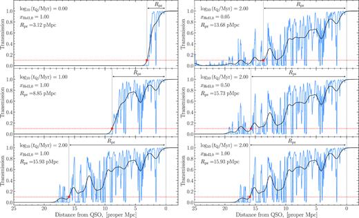
Examples of He ii transmission profiles in our radiative transfer simulations of quasar SDSS J1319+5202 at redshift |$z$| = 3.916 and Q4Ry = 1056.82 s−1 (see Table 1). The left columns show He ii transmission spectra (blue) and smoothed He ii transmission profiles (black) in models with initial He ii fraction xHeII, 0 = 1.00 and three different quasar lifetimes, whereas the right-hand column shows the case of a varying initial He ii fraction, but a fixed quasar lifetime log10(tQ/Myr) = 2.0. The red horizontal lines indicate the 10 per cent transmission threshold, and the corresponding sizes of He ii proximity zones (marked by red squares) are indicated by the black arrows.
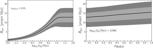
Dependence of the He ii proximity zone size Rpz on quasar lifetime tQ (left-hand panel, with fixed xHeII, 0 = 0.05) and initial He ii fraction xHeII, 0 (right-hand panel with fixed log10(tQ/Myr) = 2.0) in radiative transfer simulations for quasar SDSS J1319+5202. The light and dark grey shaded areas show 1σ and 2σ standard deviations of Rpz, respectively, whereas the solid black line illustrates the median values.
A much weaker increasing trend can be seen in the right-hand panels of Fig. 2 where the Rpz is larger for higher initial He ii fraction. This trend may seem counter-intuitive upon examination of the full-resolution transmission profiles (blue curves), which exhibit more transmission at larger distances from the quasar for lower values of initial He ii fraction. This is because the shape of the transmission profile depends on both the initial He ii fraction which is set by the ionizing background, as well as the amount of photoelectric heating of the IGM resulting from the reionization of He ii, which is known as the thermal proximity effect (see also Bolton, Oh & Furlanetto 2009; Meiksin, Tittley & Brown 2010; Khrykin et al. 2017). The overall increase in transmission at larger radii from the quasar in models with low xHeII, 0 is caused by the higher He ii background as compared to models with xHeII, 0 > 0.50. Khrykin et al. (2016) showed that the effect of He ii background, which sets the value of the initial He ii fraction, on He ii proximity zone becomes prominent at distances where the quasar photoionization rate |$\Gamma _{\rm HeII}^{\rm QSO}$| is no longer the dominant contribution to the total photoionization rate, i.e. |$\Gamma _{\rm HeII}^{\rm QSO} \lesssim \Gamma _{\rm HeII}^{\rm bkg}$|. However, the standard definition of the proximity zone size that we use, which is when the smoothed transmission crosses 10 per cent, is insensitive to the information about |$\Gamma _{\rm HeII}^{\rm bkg}$| encoded in the He ii transmission at the outskirts of the proximity zones. This is because at larger distances, where |$\Gamma _{\rm HeII}^{\rm QSO}$| becomes comparable to the background, the transmission is much lower than 10 per cent, which is visible in the right-hand panels of Fig. 2 (a similar argument explains why the H i Lyα proximity zones of |$z$| ∼ 6 quasars are not good probes of xHI and reionization (Eilers et al. 2017)). On the other hand, the photoionization of He ii by the quasar causes significant heating of the IGM gas. The more singly ionized helium present in the surrounding IGM, the more photoelectric heating results from the absorption of hard photons. Because of the τLyα ∝ T−0.7 temperature dependence of the He ii Ly α optical depth, this heating boosts the transmission in the proximity zone for higher values of xHeII, 0 (Khrykin et al. 2017). Therefore, the smoothed transmission profiles cross the 10 per cent threshold at larger radii in case of higher xHeII, 0 values.
The competition between the increased transmission in the ambient IGM for small xHeII, 0, the 10 per cent transmission threshold being too high to be probed |$\Gamma _{\rm HeII}^{\rm bkg}$|, and the increased transmission due to the thermal proximity effect for higher xHeII, 0 results in an overall weak dependence of proximity zone size with initial He ii fraction, illustrated in the right-hand panel of Fig. 3.
4.2 Distribution of the proximity zone sizes
In general, density fluctuations in the IGM give rise to a broad distribution of proximity zone sizes Rpz for a given set of model parameters (Khrykin et al. 2016), as illustrated in Fig. 3. Furthermore, the uncertainty in quasar redshifts also adds a significant amount of scatter. This is apparent from Table 1 where it is seen (second to last column) that our largest redshift errors, which are those derived from the C iv emission line, result in an uncertainty |$\sigma (R_{\rm pz}) \simeq 1.7\, {\rm Mpc}$|, comparable to the smallest measured proximity zone sizes. Notwithstanding these uncertainties, a comparison of the Rpz distributions from our radiative transfer models to our data sample can still yield constraints on the quasar lifetime. This is readily apparent from inspection of Fig. 4, where we show the observed distribution of Rpz along with the predicted distributions from our simulations for different combinations of model parameters tQ and xHeII. Similar to Fig. 2, the left-hand panel of Fig. 4 shows the distribution of Rpz for models with a fixed initial He ii fraction (xHeII, 0 = 1.00), and three different values of quasar lifetime whereas the right panel shows results at fixed quasar lifetime log10(tQ/Myr) = 0.00 and three different values of xHeII, 0. Each model histogram of simulated He ii proximity zone sizes is derived from 600 mock Rpz measurements – where we take 100 Rpz from the model of each of the six quasars for the corresponding log10(tQ/Myr) and xHeII, 0 values. These model histograms are then normalized to six, which is the total number of quasars in our data sample. We incorporate redshift errors into our simulated distributions of Rpz using the uncertainties on σ(Rpz) reported in Table 1. Specifically, we randomly draw a Gaussian-distributed redshift error using the σ(Rpz) specific to each quasar and add these to the 100 simulated Rpz values for each quasar and each combination of model parameters.
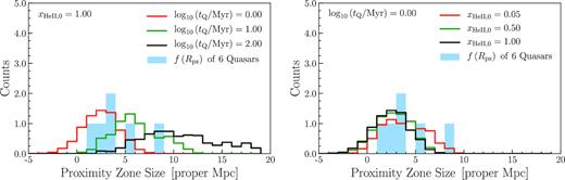
Example of f(Rpz) distributions in radiative transfer simulations. Similar to Fig. 2, the left column illustrates the Rpz distributions in models with varying quasar lifetime and xHeII, 0 = 1.00, whereas the right column shows the case of fixed quasar lifetime at log10(tQ/Myr) = 0.00 and different values of the initial He ii fraction. The blue histogram in both panels illustrates the proximity zone sizes of quasars in our data sample.
Inspection of the left-hand panel of Fig. 4 already reveals that lifetimes around |$t_{\rm Q}\sim 1\, {\rm Myr}$| appear to be preferred by the data. Whereas the right-hand panel clearly indicates the high degree of overlap between the simulated histograms for different values of xHeII. This overlap is a direct result of the weak dependence of Rpz on initial He ii fraction discussed in the previous section (see Fig. 3). This weak sensitivity combined with redshift uncertainties suggests it will be challenging to infer the xHeII, 0 for these quasars. We come back to this question in Section 5.
4.3 Bayesian inference of model parameters
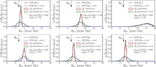
Example kernel density estimation on several distributions of simulated Rpz. The top row illustrates the results for several models with varying quasar lifetimes, and a fixed value of the initial He ii fraction, whereas the bottom row shows similar results, but now for a fixed value of quasar lifetime and different xHeII, 0. The red and green histograms in each panel illustrate the simulated Rpz distributions before and after adding redshift errors. The black and blue curves are the, respective, smooth KDE functions of Rpz. The arrow in each panel indicates the value of Rpz for quasar HE2QS J2311–1417 (see Table 1).
As stated previously, redshift uncertainty constitutes a significant source of error, which would alter the outcome of the parameter inference if neglected. We therefore model the impact of these redshift uncertainties on the Rpz PDF by adding random Gaussian-distributed redshifts errors with standard deviation σ(Rpz) (see Table 1) to the simulated Rpz of each quasar, and perform the KDE on these noisy values. The results are illustrated in Fig. 5, where Rpz distributions with redshift uncertainty (σ(Rpz) = 1.72 pMpc for HE2QSJ2311–1417, see Table 1) included are shown by green histograms, and the corresponding KDEs are illustrated by the blue lines. It is clear that incorporating redshift uncertainties into our Rpz distributions makes them broader and reduces the discriminating power of each individual proximity zone size measurement.
In order to calculate the likelihood of the data for any combination of model parameters, we can then simply evaluate the corresponding KDE PDF at the observed value of Rpz (see Table 1) for the quasar in question. This procedure results in 297 determinations of the likelihood at each location {tQ, xHeII, 0} on our model grid for each quasar. We use bivariate spline interpolation to compute |$\mathscr {L}\left(R_{\rm pz} | t_{\rm Q}, x_{\rm HeII,0} \right)$| for any combination of {tQ, xHeII, 0} between the model grid points in our parameter space.
Armed with the above likelihood, we can now conduct Bayesian inference of model parameters for each quasar using Markov Chain Monte Carlo (MCMC). Given our lack of knowledge about the He ii background, which sets the initial He ii fraction, at the redshifts considered in this work, we choose a flat linear prior on xHeII, 0 from xHeII, 0 = 0.00 to xHeII, 0 = 1.00. On the other hand, we set a flat logarithmic prior on |${\rm log}_{10}\left(t_{\rm Q} / {\rm Myr} \right)$| from −2.0 to 2.0. The lower value of |${\rm log}_{10}\left(t_{\rm Q} / {\rm Myr} \right) =-2.0$| is motivated by the ubiquitous presence of the LOS proximity effect in the H i Ly α forest (but see Eilers et al. 2017), which implies lifetimes in excess of |$t_{\rm Q} \gtrsim 1/ \Gamma _{\rm HI} \simeq 0.01\, {\rm Myr}$| for the vast majority of quasars. The upper value of |${\rm log}_{10}\left(t_{\rm Q} / {\rm Myr} \right)=2.0$| is chosen as it lies in the upper range of lifetime estimates in the literature based on both quasar duty cycle and black hole growth arguments (see Martini 2004, for a review). Furthermore, for tQ in excess of |$100\, {\rm Myr}$|, several of the assumptions that we are making in the modelling, like our neglect of cooling, and our post-processing approach, which implicitly assumes that cosmic structure is fixed over the time-scales that the quasar radiation alters its environment, begin to break down.
We will describe the results of our MCMC inference in the next section, where we will also see that our results are not hugely sensitive to this choice of priors.
5 RESULTS
Given the likelihood of our data, given the model parameters in equation (2), and our interpolation procedure which allows us to evaluate this likelihood at any point in our parameter space {tQ, xHeII, 0}, we now proceed to sample this likelihood with MCMC to determine the posterior distribution of the model parameters for each quasar in the data sample. To this end, we use the publicly available Python MCMC software emcee Foreman-Mackey et al. (2013), which implements an affine-invariant MCMC ensemble sampling algorithm (Goodman & Weare 2010). The results of the MCMC sampling of the posterior distribution of each quasar in our data sample are shown in Fig. 6, where the contours illustrate the 95 (blue) and 68 per cent (red) confidence intervals, respectively. Marginalized posterior probability distributions for each parameter log10(tQ/Myr) and xHeII, 0 are also shown by the histograms. There are several noticeable results and trends that we now discuss.
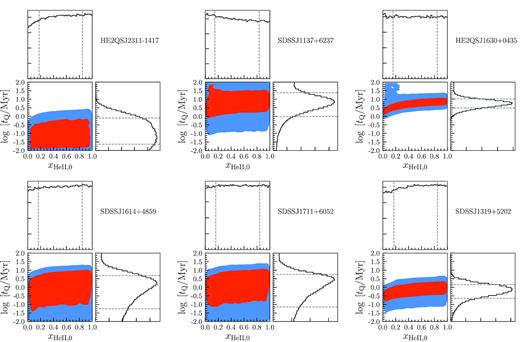
Constraints on the quasar lifetime and the initial He ii fraction from the MCMC analysis of the six quasars in the data sample. The 95 (red) and 68 per cent (blue) confidence levels from the MCMC calculations are shown. The histograms illustrate the corresponding marginalized posterior probability distributions of each parameter.
5.1 Constraints on the initial He ii fraction
We begin with the constraints on the initial He ii fraction. As was previously stated in Section 4.2, the large degree of overlap between the model Rpz distributions for different values of xHeII, 0 and fixed tQ (see Fig. 4), which ultimately results from the very weak dependence of Rpz on xHeII, 0 shown in Fig. 3, suggests that it would be difficult to infer xHeII, 0 with the current data set. This is indeed the case – the broad flat posterior distributions for xHeII, 0 in Fig. 6, which hardly differ from our assumed flat prior, indicate that the data is not very informative and the initial He ii fraction in the ambient IGM surrounding our seven quasars is virtually unconstrained.
5.2 Constraints on the quasar lifetime
Fig. 7 shows the 1D posterior probability distributions for all seven quasars in our sample, marginalized over the initial He ii fraction. It is clear upon inspection of these posteriors that in some cases we are able to measure the quasar lifetime, whereas in others we can only set upper limits. Clearly, this distinction depends upon the strength of the peak in the posterior probability. In order to distinguish between measurements and limits, we use the following criterion. If the maximum value of the marginalized posterior probability distribution is at least four times larger than the larger of the two posterior probability values at the edges of the log10(tQ/Myr) parameter grid, then we classify it as a measurement. In this case, we quote the 50th percentile of the posterior distribution as the measured value, whereas the 16th and 84th percentiles are quoted as our uncertainties. On the other hand, for the flatter posterior probability distributions which do not satisfy the above criteria, we report an upper limit on the quasar lifetime. We choose to quote the 95th percentile value as our upper limit (effectively 2σ) on the lifetime.
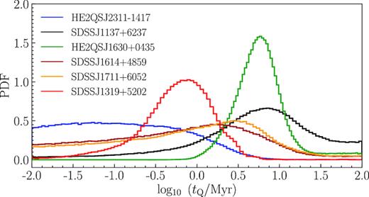
1D posterior probability distributions of log10(tQ/Myr) from MCMC calculations marginalized over the initial He ii fraction. Each histogram represents the results for a quasar in our data sample.
One issue with the upper limits as we define them is that they clearly depend on the range of simulated log10(tQ/Myr) values, i.e. on our choice of a flat logarithmic prior on the quasar lifetime extending from log10(tQ/Myr) = −2.0 to log10(tQ/Myr) = 2.0. However, as was discussed in Section 4.3, the lower limit of our prior is physically motivated observations of the H i LOS proximity effect. The upper limit of our prior is determined by limitations of our modelling procedure, but we see that the proximity zones are all so small that the resulting posteriors are all very small at log10(tQ/Myr) = 2.0, and thus it does not influence our results.
The results of our lifetime inference for all quasars in our data sample are summarized in Table 1, which we discuss further in what follows.
5.2.1 SDSS J1319+5202
The red histogram in Fig. 7 illustrates the marginalized lifetime posterior probability distribution for the quasar SDSS J1319+5202. We infer the lifetime of |${\rm log}_{10} \left(t_{\rm Q} / {\rm Myr}\right) = -0.20^{+0.36}_{-0.45}$|, indicating that this quasar is relatively young. It is also clear from the shape of the posterior that for this case of highly constraining data we are totally insensitive to our choice of priors. The reason we are able to constrain tQ so tightly for SDSS J1319+5202 is that it is the second most luminous object in our sample, which also has the smallest redshift uncertainty σ(Rpz) = 0.98 Mpc as inferred from its Hβ emission line redshift (see Table 1).
Proximity zone sizes Rpz increase with luminosity (Khrykin et al. 2016), implying that the relative error on Rpz should be smallest for the brightest sources. This appears to be reflected in SDSS J1319+5202 which has the third largest proximity zone size of Rpz = 3.62 ± 0.98 Mpc. In contrast with the green histograms (blue curves) in Fig. 5 for HE2QS J2311–1417 which has a |$89{{\ \rm per\ cent}}$| relative error on Rpz, the |$27{{\ \rm per\ cent}}$| relative error on Rpz for SDSS J1319+5202 implies its Rpz PDFs are significantly less broadened by the redshift uncertainty. As a result, the likelihood values, obtained by evaluating the respective KDE (see Section 4.3), are less similar for different tQ models, resulting in higher lifetime precision.
5.2.2 HE2QS J1630+0435
It is apparent from the green histogram in Fig. 7 that the best lifetime constraint we obtain is for the most luminous quasar in the sample HE2QS J1630+0435, which has Rpz = 8.43 ± 1.02 Mpc. From this distribution, we deduce the lifetime to be |${\rm log}_{10} \left(t_{\rm Q} / {\rm Myr}\right) = 0.76^{+0.26}_{-0.28}$|. Similar to SDSS J1319+5202, the redshift error for this quasar translates into a small uncertainty of σ(Rpz) = 1.02 Mpc owing to the H β emission line redshift. This constitutes a ≃12 per cent relative error on Rpz, which allows us to constrain the lifetime with good precision.
5.2.3 SDSS J1137+6237
The black histogram in Fig. 7 shows the marginalized posterior probability distribution for the lifetime of quasar SDSS J1137+6237. This quasar has the second biggest proximity zone (Rpz = 4.92 ± 1.68 Mpc) in our sample. Taking into account its relatively low luminosity, it is possible that it has a long lifetime. However, while this quasar has only |${\approx } 34{{\ \rm per\ cent}}$| relative error on the proximity zone size (comparable to |${\approx } 27{{\ \rm per\ cent}}$| error for SDSS J1319+5202), which, in principle, should provide good constraint on quasar lifetime, the resulting posterior distribution looks different than in case of SDSS J1319+5202 and HE2QS J1630+0435. Namely, the long tail of similar high posterior probabilities at log10(tQ/Myr) > 1.25, that are only ≈2.5 times lower than the peak of the distribution, does not allow us to make a clear measurement of quasar lifetime, according to the criterion defined in Section 5.2.
This decreased constraining power at high-tQ values arises from the fact that sensitivity of Rpz measurements to quasar lifetime is limited by the value of the equilibration time-scale teq (see Section 4.1 for more details), which is teq ≃ 25 Myr at |$z$| ≃ 4. For lifetimes longer than the equilibration time-scale tQ ≳ teq, proximity zone size Rpz saturates and no longer increases with increasing tQ as shown in the left-hand panel of Fig. 3. Consequently, the Rpz PDFs for tQ ≳ teq are comparable, as are the estimated likelihoods of models with tQ ≳ teq. Therefore, our inference cannot distinguish between these models, which results in a tail in the posterior distribution, clearly seen in Fig. 7 for SDSS J1137+6237. Given the shape of its posterior, we can only quote a |$95{{\ \rm per\ cent}}$| lower limit on its lifetime. To this end, we calculate the 5th percentile of the posterior distribution for quasar SDSS J1137+6237, which yields log10(tQ/Myr) > −0.90.
5.2.4 The remaining quasars
It is apparent from Table 1 that for the remaining quasars the uncertainties σ(Rpz) arising from redshift error are a much larger fraction of their proximity zone sizes. The resulting broadening of the model Rpz PDFs (see Fig. 5) results in weaker constraints as illustrated by the flatter less peaked posterior distributions of these quasars in Fig. 7. As a result, following our definition of a measurement versus an upper limit, we can only provide 95 per cent upper limits on tQ for these quasars. Although in one case this limit is particularly strong, namely the small proximity zone Rpz = 1.94 ± 1.72 Mpc of HE2QS J2311–1417, combined with its relatively high luminosity yields a 95 per cent upper limit of log10(tQ/Myr) < 0.31, strongly ruling out long lifetimes >10 Myr.
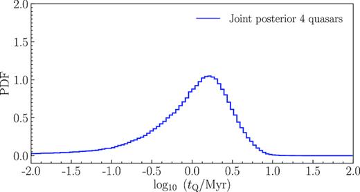
1D posterior probability distribution of log10(tQ/Myr) from joint MCMC calculations of four quasars, marginalized over the initial He ii fraction.
6 DISCUSSION
In this section, we discuss systematics and several assumptions that went into our lifetime estimates and how they are relevant for placing robust constraints on quasar lifetime and initial He ii fraction in the IGM.
6.1 Uncertainties in the photon production rate
We have demonstrated how the radial extent of the He ii proximity zone constrains the quasar lifetime. However, the size of the He ii proximity zone Rpz also depends on the quasar spectral energy distribution (SED, see Khrykin et al. 2016), which we have assumed to be determined perfectly by the apparent magnitudes of the quasars and an assumed spectral slope. In what follows, we discuss how the uncertainties in quasar SED change the constraining power of our method.
First, the slope α4Ry → ∞ determines the number of hard photons, and might affect the thermal and ionization states of IGM in quasar proximity, modifying the resulting He ii transmission profile and value of the Rpz (see Section 4.1). Unfortunately, this slope is currently not determined, and in this work, we have assumed that the same power-law slope α1Ry → ∞ = 1.5 governs the quasar spectrum for photon energies above 1 Ry. However, in Khrykin et al. (2016), we investigated the impact of the variation in the slope α4Ry → ∞ on the resulting He ii transmission profiles. In order to capture the effect of the slope, we fixed the quasar specific luminosity N4Ry, and then freely varied the spectral slope in the range α4Ry → ∞ = 1.1–2.0. We found that due to weak dependence of the quasar He ii photoionization rate on α4Ry → ∞, i.e. |$\Gamma _{\rm HeII}^{\rm QSO} \propto \left(\alpha _{\rm 4Ry \rightarrow \infty } + 3\right)^{-1}$|, the variations in the slope have at most a 10 per cent effect on |$\Gamma _{\rm HeII}^{\rm QSO}$|. Consequently, the resulting He ii transmission profiles are essentially unaffected by these variations (see fig. 12 in Khrykin et al. 2016). For this reason, we conclude that neither the size of the He ii proximity zone Rpz, nor the results of our MCMC inference will change significantly.
On the other hand, variations in the amplitude of the SED, N4Ry, might have a profound effect on inferred values of Rpz and the results of the MCMC inference (Khrykin et al. 2016). We estimate N4Ry for each quasar in the data sample by scaling the observable quasar-specific luminosity N1Ry at the H i ionization threshold of 1 Ry (determined by the corresponding i-band magnitudes and redshifts of the quasars in Table 1) to the He ii ionization threshold with a spectral slope α1Ry → 4Ry (Hennawi et al. 2006; Khrykin et al. 2016). Therefore, the variations of the amplitude N4Ry are inflicted by the uncertainty in α1Ry → 4Ry. Recently, there were several studies that reported although consistent, but slightly different slopes in the extreme-ultraviolet (EUV) at λ ≤ 912Å (Scott et al. 2004; Shull, Stevans & Danforth 2012; Lusso et al. 2015). Our fiducial value α1Ry → 4Ry = 1.5 is slightly harder, but nevertheless consistent with the recent result from Lusso et al. (2015), who found αEUV = 1.7 ± 0.61 (see also Stevans et al. 2014). In what follows, we explore how the uncertainty in α1Ry → 4Ry changes the amplitude of quasar SED and how this affects the results of our inference. To that end, we adopt a much softer slope α1Ry → 4Ry = 2.0, consistent with new measurement by Lusso et al. (2018). We create a new set of radiative transfer models (similar to the discussion in Section 3) for quasar SDSS J1319+5202, and perform the same analysis as in Section 4. Finally, we run the MCMC inference on the resulting Rpz PDFs for α1Ry → 4Ry = 2.0 case.
Fig. 9 shows the resulting posterior probability distribution from the MCMC inference for quasar SDSS J1319+5202 with α1Ry → 4Ry = 2.0, compared to our previous findings (see Fig. 7) with α1Ry → 4Ry = 1.5 . We infer the lifetime |${\rm log}_{10} \left(t_{\rm Q} / {\rm Myr}\right) = 0.17^{+0.39}_{-0.49}$|. It is apparent that the deduced lifetime of SDSS J1319+5202 is ≈0.4 dex longer than what we found in case of a harder spectral slope α1Ry → 4Ry = 1.5 (see Section 5.2).
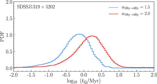
1D posterior probability distributions of log10(tQ/Myr) from MCMC calculations of quasar SDSS J1319+5202 marginalized over the initial He ii fraction. The blue histogram shows the results of the inference performed on radiative transfer simulations with quasar spectral slope between 1 Ry and 4 Ry set to our fiducial value α1Ry → 4Ry = 1.5 (same as in Fig. 7), whereas the red histogram illustrates the results for modified slope α1Ry → 4Ry = 2.0 (see discussion in the text for more details).
6.2 Comparison to other constraints on quasar lifetime
Our study of six |$z$| ∼ 4 quasars suggests lifetimes of order tQ ≃ 1 Myr. In what follows, we discuss these results in the context of recent quasar lifetime measurements at |$z$| ∼ 6, and their implications for the evolution of SMBH in the high-|$z$| Universe.
Eilers et al. (2017) analysed the H i proximity effect in the spectra of 34 |$z$| ≃ 6 quasars and reported the discovery of three objects with exceptionally small H i proximity zones that imply lifetimes tQ ≲ 0.1 Myr, with one particular quasar shining for only tQ ≲ 0.01 Myr (Eilers et al. 2018). These findings essentially constrain the fraction of young (tQ ≲ 0.01 Myr) quasars to be 3 per cent. Moreover, Davies et al. in prep reported the upper limit on the total duty cycle of the most distant ULAS J1342+0928 quasar (|$z$| = 7.54; Bañados et al. 2018) to be tQ ≲ 5.4 Myr, based on the IGM damping wing analysis. Consider a simple light bulb light curve model, in which the quasar is assumed to emit at constant luminosity for its entire lifetime tQ. If one randomly samples such light curves with tQ ≃ 1 Myr as suggested by our measurements, the probability of finding quasars that are as young as tQ ≲ 0.01 Myr is 1 per cent, which is consistent with the ≈3 per cent young fraction determined by Eilers et al. (2017) given their statistical error on one object, suggesting that our results are in broad agreement with their discovery of young quasars.
However, such short lifetimes tQ ∼ 1 Myr may be problematic given the constraints from quasar clustering and current theories about how SMBHs grow. Indeed, if one assumes a light bulb model for the quasar light curve, then under this assumption the lifetime tQ and the duty cycle tdc are equivalent, and thus we measure the duty cycle as well. In this case, our findings appear to be at odds with the high values of tdc implied by the strong clustering quasars at |$z$| ≃ 4 measured by Shen et al. (2007). For instance, White et al. (2008) modelled the Shen et al. (2007) clustering strength and found tdc ≃ 1 Gyr, but argued that these long duty cycles are not unexpected from the standpoint of black hole growth given a Salpeter time of |$t_{\rm S}\simeq 180\, {\rm Myr}$| (for Eddington ratios |$L_{\rm bol}/ L_{\rm Edd}\simeq 0.25$|; Kollmeier et al. 2006). However, White et al. (2008) also argued that the dispersion σ in the relationship between quasar luminosity L and dark matter halo mass Mhalo must then be less than 50 per cent (99 per cent confidence) for this high tdc. A decrease in duty cycle to tdc ≃ 100 Myr would already require an unphysically small amount of scatter σ ≲ 10 per cent in the L − Mhalo relation. Thus, if our quasars emit their radiation in one continuous episode such that |$t_{\rm Q} = t_{\rm dc} \sim 1\, {\rm Myr}$|, there appears to be no easy way to reconcile our results with the clustering measurements. Furthermore, for our short inferred lifetimes and the assumption of a simple light curve, it would be impossible to grow |${\sim } 10^9\, M_{\odot }$| black holes in these quasar hosts without invoking super-Eddington accretion rates (Davies et al in prep.).
One way to solve this problem would be to invoke a so-called flickering light curve model instead of a light bulb one (Ciotti & Ostriker 2001; Novak et al. 2011; Oppenheimer & Schaye 2013). In this picture, the ultraviolet continuum emission from the quasar fluctuates as a result of either intrinsic changes in the accretion flow, or time variable obscuration along our line-of-sight. In general, the response of proximity zones to flickering light curves depends on the details of the light curve shape and the ionization state of the ambient IGM around the quasar. But the key point is that it takes the IGM an equilibration time-scale |$t_{\rm eq} \simeq 1/ \Gamma _{\rm bkg}^{\rm HeII}$| to respond to changes in the radiation field. For the sake of illustration, consider a toy model light curve whereby quasars emit continuously as light bulbs for |$t_{\rm on} = 1\, {\rm Myr}$|, but are then quenched for |$t_{\rm off} = 10\, {\rm Myr}$|, and that this on/off behaviour continues over a Hubble time tH. If He ii in the IGM is highly ionized, then because toff is comparable to the equilibration time |$t_{\rm eq} \simeq 30\, {\rm Myr}$|, gas in the IGM has enough time to recombine to ambient IGM ionization levels during the off periods. As a result, the lifetimes we would infer from studying the proximity zones of active quasars would be tQ ≃ ton, which however grossly underestimates the duty cycle |$t_{\rm dc} = (t_{\rm on}/ t_{\rm off})t_{\rm H} = 160\, {\rm Myr}$| at |$z$| ∼ 4. This toy model suggests that one can find a flickering light curve model which can satisfy our proximity zone constraints and still provide a sufficiently long duty cycle |$t_{\rm dc}\sim 100\, {\rm Myr}$| required to grow the SMBH and closer to the values deduced from clustering. Although we note that the |$z$| ∼ 4 quasar clustering results appear to tightly constrain the allowed light curves, since according to White et al. (2008) |$t_{\rm dc}\sim 100\, {\rm Myr}$| would start to imply an unphysically small amount of scatter σ in the relationship between quasar luminosity and and dark matter halo mass. More careful modelling of flickering light curves is clearly an interesting subject for future work.
7 CONCLUSIONS
We have measured the He ii proximity zone sizes in the spectra of six |$z$| ∼ 4 quasars. We performed cosmological hydrodynamical simulations, post-processed with 1D radiative transfer algorithm to analyse these He ii proximity zones. We have used a fully Bayesian MCMC formalism to compare the distribution of He ii proximity zone sizes in simulations to the sizes of observed proximity zones in order to infer the quasar lifetimes, as well as the initial He ii fraction in the IGM surrounding these quasars.
Our simulations indicate that proximity zone sizes are relatively insensitive to the He ii fraction of the ambient IGM surrounding the quasars, which is confirmed by the results of our inference. We thus marginalize over the unknown xHeII to obtain constraints on quasar lifetime. We inferred |${\rm log}_{10} \left(t_{\rm Q} / {\rm Myr}\right) = -0.20^{+0.36}_{-0.45}$| for quasar SDSS J1319+5202 and |${\rm log}_{10} \left(t_{\rm Q} / {\rm Myr}\right) = 0.76^{+0.26}_{-0.28}$| for the HE2QS J1630+0435, but were able to put only 95 per cent limits on the lifetime of the remaining quasars due to large uncertainties in their systemic redshifts. In order to mitigate the effect of redshift error, we have also performed a joint analysis on four quasars and find |$\langle {\rm log}_{10} \left(t_{\rm Q} / {\rm Myr}\right) \rangle = 0.07^{+0.40}_{-0.55}$|, which is consistent with the two other measurements. All of our results thus seem to point to quasar lifetimes of tQ ∼ 1 Myr at |$z$| ∼ 4. We discussed this result in the context of other lifetime estimates at |$z$| ≳ 6 that seem to deduce a comparable value, as well as the implication from quasar clustering that the duty cycles of |$z$| ∼ 4 quasars are much longer.
Unfortunately, the large uncertainties inherent in using broad emission lines in the rest-frame UV/optical to determine quasar redshifts significantly limit the precision with which we can measure the lifetimes of individual quasars. An important direction for the future would be to obtain accurate systemic redshifts of these and other He ii quasars via mm and sub-mm observations of CO and [C ii] 158 μm lines arising from cool gas reservoirs in the quasar host galaxies. Indeed, the much smaller systemic redshift errors (|${\sim } 50\, {\rm km\, s^{-1}}$|) would enable lifetime measurements for all of the quasars considered here with a much smaller error of ∼0.10 dex. We also note that a large sample of ∼20 He ii Ly α forest spectra exists at |$z$| ∼ 3, and besides significantly improved statistics one also benefits from much better constraints on the He ii fraction of the ambient IGM. We emphasize that the statistical techniques presented in this paper can also be applied to the measurements of quasar lifetime from the H i proximity effect at |$z$| ∼ 6 (Eilers et al. 2018, Davies et al in prep). Furthermore, it would be interesting to explore statistical methods (for both He ii and H i proximity zones) which uses the entire transmission profile (Davies et al. 2018) instead of just Rpz. Finally, it would be interesting to perform a joint analysis of the line-of-sight He ii proximity effect and the thermal proximity effect (resulting from He ii photoelectric heating) in the H i Lyα forest (Khrykin et al. 2017) at |$z$| ≃ 4, which will provide additional constraining power (especially for determining xHeII, 0) as well as an independent check of our results.
ACKNOWLEDGEMENTS
The authors thank Matt McQuinn, Frederick Davies, Christina Eilers, Hector Hiss, Michael Walther, and Tobias Schmidt for useful discussions. We are grateful to the anonymous referee for comments and suggestions. ISK acknowledges support from the grants of the Russian Foundation for Basic Research (RFBR) No. 18-32-00798 and No. 17-52-45063, and partial support from the grant of the Ministry for Education and Science of the Russian Federation (3.858.2017/4.6). GW acknowledges support by the Deutsches Zentrum für Luft- und Raumfahrt (DLR) grant 50OR1720. Partly based on observations made with the National Aeronautics and Space Administration (NASA)/European Space Agency (ESA) Hubble Space Telescope, obtained at the Space Telescope Science Institute, which is operated by the Association of Universities for Research in Astronomy (AURA), Inc., under NASA contract NAS 5-26555. Support for this work was provided by NASA through grant number HST-AR-15014.003-A from the Space Telescope Science Institute, which is operated by AURA, Inc., under NASA contract NAS 5-26555. These observations are associated with Programs 13013, 13875, and 14809. Archival Hubble Space Telescope data (Program 12249) were obtained from the Mikulski Archive for Space Telescopes (MAST).
Footnotes
In what follows, we quote the values of initial He ii fraction that correspond to the adopted values of the He ii background in the radiative transfer simulations
