


Abstract
We investigate the clustering properties and close neighbour counts for galaxies with different types of bulges and stellar masses. We select samples of ‘classical’ and ‘pseudo’ bulges, as well as ‘bulge-less’ pure disc galaxies, based on the bulge/disc decomposition catalogue of SDSS galaxies provided by Simard et al. (2011). For a given galaxy sample we estimate: the projected two-point cross-correlation function with respect to a spectroscopic reference sample, |$w$|p(rp), and the average background-subtracted neighbour count within a projected separation using a photometric reference sample, Nneighbour(< rp). We compare the results with the measurements of control samples matched in colour, concentration, and redshift. We find that, when limited to a certain stellar mass range and matched in colour and concentration, all the samples present similar clustering amplitudes and neighbour counts on scales above |${\sim }0.1\, h^{-1}$| Mpc. This indicates that neither the presence of a central bulge, nor the bulge type is related to intermediate-to-large scale environments. On smaller scales, in contrast, pseudo-bulge and pure-disc galaxies similarly show strong excess in close neighbour count when compared to control galaxies, at all masses probed. For classical bulges, small-scale excess is also observed but only for |$M_{\mathrm{ stars}}\lt 10^{10}\, \mathrm{M}_\odot$|; at higher masses, their neighbour counts are similar to that of control galaxies at all scales. These results imply strong connections between galactic bulges and galaxy–galaxy interactions in the local Universe, although it is unclear how they are physically linked in the current theory of galaxy formation.
1 INTRODUCTION
A bulge is a commonly existing central component of a spiral galaxy that has more concentrated light and stars compared to the more extended disc (Sandage 1961). In fact, a prominent bulge component is observed in at least half of the bright spiral galaxies with stellar mass greater than |${\sim }10^9\, \mathrm{M}_{\odot }$| (Fisher & Drory 2011). Bulges can be divided into two different subcategories: classical bulges which have similar properties as elliptical galaxies, and pseudo-bulges which are more like spiral galaxies, being bluer, more discy, more rotation dominated and more active in terms of star formation (Kormendy & Kennicutt 2004). In some studies, pseudo-bulges have been further divided into flat ‘discy pseudo-bulges’ and thick ‘boxy/peanut bulges’, depending on the structure of the central components (Athanassoula 2005). In many cases, different types of bulges have been found to coexist in the same galaxy. The fraction of composite bulges in barred galaxies can be as high as 70 per cent (Méndez-Abreu et al. 2014).
Three physical processes have been proposed for the formation and growth of galactic bulges. The first process is galaxy merging, during which materials of two or more galaxies condense into the centre of a galaxy (Aguerri, Balcells & Peletier 2001; Hammer et al. 2005). Another process that could form bulge in a relative short time-scale is the collapse and formation of bulges due to clumpy disc instability (Noguchi 1999; Elmegreen, Bournaud & Elmegreen 2008). The third one is secular evolution of slow growth of bulges, due to bar-induced disc instability (Kormendy & Kennicutt 2004; Athanassoula 2005).
In general, the current theoretical picture is that classical bulges are produced during rapid processes like merger and clumpy disc instabilities which happen more often at high redshifts. On the other hand, secular evolution affects in a long term the appearance and growth of pseudo-bulges, and is still shaping morphologies of galaxies at the present day (Obreja et al. 2013; Laurikainen, Peletier & Gadotti 2016). Detailed studies of the formation of bulges also indicate possibilities beyond this general picture. For example, mergers as well as external accretion of gas could also lead to the formation and growth of pseudo-bulges (Eliche-Moral et al. 2013; Guedes et al. 2013; Querejeta et al. 2015; Sauvaget et al. 2018), while wet major mergers could produce a disc galaxy with both classical bulge and pseudo-bulge (Athanassoula et al. 2016). On the other hand, secular evolution can build up some massive bulges in the early universe, without the help of major mergers (Genzel et al. 2008).
Nevertheless, the current picture cannot fully explain the observational properties of bulges. In particular, many giant galaxies have been observed to have no sign of a classical bulge, a result that is inconsistent with the hierarchical clustering cosmology which predicts the opposite, indicating that bulge formation may be somehow suppressed in mergers (Laurikainen et al. 2016). This problem is a strong function of environment: while most of the giant galaxies in the Local Group are bulgeless or with pseudo-bulges, galaxies in Virgo cluster are mostly ellipticals or with classical bulges. In order to loose the tension, minor mergers have been proposed, as an important channel particularly responsible for the formation of pseudo-bulges (e.g. Eliche-Moral et al. 2013), without destroying the existing thin disc in galaxies (e.g. Moster et al. 2010). However, there has been little observational evidence in support of this picture. In fact, very few pseudo-bulge galaxies show signs of tidal interactions of minor mergers (Kormendy & Kennicutt 2004).
While mergers happen more often in denser environment where galaxies have more companions, merger-induced bulges might cluster more strongly than bulges formed through internal processes. In this work, we use the SDSS decomposition catalogue provided by Simard et al. (2011) to select observed galaxies with different morphologies, and compare their clustering properties. We also obtain neighbour counts of these selected galaxy samples, to study their small-scale environment. By examining these statistical properties, rather than looking into galaxies for possible merger indicators (e.g. López-Corredoira & Kroupa 2016) or studying the detailed environment of bulge galaxies (e.g. Henkel et al. 2017; Mishra, Wadadekar & Barway 2017a), we hope to understand further the role merger and environment play in the formation of different types of galactic bulges.
The paper is organized as follows. In Section 2.1, we introduce briefly the Simard et al. decomposition catalogue, and how we select galaxies of different morphologies from it. Methods of measuring galaxy correlation functions and close neighbour counts are described in Section 2.2. In Section 3, we first show clustering results of different types of galaxies in four stellar mass bins, then both clustering and close neighbour count results of matched samples that have the same distributions in redshift, colour, and concentration. Discussions and conclusions are presented in Sections 4 and 5, respectively.
2 DATA AND METHODOLOGY
2.1 SDSS galaxy samples
In this work, we make use of the SDSS galaxy catalogue of Simard et al. (2011) to select samples of classical and pseudo-bulges. Simard et al. (2011) performed a two-dimensional photometric decomposition of bulge and disc components, with the point spread function being convolved, for over a million galaxies in the SDSS Data Release 7 (DR7; Abazajian et al. 2009). Three different fitting models were applied to each galaxy: a pure Sersic profile, a two-component model consisting of a Sersic profile for the bulge and an exponential profile for the disc, and the same two-component model except that the Sersic index nb is fixed to nb = 4. Detailed fitting methods can be found in Simard et al. (2011), as well as some examples of fitting results (their figs 5 and 6). To quantify the robustness of the model fitting, two F-test probabilities are provided: (1) PpS: the probability that the two-component model with a free Sersic index nb is not required compared to a pure Sersic model, and (2) Pn4: the probability that the two-component model with a free nb is not required compared to the two-component model with a fixed index of nb = 4. Simard et al. (2011) showed that, a system truly consisting of both bulge and disc components can be robustly identified by requiring PpS ≤ 0.32. In their catalogue 26 per cent galaxies meet this requirement. However, a Sersic index nb is robustly determined only for 9 per cent of the bulge + disc systems, for which Pn4 ≤ 0.32 is required. Nevertheless, given the large size of the parent catalogue, we are able to select samples of galaxies with well classified bulge types, which are substantially large for our purpose.
We start with all the galaxies in the Simard et al. (2011) catalogue with spectroscopically measured redshifts available from SDSS/DR7. This forms our parent sample, consisting of 692292 galaxies, from which we construct a number of subsamples according to the presence of a bulge and/or the bulge type. First, we select two subsamples of galaxies, with either a ‘pseudo-bulge’ or a ‘classic bulge’ in their centre. For this purpose, following Simard et al. (2011), we first select galaxies with PpS ≤ 0.32 and Pn4 ≤ 0.32, which are expected to be truly a two-component system consisting of an exponential disc plus a bulge with a free index parameter of nb. We further divide these galaxies into two subcatagories, with a bulge type of ‘pseudo’ or ‘classic’, according to the empirical divider of nb = 2 (Kormendy & Kennicutt 2004). Pseudo-bulges are selected to have nb < 2, and classical bulges are the ones with nb > 3. Galaxies with nb = [2, 3] are not considered in order to minimize uncertainty in the classification. Studies of nearby bulge-disc galaxies showed that around 90 per cent of classical (pseudo) bulges have nb > 2 (nb < 2) (figure 1.3 of Fisher & Drory 2016). With less than ∼10 per cent contamination, we expect the statistical results like clustering and neighbour count as we study in this work not to be strongly biased. On the other hand, although a combination of several criteria may be useful to select out the most typical bulge samples, it would decrease the numbers of samples by a large fraction.
In addition, we select the galaxies with Pn4 ≥ 0.68 as the third subsample. These galaxies also have two components, a disc plus a bulge, but the bulge component is better fitted when the Sersic index is fixed to nb = 4. Therefore, these galaxies are also in the class of classical bulge, but are not included in the classical bulge sample with Pn4 ≤ 0.32 and a free nb as defined above.
For comparison, we also select bulge-less pure disc galaxies and elliptical galaxies from the same parent catalogue. Galaxies with PpS ≥ 0.68 are the ones better fitted by a pure Sersic model than a bulge + disc model, and are considered as either a pure disc galaxy or an elliptical galaxy. We then divide the two types according to best-fitting Sersic index, requiring a pure disc to have ng < 2 and an elliptical to have ng > 3. Galaxies with an intermediate ng are not considered for the same reason as above.
The allowed range of Sersic index n (nb for pseudo-bulge and classical bulge, and ng for pure disc and elliptical) in the Simard et al. (2011) sample is 0.5 < n < 8. Following Mishra, Barway & Wadadekar (2017b), we exclude galaxies with n ≥ 7.95 in our samples, since high values of Sersic indices may be associated with fitting problems (Meert, Vikram & Bernardi 2015). Mishra et al. (2017b) also exclude galaxies that have error of n greater than +1σ of error distribution, and exclude galaxies that host a bar when selecting pseudo-bulges. We have checked that when removing galaxies with large errors in n, the results remain similar as when including them. We therefore do not exclude these galaxies to get better statistics. The distributions of error in n as a function of n value in our samples are presented in Appendix A. We also check the effect of galaxies having bars on the determination of Sersic index in Appendix A.
Apart from the commonly used Sersic index criterion (Kormendy & Kennicutt 2004; Fisher & Drory 2008) to select pseudo-bulge and classical bulge as we do in this work, galaxies with different types of bulges also have statistically difference on some other properties (a complete list of properties that define bulge types can be found in Kormendy 2016). In some studies to define galaxies with bulges (e.g. Vaghmare et al. 2015; Mishra et al. 2017b), positions on the Kormendy diagram (Kormendy 1977) and velocity dispersion are also used to select the purest pseudo-bulge sample. In our work, while we aim to get better statistics for both classical and pseudo-bulge galaxies, our pseudo-bulges sample selected based only on Sersic index is not necessarily made of the purest pseudo-bulges as in Vaghmare et al. (2015) and Mishra et al. (2017b). In Appendix B, we discuss and check these additional criteria for galaxies in our selected samples, and test the effect of including them on our results.
We check the robustness of our identification of pure disc and elliptical samples by cross-matching our samples with the morphology catalogues of Nair & Abraham (2010) and Paul, Virag & Shamir (2018). In the matched galaxies, 97.6 (74.0) per cent of our pure discs (ellipticals) have probability of being spiral (elliptical) greater than 0.5 in Paul et al. (2018). 85.9 (86.7) per cent of our pure discs (ellipticals) have types later (earlier) than S0 in Nair & Abraham (2010). Our type determinations of pure discs and ellipticals are largely consistent with these samples of more detailed morphology classification.
In summary, we have selected five samples: three samples for galaxies with different types of bulges, one for pure-disc galaxies, and one for elliptical galaxies. Table 1 lists the name, the selection criteria, and the size of all the samples. Since the number of galaxies in Classical B is relatively small for calculating correlation functions, in the following section we do not analyse Classical B individually, but rather work on a combined sample of Classical A and Classical B, which is referred to as Classical A + B.
Samples of galaxies with different morphologies and bulge types selected from the Simard et al. (2011) catalogue.
| Sample | Selection criteria | Size |
|---|---|---|
| Pseudo-bulge | PpS ≤ 0.32, Pn4 ≤ 0.32, nb < 2 | 19 813 |
| Classical bulge A | PpS ≤ 0.32, Pn4 ≤ 0.32, 3 < nb < 7.95 | 15 906 |
| Classical bulge B | PpS ≤ 0.32, Pn4 ≥ 0.68, nb = 4 | 7219 |
| Pure disc | PpS ≥ 0.68, ng < 2 | 11 102 |
| Elliptical | PpS ≥ 0.68, 3 < ng < 7.95 | 990 |
Fig. 1 displays the distributions of redshift, stellar mass, g − r colour and the concentration parameter for our samples. Stellar masses are taken from the MPA-JHU SDSS catalogue.1 The concentration parameter is defined as the ratio of two radii, enclosing 90 and 50 per cent of the galaxy light in the r band (see Stoughton et al. 2002). Compared with the whole sample without selection of galaxy morphologies as shown in black dotted lines, the galaxies selected in our samples have in general lower redshifts, which can be understood from the fact that closer galaxies are better determined in morphology type. Pure disc galaxies peak at low stellar mass, blue colour, and low concentration, while ellipticals peak on the opposite ends. As expected, pseudo-bulge galaxies are similar to pure disc galaxies in distributions of stellar mass and colour, while galaxies with classical bulges are more like ellipticals in these properties. The distributions of bulge galaxies in concentration, however, are much wider than that of pure disc/elliptical galaxies, showing a relative flat trend in a large range of concentration.
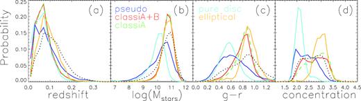
Statistics of the three selected samples (colour lines as labelled). From left to right, panels show distributions of: (a) redshift; (b) stellar mass; (c) petrosian magnitude g–r colour; and (d) concentration. Black dotted lines are the distributions of galaxy properties in the whole sample, without any selection of morphology.
Comparing pseudo-bulge galaxies with classical bulge galaxies, we find the former to be generally less massive, bluer, and less concentrated. Different bulge types show quite a large overlap in colour and concentration space, indicating that these properties cannot be simply used as criteria to distinguish classical bulges from pseudo-bulges.
2.2 Methodology
2.2.1 Two-point cross-correlation functions
In this work, we use two-point cross-correlation function (2PCCF) to quantify the clustering of our galaxies. Below we describe briefly the methodology of measuring the 2PCCF. Detailed description can be found in Li et al. (2006a,b, 2012).
For a given galaxy sample Q, the 2PCCF is measured with respect to a reference galaxy sample G, which is a magnitude-limited galaxy catalogue selected from the SDSS/DR7-based NYU-VAGC catalogue dr72, consisting of about half a million galaxies with r-band Petrosian apparent magnitude limited to r < 17.6, r-band absolute magnitude in the range of |$-24 \lt M^{0.1}_r \lt -16$|, and spectroscopically measured redshift in the range of 0.01 < |$z$| < 0.5. Both r and |$M^{0.1}_r$| are corrected for Galactic extinction, and |$M^{0.1}_r$| is also corrected for evolution and K-corrected to its value at |$z$| = 0.1. The NYU-VAGC catalogue is publicly available,2 and described in detail in Blanton et al. (2005) and Blanton & Roweis (2007). We have constructed a random sample R, which has the same selection effects as, but 10 times larger than the reference sample, following the method described in Li et al. (2006a).
2.2.2 Close neighbour counts
In addition to 2PCCFs, we count the number of companion galaxies in the vicinity of the galaxies in our samples, using a photometric reference sample which is also constructed from the NYU-VAGC version dr72 by selecting galaxies with r-band apparent magnitude down to r < 21. The photometric reference sample includes about 2.5 million galaxies over the same sky area of the galaxy samples being studied. We make a statistical correction for the effect of chance projections on the neighbour counts, by subtracting the average count at the same scale around a large number of randomly placed galaxies. When compared to 2PCCFs, close neighbour counts are not affected by fiber collisions on small scales, and can include much fainter companion galaxies thanks to the photometric sample which is much deeper than the spectroscopic sample, thus probing the effect of close companions over a broader range of mass ratios. Detailed description of the method of estimating close neighbour counts, as well as tests and example applications can be found in Li et al. (2008a,b).
3 RESULTS
3.1 Joint dependence of clustering on galaxy mass and morphology
Galaxy clustering depends on stellar mass, with more massive galaxies being clustered more strongly (Li et al. 2006a). Therefore, we first divide galaxies in each of our samples into four intervals of stellar mass, and estimate the 2PCCF |$w$|p(rp) for each of them. For each of the stellar mass interval, Fig. 2 compares the |$w$|p(rp) measurements for galaxies of different morphological types. The bottom panels in the same figure display the ratios of the |$w$|p(rp) measured from our samples relative to the |$w$|p(rp) measured for all the galaxies in the same stellar mass range as selected from the whole sample of Simard et al. (2011).
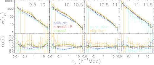
Upper panels: clustering of galaxies in different stellar mass bins, indicated in range of log(Mstars/M⊙) in black. Blue, red, green, cyan, and gold lines are results of pseudo, classical A, classical A + B, pure disc, and elliptical samples, respectively. Black dots are results of the whole Simard et al. sample, matched with the same stellar mass criterion. Bottom panels: for given stellar mass bin, the ratio between 2PCCF of galaxies in selected morphology samples and that of galaxies in the whole sample.
Overall, the figure shows that all the samples appear to cluster similarly at both smallest scales (|$r_\mathrm{ p}\lesssim 0.1 \, h^{-1}$| kpc) and scales larger than a few Mpc. At intermediate scales, different samples show different clustering behaviours. First, galaxies with classical bulges present stronger clustering than those with pseudo-bulges, with larger differences at lower masses, and the difference becomes indistinguishable when stellar mass exceeds |$10^{11} \, \mathrm{M}_{\odot }$|. Secondly, although the error bars are large for the pure disc and elliptical galaxies due to small sample sizes, there is still an obvious trend that pure disc galaxies show weakest clustering and ellipticals appear to cluster most strongly, in a given stellar mass range. It is interesting that galaxies with pseudo-bulges seem to show very similar clustering behaviours to the pure disc galaxies of similar mass, while galaxies with classical bulges are more like ellipticals in terms of mass dependence of clustering. Finally, when compared to the whole sample, the pseudo-bulges are clustered more weakly at all masses except the highest mass bin, while the clustering amplitude of classical bulges is comparable to that of the whole sample at all masses except the lowest masses at which the classical bulges are more strongly clustered.
Previous studies have well established that, at given stellar mass, galaxy clustering depends also on other properties, such as colour and structural parameters, with stronger clustering for galaxies with redder colours and more centrally concentrated light distributions (e.g. Li et al. 2006a). In order to exclude the effect of such residual dependence, for a certain stellar mass bin, we have trimmed the galaxy samples in such a way that they have the same distributions in g − r colour, concentration parameter, and redshift. From what follows we will not consider the elliptical galaxy sample which is too small after trimmed to allow any meaningful statistics. As mentioned above, we will combine the two bulge samples ‘classical A’ and ‘classical B’ into a single sample in order for better statistics. We note that we have repeated all the following analyses using the sample of ‘classical bulge A’ alone, finding pretty much the same results as what we find from the merged sample. Fig. 3 shows the distributions of redshift, g − r and concentration for the three samples: ‘pseudo-bulge’, ‘classical bulge’, and ‘pure disc’, after they are trimmed. At given stellar mass, the three samples are matched very well in all these parameters.
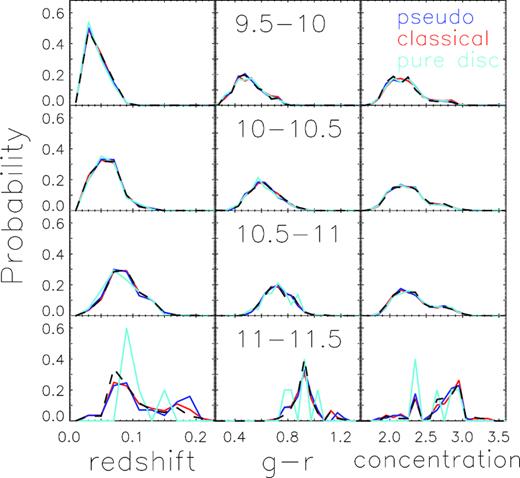
For four stellar mass bins as indicated in range of log(Mstars/M⊙) in black, panels in each row show at the given stellar mass bin, the distributions of redshift, colour, and concentration of galaxies in matched samples. Black dashed lines are distributions of the corresponding control samples.
For each given stellar mass bin, we have constructed a set of 20 control samples to be compared with the three matched samples. The control samples are randomly selected from the reference sample G as mentioned in Section 2.2.1, each required to have the same distributions in redshift, colour, and concentration as the galaxy samples. The number of galaxies included in each control sample is the same as the largest of the matched samples in the stellar mass bin considered. The distributions of redshift, colour, and concentration for the control samples are plotted as black dashed lines in Fig. 3.
The clustering results of the matched galaxy samples and control samples in different stellar mass bins are shown in Fig. 4. For control samples, the median of the 20 control samples is shown as black circles. Ratios of the 2PCCF of the three matched samples relative to the corresponding control samples (black circles) are presented in the lower panels. In general, the differences between different morphology samples and control samples are small, mostly within error bars, except for the most massive bin. Therefore, the significant differences between classical bulge galaxies and pseudo-bulge/pure disc galaxies as seen in Fig. 2 should be largely attributed to their different distributions of redshift, colour, and concentration. For the most massive bin, there seems to have a trend that both pure disc galaxies and pseudo-bulge galaxies cluster less strongly than classical bulge galaxies and the control samples. We would not overemphasize this trend; however, given the large errors in the mass bin.
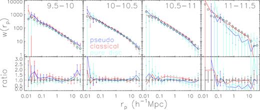
Clustering of galaxies in four stellar mass bins, for galaxy samples matched with the same distributions of redshift, colour, and concentration in given stellar mass bin. The stellar mass intervals are indicated in range of log(Mstars/M⊙) in black. For each stellar mass interval, upper panel gives 2PCCF clustering results of pseudo-bulge galaxies (blue line), classical A + B bulge galaxies (red lines), and pure disc galaxies (cyan lines). Black circles are the median result of the 20 control samples constructed. Error bars on matched galaxy samples are bootstrap errors. The corresponding lower panel shows the ratios between 2PCCF of selected galaxy samples and that of the control sample. Black error bars indicate the 68 percentile distributions of the 20 control samples constructed.
We note that, at smallest scales with |$r_\mathrm{ p}\lesssim 0.1 \, h^{-1}$| Mpc and in some stellar mass bins, both the pure disc galaxies and the pseudo-bulge galaxies tend to present a sharply increasing |$w$|p(rp) when compared to the control samples. However, considering both the small number of pair counts at these small scales and the possible residual effect of SDSS fiber collisions, we are unable to make any firm conclusions based on the |$w$|p(rp) measurements at these scales. In the next subsection, we will focus on these small scales by estimating close neighbour counts. To summarize the analyses presented in this subsection, we have found no significant differences in clustering at scales above |$0.1 \, h^{-1}$| Mpc for all the samples considered in our study.
3.2 Probing the small-scale environment by counting close neighbours
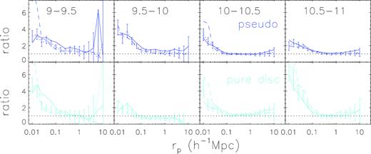
We have estimated the background-subtracted close neighbour count as a function of projected radius, Nneighbour(< rp), in the vicinity of both the samples of different morphology types and the corresponding control samples, using the photometric reference sample down to a given limiting magnitude of rlim as described in Section 2.2.2. Fig. 5 displays the results obtained with rlim = 20, separately for the different stellar mass bins. In a given stellar mass bin, all the samples including the samples of pseudo-bulge, classical bulge, and pure disc galaxies, as well as the control samples, are closely matched in g − r colour, concentration, and redshift as in the previous subsection. First of all, we see that when the stellar mass is limited to a certain range, the neighbour counts at scales larger than |${\sim }0.1 \, h^{-1}$| Mpc for all the samples agree within errors, which are too large to deduce any trend. This is well consistent with the 2PCCF comparison results as presented above.
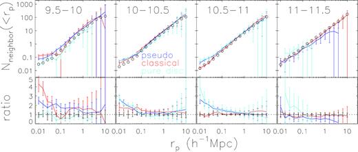
Neighbour counts of galaxies in four stellar mass bins indicated in range of log(Mstars/M⊙) in black, for galaxy samples matched with the same distributions of redshift, colour, and concentration in each panel. Upper panels are the average counts of galaxies in the photometric sample to an r-band limiting magnitude of rlim = 20 within a given projected radius rp from the selected galaxies. Blue/red solid line gives result of pseudo/classical A + B bulge samples, and cyan solid line is for pure disc samples, with bootstrap errors shown. Black circles give the median results of the 20 control samples in each stellar mass bin. Lower panels are the ratios between the neighbour counts of the morphology selected samples to the median results of the control samples, with black error bars indicating the 68 percentile distributions of the 20 control samples.
On small scales with rp less than a few |$\times 100 \, h^{-1}$| kpc, the neighbour counts reveal a number of interesting results, which could not be seen above from the 2PCCFs. First, galaxies with classical bulges have similar numbers of neighbours to the control samples, and this is true for all the scales probed and at stellar masses above |$10^{10} \, \mathrm{M}_{\odot }$|. In the lowest mass bin, the classic bulges have significantly higher counts at |$r_p\lt 0.1 \, h^{-1}$| Mpc than all the other samples. Secondly, in contrast to classic bulges, pseudo-bulges in the highest mass bin show weak enhancement in the smallest-scale neighbour count compared to control samples, but the ratio of the neighbour counts increases to ∼2–3 for all the other mass bins. Finally, for pure disc galaxies, a positive correlation with stellar mass is clearly seen, in the sense that the neighbour count ratio is flat at unity at the lowest masses but increases with increasing mass, reaching a factor of ∼4 at the smallest scales in the highest two mass bins.
It is striking to see the highly enhanced neighbour counts with respect to the control samples, which are observed at |$r_\mathrm{ p}\lt 0.1 \, h^{-1}$| Mpc for most of the samples of both pseudo-bulge galaxies and pure disc galaxies, although the Nneighbour ratio depends on mass. At |$r_\mathrm{ p}=0.1 \, h^{-1}$| Mpc, the average count of neighbours around both types of galaxies is around 0.3 for stellar mass in the range |$10^{10-10.5}\, \mathrm{M}_\odot$|, and more than 0.4 for stellar mass in the range |$10^{10.5-11}\, \mathrm{M}_\odot$|, which means, more than 40 per cent of the galaxies in these samples have a companion within 100 |$\, h^{-1}$| kpc. This fraction is unexpectedly high, which is comparable to or even higher than the neighbour counts found (∼0.4) for the most strongly star-forming galaxies (with specific SFR of log (sSFR) > −8.8) in the SDSS, as measured by Li et al. (2008a) using the same photometric reference sample and the same methodology (see their fig. 11).
Since both pseudo-bulge galaxies and pure disc galaxies may have strong star formation, their large neighbour counts at small scales as seen in Fig. 5 (also later in Fig. 8) may be partly (if not entirely) a result of their high star formation rates. This is not the case, however, as can be seen from Fig. 6 which compares the distributions of our samples in the plane of specific SFR (sSFR = SFR/Mstars) versus stellar mass. The pseudo-bulge galaxies and pure disc galaxies in our sample have very similar median sSFR, and are similar to that of the classical bulges and control sample galaxies at stellar masses less than |${\sim } 10^{10.5}\, \mathrm{M}_{\odot }$|. At stellar mass greater than |${\sim } 10^{10.5}\, \mathrm{M}_{\odot }$|, pseudo-bulges and pure disc samples have a bit higher median sSFR than the control samples, but far from as high as the most star-forming galaxies in Li et al. (2008a) that have similar enhancement in close neighbour count. For this figure we have taken the SFR measurements from the MPA-JHU SDSS catalogue (see Section 2).
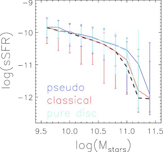
sSFR of the matched bulge samples and pure disc sample (solid lines are median value, and error bars give 68 per cent distribution) as a function of galaxy stellar mass. Blue, red, and cyan lines are for pseudo-bulge, classical bulge, and pure disc samples, respectively. Median result of one corresponding control samples is shown by black dashed line.
We have further examined the possible contribution of the Nneighbour-sSFR connection to our results by additionally matching the pseudo-bulge samples with the control samples in sSFR. The neighbour counts and the ratios to the control samples are shown in Fig. 7. Although the overall amplitudes of the Nneighbour ratio become more noisy, the general trends and our conclusions remain unchanged. Apparently the small-scale enhancement in the neighbour counts as found in our samples and the similar enhancement as previously found by Li et al. (2008a) in strongly star-forming galaxies are not the same effect.

3.3 Close neighbour enhancement in pseudo-bulge and pure disc samples
In the stellar mass range of |$10^{10-11}\, \mathrm{M}_\odot$|, pseudo-bulge and pure disc galaxies show similar excess of neighbour counts with respect to the control samples. At lowest and highest mass bins, the error bars become relatively large, due to the small sizes of the matched galaxy samples when all the samples of pseudo-bulge, classical bulge, and pure disc in a given stellar mass bin are required to be closely matched in various properties. In order to see the difference between pseudo-bulge and pure disc galaxy samples with better statistics, we have repeated the analysis in Fig. 5, but matching only pseudo-bulge and pure disc samples to have similar colour, concentration, and redshift. The results in the stellar mass range of |$10^{9-11}\, \mathrm{M}_\odot$| are shown in Fig. 8. The errors of the neighbour counts and their ratios to the control samples are reduced as expected, particularly for pure disc galaxy samples, and qualitatively the results remain the same as what we see from Fig. 5 – the neighbour count amplitudes at scales smaller than |${\sim }0.1 \, h^{-1}$| Mpc are significantly enhanced when compared to control galaxies of similar mass, for both pseudo-bulges and pure disc galaxies and at all stellar masses.
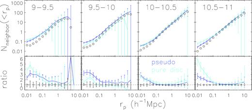
Similar as Fig. 5, but for pseudo-bulge and pure disc galaxies matched with the same distributions of redshift, colour, and concentration, while control samples are also constructed to have the same distributions. Stellar mass bins are in the range of |$10^{9-11}\, \mathrm{M}_{\odot }$|.
Fig. 8 shows that, quantitatively, the Nneighbour ratio of the pseudo-bulges presents a clear anticorrelation with stellar mass, with the small-scale Nneighbour ratio decreasing from ∼3 at the lowest masses to ∼2 at the highest masses. For pure disc galaxies, the Nneighbour ratio at the small scales depends on stellar mass in a non-monotonic manner – the small-scale enhancement in the neighbour count is lowest at |$M_{\mathrm{ stars}}=10^{9.5-10}\, \mathrm{M}_\odot$|, and increases at both higher and lower masses.
The non-monotonic mass dependence of pure disc galaxies can be seen more clearly in Fig. 9 (see the right-hand panel), where we show the pure disc galaxy-to-control ratio as a function of rp for all the stellar mass bins in a single panel. The Nneighbour ratios are consistent at unity within errors on scales larger than |${\sim } 0.1 \, h^{-1}$| Mpc, and increases significantly at smaller scales, reaching a value of 5 or 6 at the smallest scales in both the lowest mass bin (|$10^9\lt M_{\mathrm{ stars}}\lt 10^{9.5}\, \mathrm{M}_\odot$|) and the highest mass bin (|$10^{10.5}\lt M_{\mathrm{ stars}}\lt 10^{11}\, \mathrm{M}_\odot$|). At the intermediate masses, the ratio is at levels of 2–3. In the left-hand panel of the same figure, the results are plotted in the same way for the samples of pseudo-bulge galaxies. The Nneighbour ratios also go beyond unity at small scales with |$r_p\lt 0.1 \, h^{-1}$| Mpc, but they are highest at the lowest masses and decrease with increasing mass monotonically at fixed scale.
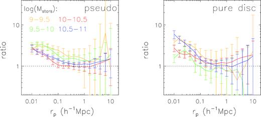
The ratio between neighbour counts of the matched pseudo-bulge (left-hand panel) and pure disc (right-hand panel) galaxy samples and that of the corresponding control sample, for four stellar mass bins indicated by different colour. Error bars show bootstrap errors of the matched galaxy samples.
The neighbour counts we have obtained so far are based on the photometric sample down to a r-band limiting magnitude of rlim = 20. In Fig. 10, we examine the dependence of neighbour counts on rlim, showing the Nneighbour ratios between the matched galaxy samples and the control samples for three different magnitude limits: rlim = 20, 19, and 18. Pseudo-bulge and pure disc samples are the same as shown in Figs 8 and 9. Each panel compares the results of the three limiting magnitudes but for a given stellar mass bin, and results for the pseudo-bulge samples and those for the pure disc galaxy samples are shown in upper and lower panels, respectively. In general, for a given stellar mass bin, the Nneighbour ratio depends very weakly on rlim. This indicates that the excess of the neighbour counts on small scales is dominated by relatively bright companions with r < 18, while fainter neighbours contribute little.
The ratio between neighbour count of matched pseudo-bulge (upper panels) and pure disc (bottom panels) galaxy samples and that of the corresponding control sample, for four stellar mass bins. Solid, dotted, and dashed lines correspond to the results of r-band limiting magnitude of rlim = 20, 19, and 18, respectively. Error bars on the dotted lines show bootstrap errors for results of rlim = 19.
4 DISCUSSION
4.1 Bulge and large-scale environment
On scales larger than a few |$\times 100 \, h^{-1}$| kpc we see no difference in both the two-point cross-correlations and the neighbour counts for all of our samples, when they are matched to have similar mass, colour, and concentration parameter. This implies that the presence of a central bulge and the bulge type in a galaxy are not affected by environmental effects occurring at intermediate-to-large scales. This result is well consistent with previous studies of galaxy clustering and environment. For instance, Li et al. (2006a) estimated the two-point autocorrelation function of SDSS galaxies as a function of their stellar mass, optical colour, and galaxy structure for spatial scales above |$0.1 \, h^{-1}$| Mpc, and found the clustering amplitude at given scale shows obvious dependence on colour but no dependence on concentration and surface mass density when stellar mass is limited to a narrow range. Studies of the local environment of SDSS galaxies have led to the same conclusion: the environment of a galaxy does not relate to its overall structure once the stellar population age and stellar mass are fixed (see a review by Blanton & Moustakas 2009, and reference therein).
For pure-disc galaxies without an obvious bulge component, some of the recent studies have suggested that this class of galaxies are preferentially found in low-density regions (e.g. Kautsch, Gallagher & Grebel 2009), and that a subset of them with a very thin disc tend to avoid filamentary structure on large scales (Bizyaev et al. 2017). We have examined the latter effect using our galaxy samples and the large-scale structure (LSS) type provided by Wang et al. (2016). These authors obtained the initial density field for the local Universe based on the distribution of galaxy groups in the SDSS volume, and reconstructed the three-dimensional density field of the local Universe, as well as its formation history, by running a high-resolution N-body constrained simulation. The density field reconstruction provides not only the local density averaged over 1–3 Mpc scale for each real galaxy in the SDSS volume, but also the type of the LSS in which the galaxy resides. The LSSs in the density field are classified into four different types: void, sheet, filament, and halo, determined from the density field in a dynamical way following Hahn et al. (2007). The density field is limited to local galaxies with redshifts less than |$z$| ∼ 0.12, and includes more than 70 per cent of our galaxies.
Fig. 11 displays the fraction of the galaxies in our sample associated with sheet, filament, or halo, as a function of stellar mass. Results for galaxy samples of classic bulge, pseudo-bulge, and pure disc are plotted with different colours. We don’t consider the LSS type of void in this analysis because of too small a fraction of galaxies falling in this class (less than 4 per cent in all samples). In general, we see very similar fractions at given stellar mass and LSS type. The majority of the galaxies are found in filaments, with a fraction of |${\sim }60{{\ \rm per\ cent}}$| that is little dependent on stellar mass. About 20 per cent of the galaxies in the lowest mass bin are found in sheets, and the fraction decreases at higher masses, reaching zero at the highest masses. The rest |${\sim }20{{\ \rm per\ cent}}$| of the lowest mass bin are found in haloes, but the fraction increases with increasing mass, reaching about 50 per cent at the highest masses. These trends are all well expected, and the similarity between the samples of different morphologies and the control samples suggests again that the presence and type of galactic bulges have little to do with large-scale environments. We note that the pure disc galaxy sample seems to have a slightly higher fraction of the sheet type and correspondingly lower fraction of the halo type, while the bulge samples tend to show a slightly lower fraction of sheet but higher fraction of halo types. However, given the error bars, these subtle differences should not be overemphasized here, and more work with larger samples is needed in order to better understand these differences. With the current data, we find no obvious evidence for any type of our galaxies to either prefer or avoid the filament structure.
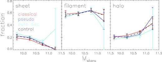
Fraction of galaxies in different large-scale structures (left-hand panel: sheet; middle panel: filament; right-hand panel: halo) as a function of galaxy stellar mass, for galaxy samples and control samples matched with the same distributions of redshift, colour, and concentration in each stellar mass bin. The error bars of the bulge samples are Poisson errors, where for the control samples, dashed lines with error bars give the median value, and the variation range of the 20 control samples constructed for given stellar mass bin.
4.2 Bulge and small-scale environment
Different from what we’ve seen on large scales, on scales less than ∼0.1 Mpc, we have observed significant excess in the close neighbour counts around our galaxies when compared to control galaxies of similar mass, colour, and concentration. The strength of the excess depends on both morphology/bulge type and stellar mass. For classical bulges, the small-scale excess is obviously seen only at low mass (|$M_{\mathrm{ stars}}=10^{9.5-10}\, \mathrm{M}_\odot$|), where the ratio between the classical bulge sample and the control sample reaches ∼5 at the smallest scales (|$r_\mathrm{ p}\sim 10 \, h^{-1}$| kpc, see Fig. 5). If we believed that classical bulges form by major mergers as mentioned in Section 1, our result may be suggesting that classical bulges in massive galaxies with |$M_{\mathrm{ stars}}\gt 10^{10}\, \mathrm{M}_\odot$| are post-merger remnants, thus showing no excess in close neighbour count compared to control galaxies, and that less massive galaxies with |$M_{\mathrm{ stars}}\lt 10^{10}\, \mathrm{M}_\odot$| might still be forming bulges. However, we note that our sample of classical bulges in the lowest mass bin is quite small, resulting in large errors in the neighbour counting as can be seen form Fig. 5. The highly excess of close neighbour counts around classical bulges in low-mass galaxies as reported here need to be double checked in next works with larger samples. If it is proved by future larger samples, our result means that low-mass classical bulges, unlike the more massive ones, prefer to live in relative denser local regions and may form from a different mechanism, such as interaction-induced clumpy disc instability that happens more often and form classical bulges at high redshifts.
The most striking result of our work is that both pseudo-bulge galaxies and pure-disc galaxies show significant enhancement in close neighbour counts when compared to control galaxies of similar mass, colour, and concentration. The result holds even when the distribution of specific star formation rate is additionally matched when constructing the control sample. In some cases, the close neighbour count enhancement is even stronger than the enhancement in the same quantity previously measured for the most strongly star-forming galaxies in SDSS (Li et al. 2008a,b). Furthermore, we found that the neighbour count enhancement doesn’t change much when we include fainter and fainter neighbour galaxies in the counting, which is done by increasing the limiting magnitude of the photometric reference sample. This indicates that the neighbour count enhancement is dominantly contributed by relatively bright neighbours. Our result implies strong connections between pseudo-bulges, pure-disc galaxies, and galaxy–galaxy interactions, although it is not quite clear how they are physically linked with each other.
While we are focusing on the statistics of relative large galaxy samples of different bulge types, some works analyse the properties of galaxies hosting classical and pseudo-bulges based on more detailed identification of smaller samples of galaxies (Fernández Lorenzo et al. 2014), especially for S0 and spiral galaxies (Mishra et al. 2017b; Mishra, Wadadekar & Barway 2018). Mishra et al. (2017a) showed that the existence of different bulge types depends on environment, consistent with our findings that pseudo-bulge and classical bulge have different neighbour counts. Mishra et al. (2017a) and Barway et al. (2017) showed that the formation of pseudo-bulges seems to be independent of environment, possibly on the same line of our results that pseudo-bulges and pure discs have similar excess of close neighbour counts and hence similar small-scale environment.
Recent studies of bulge formation/growth have been mostly focusing on high-z galaxies, where galaxy–galaxy interactions appear to play less important roles than previously expected. For instance, Tadaki et al. (2017) found a large fraction of the extended rotating discs at |$z$| ∼ 2 to be associated with extremely compact centre, dusty, and strongly star forming, which can rapidly build-up a central bulge in a few ×108 yr. Therefore, the authors suggested that bulges are commonly formed in high-z discs by internal processes, not requiring major mergers. However, the situation is quite different when one goes to lower redshifts. In another recent study, Sachdeva, Saha & Singh (2017) studied bulges in bright disc galaxies at |$z$| ≲ 1 using data from both the GOODS-South (0.4 < |$z$| < 1) and SDSS (0.02 < |$z$| < 0.05) samples, concluding that clump migration and secular processes alone cannot account for the bulge growth since |$z$| ∼ 1, and that accretion and minor mergers would be required to explain their data. Our result is apparently along the same line with their work.
5 CONCLUSION
In this work, we have investigated the clustering and close neighbour counts for galaxies with different types of galactic bulges and stellar masses. For this purpose, we have selected samples of galaxies with ‘classic’ or ‘pseudo’ bulges, as well as samples of ‘bulge-less’ pure disc galaxies, using the photometric catalogue of Simard et al. (2011) who performed a careful bulge-disc decomposition on the optical image of a large sample of galaxies in the SDSS. For a given galaxy sample, we have estimated the projected two-point cross-correlation function |$w$|p(rp) with respect to a reference sample consisting of about half a million spectroscopically observed galaxies, and the average background-subtracted neighbour count within a projected separation Nneighbour(<rp) using a photometric reference sample down to r-band limiting magnitude of rlim = 20. In order to isolate out the known correlations between the local environment and galaxy properties such as stellar mass, colour, and structural parameters, we have divided the galaxies into narrow ranges of stellar mass and closely matched the samples in a given mass range, so that the samples of different morphologies and bulge types have similar distributions in redshift, g − r and concentration parameter R90/R50.
Our main conclusions can be summarized as follows:
When limited to a certain stellar mass range and closely matched in redshift, colour, and concentration, all the samples are found to present similar clustering amplitudes and average neighbour counts on scales larger than |${\sim }0.1 \, h^{-1}$| Mpc. This indicates that neither the presence of a galactic bulge nor the type of the bulge is linked to intermediate-to-large scale environments.
On scales less than |${\sim } 0.1\, h^{-1}$| Mpc, the galaxies with a classic bulge present similar clustering properties and neighbour counts to control galaxies of similar mass, colour, and concentration, and this is true for all the scales probed and at all the masses except the lowest mass bin of |$10^{9.5}\lt M_{\mathrm{ stars}}\lt 10^{10}\, \mathrm{M}_\odot$|. In the lowest mass bin, galaxies of classic bulges appear to have more neighbours than the control galaxies, indicating that the presence of a classic bulge in low-mass galaxies is linked to galaxy-galaxy interactions or mergers.
Galaxies with a pseudo-bulge have more close neighbours within |${\sim }0.1 \, h^{-1}$| Mpc when compared to control galaxies of similar mass, colour, and concentration, with the average neighbour count being enhanced by a factor of 2–3 at the smallest scales. The enhancement is weakly anticorrelated with stellar mass, with the sample-to-control Nneighbour ratio slightly decreasing with increasing mass.
Pure disc galaxies with no bulges also show enhanced close neighbour counts within |${\sim }0.1 \, h^{-1}\mathrm{ Mpc}$| compared to the control galaxies, but the enhancement depends on stellar mass in a non-monotonic way, with the highest sample-to-control Nneighbour ratio occurring at both high and low masses. As a consequence, galaxies at intermediate masses (|$M_{\mathrm{ stars}}\sim 10^{9.5-10}\, \mathrm{M}_\odot$|) present the weakest signal. The Nneighbour ratio increases to the levels of 5–6 at |$M_{\mathrm{ stars}}\gt 10^{10.5}\, \mathrm{M}_\odot$| and |$M_{\mathrm{ stars}}\lt 10^{9.5}\, \mathrm{M}_\odot$|, an effect which is similar or even stronger than the previous measurement of the same quantify for the most strongly star-forming galaxies in the SDSS.
Note that in this work, we select only a very small fraction of galaxies with robust bulge type determinations based on the SDSS dr7 catalogue. Due to the limited numbers of galaxies selected, our matched samples are dominated by blue and low-concentration galaxies (Fig. 3). With future high spatial resolution observational data, and more accurate bulge-to-disc decomposition measurement that takes into account the components of nuclear and inner lenses/rings (Gao & Ho 2017), the clustering properties and other statistics of galactic bulges could be better derived, to set more constraints on the formation of galactic bulges. In addition, theoretical studies are also needed in order to have a full understanding of the formation process of bulges of both classical and pseudo-types, as well as the physical relationship with pure-disc bulgeless galaxies. According to our study, these theoretical models must involve galaxy–galaxy interactions and other environment effects over a large range of spatial scales, as well as secular processes internal to galaxies.
ACKNOWLEDGEMENTS
We thank the reviewer for the detailed and helpful comments. We thank Cheng Du, Shude Mao, Liang Gao, and colleagues of the YIPA galaxy discussion group at NAOC for helpful discussions. LW acknowledges support from the National Natural Science Foundation of China grants program (No. 11573031), and the National Key Program for Science and Technology Research and Development (2017YFB0203300). CL is supported by National Key Basic Research Program of China (No. 2015CB857004) and the National Natural Science Foundation of China (grant No. 11173045, 11233005, 11325314, 11320101002). CL, HJM, and HYW are also supported by the National Key Basic Research and Development Program of China (No. 2018YFA0404502, No. 2018YFA0404503).
Funding for the SDSS and SDSS-II has been provided by the Alfred P. Sloan Foundation, the Participating Institutions, the National Science Foundation, the U.S. Department of Energy, the National Aeronautics and Space Administration, the Japanese Monbukagakusho, the Max Planck Society, and the Higher Education Funding Council for England. The SDSS Web Site is http://www.sdss.org/. The SDSS is managed by the Astrophysical Research Consortium for the Participating Institutions. The Participating Institutions are the American Museum of Natural History, Astrophysical Institute Potsdam, University of Basel, University of Cambridge, Case Western Reserve University, University of Chicago, Drexel University, Fermilab, the Institute for Advanced Study, the Japan Participation Group, Johns Hopkins University, the Joint Institute for Nuclear Astrophysics, the Kavli Institute for Particle Astrophysics and Cosmology, the Korean Scientist Group, the Chinese Academy of Sciences (LAMOST), Los Alamos National Laboratory, the Max-Planck-Institute for Astronomy (MPIA), the Max-Planck-Institute for Astrophysics (MPA), New Mexico State University, Ohio State University, University of Pittsburgh, University of Portsmouth, Princeton University, the United States Naval Observatory, and the University of Washington.
Footnotes
The catalogue is publicly available at: http://www.sdss.org/dr12/spectro/galaxy_mpajhu/.
NYU-VAGC catalogue can be found at: http://sdss.physics.nyu.edu/vagc/.
REFERENCES
APPENDIX A: UNCERTAINTY IN THE FITTING OF SERSIC PARAMETER
In Simard et al. (2011), when fitting galaxies with a free nb bulge + disc model, and a pure Sersic ng model, the Sersic index n is set to be within the range of 0.5 < n < 8. In Fig. A1, we plot the distribution of error in n in our samples, before excluding galaxies with n ≥ 7.95. Classical B sample galaxies have nb = 4 with no error and are therefore not presented in the figure. Solid lines are the median value at given n, and dashed lines include 68 percentile distribution around the median. We have checked that when excluding galaxies with error in nb greater than the +1σ of error distribution (above the upper dashed lines) in our samples, and do the same matching of samples to make them have the same distribution of redshift, colour, and concentration, the resulting correlation function and neighbour count results remain similar. This means that these galaxies with large error in n fitting do not affect our conclusion qualitatively.
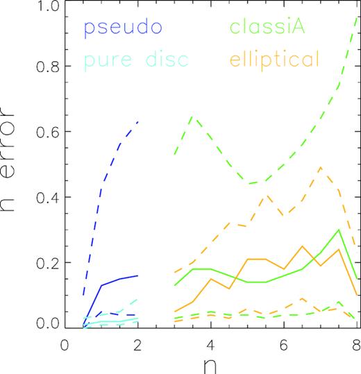
The error of n in our samples. Solid lines are the median error of n at given n value, while dashed lines include 68 per cent distribution of n error around the median.
When galaxies host bars, the fitting bulge Sersic indices may be affected since the models adopted by Simard et al. (2011) do not include the bar components. If the existence of bars significantly affect the fitting of Sersic indices, it should increase the resulting n values and hence the fraction of classical bulge galaxies with bars should be larger than that of the pseudo-bulge sample. To check the effect of bars on the determination of Sersic indices, we have cross-matched our samples with the morphological catalogue provided by Nair & Abraham (2010), which includes detailed visual classifications for 14 034 galaxies in SDSS. The matched number of galaxies in the pseudo-bulge sample is 727, among which 26.5 per cent host bars. The matched number of galaxies in the classical bulge sample is 2702, and 21.9 per cent host bars. The percentage of barred system is a bit higher in the pseudo-bulge sample. Therefore the existence of bars is not significantly increasing the n values of the samples. Also note that the clustering as well as the neighbour counts of barred and unbarred galaxies of similar stellar mass is indistinguishable (Li et al. 2009; Lin et al. 2014), although bar growth and classical bulges may be related (Barway et al. 2016). Therefore the existence of bars would not affect of the results of our selected galaxy samples.
APPENDIX B: KORMENDY DIAGRAM AND VELOCITY DISPERSION OF OUR SAMPLE GALAXIES
Kormendy (2016) provides the latest complete list of bulge classification criteria, which includes sSFR, velocity dispersion, bulge-to-total ratio, Sersic index, etc. Any one criterion has a non-zero probability of failure in determining the type of galactic bulges. Therefore the use of more classification criteria can give more reliable results. For example, Vaghmare et al. (2015) combined the n < 2 criterion with the offset in the Kormendy diagram (Kormendy 1977) to select pseudo-bulges. Mishra et al. (2017b) added one more criterion to select pseudo-bulges to have velocity dispersion less than |$130 \, \mathrm{km\, s}^{-1}$| (Fisher & Drory 2016).
We should note, however, while the significant offset in the Kormendy diagram is useful to define typical pseudo-bulges, identifying classical bulges using this relation is not robust (Fisher & Drory 2016), since some pseudo-bulges also fit the Kormendy relation (Kormendy 2016). Besides, Kormendy relation cannot be used to separate pseudo-bulges from classical bulges in dwarf galaxies, since both types of bulge depart from this relation at low-luminosities (Graham 2016). On the other hand, including more criteria means including less number of galaxies in the selected samples, and would make the resulting galaxy samples without enough numbers to do statistics such as correlation functions and neighbour counts. Therefore, in this work, to select pseudo-bulge and classical bulge galaxies, we use the Sersic index to define different bulge types. This is based on the fact that most pseudo-bulges have Sersic index n < 2, while most classical bulges have n ≥ 2 (Kormendy & Kennicutt 2004; Fisher & Drory 2008; Kormendy 2016)
Nevertheless, to check whether using the Sersic index alone causes significant sample contamination and may be biasing our results, we analyse the Kormendy diagram of our selected samples. In Fig. B1, we plot the r-band surface brightness–effective radius relation for our selected elliptical sample. Black solid line is the best-fitting relation for our elliptical sample, while black dotted and dashed lines indicate 1 and 3 rms scatters, respectively. The result is in general consistent with the work of Mishra et al. (2017b), but with a bit larger scatter.
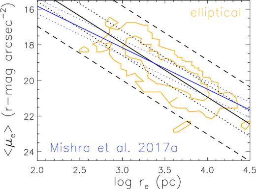
r-band Kormendy diagram of our selected elliptical sample, as presented in Section 2 and Table 1. Two contours include 68 and 95 percentile of galaxies in the sample. Black solid line is the best-fitting relation for our elliptical sample, while black dotted and dashed lines indicate 1 and 3 rms scatters, respectively. As reference, blue solid line shows the best-fitting line for ellipticals using r-band data as presented by Mishra et al. (2017b), with blue dotted lines showing the range of their rms scatter.
In Fig. B2, we plot the position of galaxies on the Kormendy plane for our bulge samples. Most of the classical galaxies lie within the scatter of the Kormendy relation defined by our elliptical sample (dashed lines), with some exceptions lying below the relation. Pseudo-bulges have a much larger fraction lying below the lower dashed line. In both Vaghmare et al. (2015) and Mishra et al. (2017b), pseudo-bugles are required to lie below three times the rms of the best-fitting line to the elliptical sample. Following their criterion, we select further our bulge samples according the Kormendy relation. Pseudo-bulge galaxies with Kormendy criterion (pseudo-Kor) are required to be below the lower dashed line in Fig. B2, and contain 30.0 per cent galaxies in our original pseudo-bulge sample. Classical bulge galaxies with Kormendy criterion (classical-Kor) are required to be above the lower dashed line in Fig. B2, and contain 90.0 per cent galaxies in our original classical bulge sample.
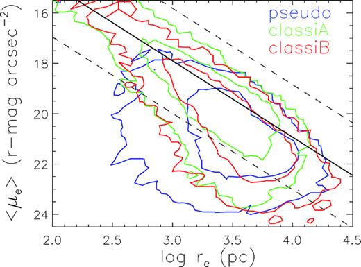
r-band Kormendy diagram of our selected sample of pseudo-bulge, classical bulge A, and classical bulge B, as presented in Section 2 and Table 1. For each sample, two contours include 68 and 95 percentile of galaxies in the sample. Black solid line is the best-fitting line for our elliptical sample, and dashed lines show the range of three times the rms scatter, which are the same as shown in Fig. B1.
With the additional constraint based on the Kormendy diagram, we check the neighbour counts results of the pseudo-Kor and classical-Kor samples. To make a fair comparison, the galaxies in both the pseudo-Kor and classical-kor are matched with the samples shown in Fig. 5 to have the same distributions in redshift, colour, and concentration in each stellar mass bin. The resulting numbers of galaxies in the two-Kor samples are small, which can give enough statistics only in the stellar mass bin of |$10^{10-10.5}\, \mathrm{M}_{\odot }$|, and the result is shown in Fig. B3. Although the bootstrap errors of the two bulge samples are large, compared with the results in the panel of the same stellar mass in Fig. 5, the general conclusion seems to still hold. Pseudo-bulge galaxies have excess in neighbour counts on the small scales, while classical bulges have no excess on small scales.
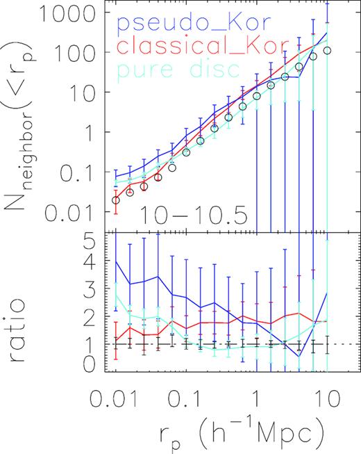
Similar as Fig. 5, but for classical bulge and pseudo-bulge samples with additional constraint based on the Kormendy diagram (see text for the details). In each stellar mass bin, the samples are matched to have the same z, colour, and concentration distributions as the bulge samples and control samples shown in Fig. 5. Due the limited numbers in the matched samples, only results at one stellar mass bin of |$10^{10-10.5}\, \mathrm{M}_{\odot }$| are shown here.
To check the velocity dispersion of our sample galaxies, we have again matched our samples with the catalogue provided by Nair & Abraham (2010), which provide the kinematic information. In Fig. B4, we plot again the Kormendy diagram for our original pseudo-bulge sample. The galaxies with velocity dispersion information (683 in number) are overplotted, while solid dots represent galaxies with velocity dispersion less than |$130 \, \mathrm{km\, s}^{-1}$| (549 galaxies), and open circles are galaxies with larger velocity dispersion (134 galaxies). 227 galaxies with velocity dispersion information are below the lower dashed line, i.e. fulfilling the criterion based on the Kormendy relation, among which 97.4 per cent have velocity dispersion less than |$130 \, \mathrm{km\, s}^{-1}$|. This test indicates that most of the pseudo-bulge galaxies selected based on n < 2 and have large offset on the Kormendy plane also match the velocity dispersion criterion. Nevertheless, as have discussed in the beginning of this section, these criteria are useful to select un-contaminated typical pseudo-bulges, but do not include all pseudo-bulges.
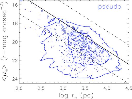
r-band Kormendy diagram of our selected sample of pseudo-bulge, same as in Fig. B2. Overplotted by dots and circles are pseudo-bulge galaxies that have velocity dispersion information matched in the catalogue of Nair & Abraham (2010). Filled dots are galaxies with velocity dispersion less than |$130\, \mathrm{km\, s}^{-1}$|, while open circles are those with larger velocity dispersion.
