


ABSTRACT
We report interferometric observations tuned to the redshifted neutral hydrogen (H i ) 21cm emission line in three strongly lensed galaxies at z ∼ 0.4 with the Giant Metrewave Radio Telescope. One galaxy spectrum (J1106+5228 at z = 0.407) shows evidence of a marginal detection with an integrated signal-to-noise ratio of 3.8, which, if confirmed by follow-up observations, would represent the first strongly lensed and most distant individual galaxy detected in H i emission. Two steps are performed to transcribe the lensed integrated flux measurements into H i mass measurements for all three target galaxies. First, we calculate the H i magnification factor μ by applying general relativistic ray tracing to a physical model of the source-lens system. The H i magnification generally differs from the optical magnification and depends largely on the intrinsic H i mass MH i due to the H i mass–size relation. Secondly, we employ a Bayesian formalism to convert the integrated flux, amplified by the MHI-dependent magnification factor μ, into a probability density for MH i, accounting for the asymmetric uncertainty due to the declining H i mass function (Eddington bias). In this way, we determine a value of |$\log _{\rm 10} (M_{\rm H\,{\small I}}/M_\odot) = 10.2^{+0.3}_{-0.7}$| for J1106+5228, consistent with the estimate of 9.4 ± 0.3 from the optical properties of this galaxy. The H i mass of the other two sources are consistent with zero within a 95 per cent confidence interval however we still provide upper limits for both sources and a 1σ lower limit for J1250−0135 using the same formalism.
1 INTRODUCTION
Neutral atomic hydrogen (H i ) plays a key role in the baryon cycle of galaxies. Its spatial distribution within galaxies is diffuse and extended, with significant mass beyond the stellar component of the galaxy (Leroy et al. 2008). As the simplest, most abundant, and spatially extended galactic gas component, studies of neutral hydrogen can probe a wide range of astrophysics including star formation histories, galaxy interactions, and cosmic large-scale structure. For example, the ratio of the cosmic densities of molecular to neutral hydrogen |${\rm \Omega _{H_2}/\Omega _{\rm H\,{\small I}}}$| is predicted to increase as a function of redshift, for instance as |${\rm \Omega _{H_2}/\Omega _{\rm H\,{\small I}}} \propto (1+z)^{1.6}$| between 0 ≤ z ≤ 2 (Obreschkow et al. 2009). This results from the growth of haloes with cosmic time which leads to larger but less dense galactic discs. The decreasing density of galactic discs at lower redshift are then less efficient at converting H i → H2 due to the reduction in gas pressure. This decline in |${\rm \Omega _{H_2}/\Omega _{\rm H\,{\small I}}}$| with cosmic time parallels the rapid decrease in the co-moving star formation rate (SFR) density from z ∼ 2 to the current epoch (Hopkins & Beacom 2006, and references therein).
Neutral hydrogen can be observed via the 21 cm radio line, which results from the forbidden hyperfine (spin-flip) transition (we refer to this as the H i line). Unfortunately, as the H i emission line is extremely faint, it is difficult to constrain |${\rm \Omega _{\rm H\,{\small I}}}$| at z > 0.2 with direct observations. Currently, the COSMOS H i Large Extra-galactic Survey carried out on the Karl G. Jansky Very Large Array (VLA) holds the record for the most distant detection of H i in emission from a single galaxy with MH i = 2.9 × 10¹⁰ M⊙ at z = 0.37 (Fernández et al. 2016). The detection was reported using the first 178 h of data of the 1002 h survey of the COSMOS field. The redshift cut-off for the survey is at z ∼ 0.45, governed by receiver sensitivity drop at the lower end of the VLA L band, where L band refers to the frequency band ∼1−2 GHz. With the 305 m Arecibo dish, the HIghz project (Catinella & Cortese 2015) detected 39 galaxies |$2 \le M_{\rm H\,{\small I}}/10^{10}\, {\rm M_\odot } \le 8$| at 0.17 ≤ z ≤ 0.25. These H i masses fall at the high end of the H i mass function (HIMF) in the local Universe, well above the point at which the HIMF transitions into an exponential decline (Jones et al. 2018).
Absorption studies of the 21cm line (e.g. Gupta et al. 2013; Allison et al. 2015) and Lyman α (e.g. Prochaska et al. 2011), as well as statistical analyses such as stacking (Verheijen et al. 2007; Kanekar, Sethi & Dwarakanath 2016) and intensity mapping (Chang et al. 2010; Masui et al. 2013), provide important constraints on high-redshift H i , but are strongly model-dependent techniques. Hence, direct detections are critical to cross-check and more directly constrain the high-redshift H i mass function. Future radio telescopes like the Square Kilometre Array (SKA) and its pathfinders/precursors should be able to make detections of individual, massive galaxies towards z ∼ 1. A promising route to higher redshift H i detections with current and future telescopes is the natural flux magnification enabled by strong gravitational lensing.
Amplification of emission through gravitational lensing has been used at many wavelengths to boost the signal of distant, faint galaxies, however there has been no strongly lensed H i detection in emission to date, with only a single published attempt known to the authors (Hunt, Pisano & Edel 2016). Predictions show that targeted observing campaigns should be able to detect lensed H i within reasonable observing times of order a few days with current instruments (Deane, Obreschkow & Heywood 2015). This would allow us to probe lower H i mass galaxies at intermediate redshift, yielding complementary results to large-scale H i surveys in progress/preparation.
In this paper, we present: (1) the results of Giant Metrewave Radio Telescope (GMRT) L-band observations of three galaxy–galaxy gravitational lenses, (2) Monte Carlo simulations of the ray-traced parameteric H i discs to estimate the average (i.e. total H i intensity) magnification, and (3) a Bayesian formalism for a robust description of the H i mass probability. In Section 2, we present the target selection, the observational details and data reduction; in Section 3 we present the interferometric data products (Section 3.1), the H i lensing simulations (Section 3.2) and the H i mass probability distributions (Section 3.3). In Section 4, we present the key results of the H i mass constraints and the magnification estimates and apply these to speculate on the impact of lensing on future observations. Section 5 summarizes the paper and presents our plan for future work in the field. We assume a Planck 2015 cosmology (Planck Collaboration XIII 2016) throughout. See Table 1 for summary of observation details, the source parameters, and our final results.
Summary of source properties and derived results for three strongly lensed sources. The first section of the table is largely taken from Newton et al. (2011) and is based on SDSS spectroscopy and HST imaging, although see Section 2.3 for discussion of the source redshifts. The H i mass predictions are interpolated from Maddox et al. (2015) as described in the text. The impact factor ranges used in the simulations are estimated in Section 3.2.2. The second section describes the basic observational setup at the GMRT, and the third section presents the observational results. The fourth section details the derived H i mass and magnification and constraints (see Fig. 5 for a visual representation). The final line presents an H i mass upper limit using the alternative method discussed in Section 4.1.
| J1106+5228 | J1250−0135 | J1143−0144 | |
|---|---|---|---|
| Co-ordinates | 11h06m46|${^{\rm s}_{.}}$|15+52d28m37|${^{\rm s}_{.}}$|8 | 12h50m50|${^{\rm s}_{.}}$|52−01d35m31|${^{\rm s}_{.}}$|7 | 11h43m29|${^{\rm s}_{.}}$|64−01d44m30|${^{\rm s}_{.}}$|0 |
| zlens | 0.095 | 0.087 | 0.106 |
| zsrc (optical) | 0.4070 ± 0.0003 | 0.3526 ± 0.0004 | 0.4019 ± 0.0004 |
| zsrc (H i ) | 0.4073 | 0.3526 | 0.4019 |
| μ (optical) | 28 | 13.3 | 10.4 |
| log10M⋆/M⊙ | |$8.72^{+0.23}_{-0.12}$| | |$9.37^{+0.14}_{-0.15}$| | |$9.00^{+0.23}_{-0.15}$| |
| Einstein radius (arcsec) | 1.23 ± 0.14 | 1.28 ± 0.12 | 1.68 ± 0.14 |
| Intrinsic optical isophotal radius (arcsec) | 0.11 | 0.25 | 0.15 |
| Predicted log10MH i/M⊙ | 9.4 ± 0.3 | 9.7 ± 0.3 | 9.5 ± 0.3 |
| Impact factor range (arcsec) | [0, 0.1] | [0, 0.2] | [0.2, 0.4] |
| On-source observing time (h) | 6.8 | 16.5 | 4.5 |
| Bandwidth (MHz) | 4 | 32 | 4 |
| Channel resolution (kHz) | 8 | 64 | 8 |
| Mean no. of working antennas | 26 | 26 | 28 |
| RMS of continuum image (|$\mu$|Jy beam−1) | 54 | 16 | 64 |
| Spectral line uv-weighting | Natural | Briggs 0.5 | Briggs 0.5 |
| Frequency-integrated flux (Jy Hz) | 414 | 114 | −84 |
| RMS of spectral line (Jy Hz) | 110 | 69 | 102 |
| Probability of zero mass (C0) | 10−4 | 0.04 | 0.79 |
| 〈μ〉 at optically predicted mass | 3.9 | 2.3 | 3.3 |
| 〈log10MH i/M⊙〉 | 10.2 | 9.4 | − |
| 〈μ〉(〈log10MH i/M⊙〉) | 1.9 | 3.1 | − |
| 68% conf. bounds on log10MH i/M⊙ | [9.5, 10.5] | [8.1, 10.0] | [–, 8.0] |
| 95% conf. bounds on log10MH i/M⊙ | [7.8, 10.8] | [–, 10.3] | [–, 9.7] |
| 99.7% conf. bounds on log10MH i/M⊙ | [6.4, 10.8] | [–, 10.4] | [–, 10.1] |
| 3σ upper limit (log10MH i/M⊙) | 10.7 | 10.4 | 10.7 |
2 OBSERVATIONS AND REDUCTION
2.1 Targets
All three sources are galaxy–galaxy lenses selected from the Sloan Lens ACS Survey (SLACS) lens catalogue (Bolton et al. 2008; Auger et al. 2009; Newton et al. 2011). We emphasize that we are interested in detecting H i in the lensed galaxy and not the lensing galaxy. These strong lenses were identified via a search through the SDSS spectroscopic data for an absorption-dominated spectrum consistent with an early-type galaxy at one redshift and nebular emission lines (Balmer series, [O ii] and [O iii]) consistent with a star-forming galaxy at a higher redshift. Given the 3 arcsec fibre diameter, such composite spectra would provide strong evidence of two separate galaxies and hence a lens candidate. The resulting candidates were observed with the Hubble Space Telescope (HST) in bands VHST, I814, and H160 to confirm and model the lens. The original SLACS sample consisted of 85 ‘grade-A’ (i.e. showing clear signs of multiple imaging) lensed systems (Auger et al. 2009), 46 of these were further studied by Newton et al. (2011) to extract information about the source characteristics. These sources lie between 0.2 ≤ zsrc ≤ 1.3 with a median modelled (unlensed) stellar mass of log10(M⋆/M⊙) = 8.85 and a median optical magnification of 8.8.
There were several reasons for using the SLACS catalogue for H i candidate selection. First, it is the largest spectroscopic catalogue of low to intermediate redshift (0.2 ≲ zsrc ≲ 1) lensed galaxies available. Secondly, as the targets have strong nebular emission lines, they are star forming and hence may likely have significant cold gas reservoirs. Thirdly, as the lenses had been well modelled in the optical with HST data, these models could then be utilized for H i analysis. All three targets in our observations were categorized as ‘grade A’ lenses in the catalogue.
Fig. 1 shows the estimated H i integrated flux as a function of redshift, using the M⋆−MH i correlation12 presented in Maddox et al. (2015) and the naive assumption that H i magnification is equivalent to the optical magnification. The validity of the assumption on the magnification will be explored later in the paper. The predicted H i masses of our targets (see Table 1) lie in the range log10(MH i/M⊙) = 9.5 ± 0.5.
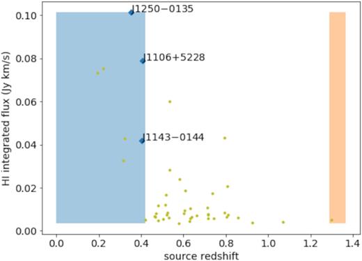
Predicted integrated H i flux as a function of source redshift for SLACS sources described in Newton et al. (2011), using the M⋆−MH i conversion given in Maddox et al. (2015) and the naive assumption that optical magnification is equal to H i magnification. Observed sources reported in this work are indicated by the blue diamonds and text, while the other sources in the catalogue are shown as yellow dots. The GMRT L band is shown in blue (identical to the VLA L band) and the GMRT UHF band is shown in red.
We observed three SLACS sources with the GMRT: J1106+5228, J1250−0135, and J1143−0144, shown in Fig. 1. Our sources were selected out of the SLACS sample by (1) observability from the GMRT near Pune, India and (2) the predicted magnified H i integrated flux. The first section of Table 1 shows a summary of the observational parameters, including source and lens redshifts.
2.2 Data reduction
In order to benefit from new interferometric data reduction software development, we designed a data processing pipeline using the stimela3 interface (Makhathini 2018). This provided a consistent interface over a variety of software tools, e.g. aoflagger (Offringa 2010), wsclean (Offringa et al. 2014), pybdsf (Mohan & Rafferty 2015), casa (McMullin et al. 2007), cubical (Kenyon et al. 2018), and meqtrees (Noordam & Smirnov 2010).
The entire reduction can be roughly divided into three broad sections (known as generations of calibration). In the first, the calibrator fields provide the initial antenna-based complex gain solutions as a function of time and frequency. The frequency-dependent solutions are fixed in at this point. In the second (self-calibration), the target field itself is used to further calibrate the antenna gains, with iterations over decreasing time intervals. Note that the continuum fields contain many bright sources not associated with the target galaxy. It is these objects upon which the self-calibration operates and not the target or lens galaxy which are typically faint. In the third, we try to minimize artefacts caused by direction-dependent gains imparted to bright off-axis sources (Smirnov 2011). These direction-dependent gain errors result from fluctuations in the primary beam pattern due to antenna pointing errors. The time-dependent gain solutions are only fixed in at the endpoint of the calibration.
The typical duty cycle was 3 min on the gain calibrator followed by 15 min on the source, with 15 min scans on the flux (primary) calibrator at the beginning and end of each observation.
The reduction of the calibrator fields made use of the standard casa calibration routines and wsclean for imaging. Both manual and automated flagging was carried out, the latter with aoflagger following several tests to find an optimal aoflagger strategy. We minimize the impact of radio frequency interference (RFI) on calibration solutions by performing two calibration steps on the calibrators. In the first step, we flag and calibrate. In the second step, we subtract the calibrator source model from the visibilities, flag the residuals and solve again for the calibration solutions. The bandpass solutions showed fluctuation across the band, especially for the 32 MHz band due to the decrease in channel resolution.
During self-calibration, we used on the order of five calibration-source modelling loops. For accurate deconvolution and continuum subtraction in the target fields, we experimented with different combinations of wsclean automasking and multiscale settings as well as pybdsf for modelling sources as parametric components. RFI flagging with aoflagger was used for the target fields as well, but with higher flagging thresholds in order to retain as much data as possible. When we solve for the antenna gain solutions during calibration, we first apply the older (longer time interval) solutions. This ensures that the new gains start closer to an optimized solution, especially as the signal-to-noise ratio (SNR) drops for smaller solution intervals. The SNR of the continuum fields were high enough for this step to be successful and in general the self-calibration step increased the image SNR by approximately a factor of 2. After the final calibration step, the model of the continuum sky is subtracted from the data.
We now present a brief discussion on the reduction of each individual field. A summary of each field can be found in Table 1.
2.2.1 J1106+5228 (z = 0.407)
This field is dominated by two ∼0.1 Jy off-axis point sources, on diametrically opposite parts of the field of view. The two sources are 11 and 17 arcmin away from the phase centre. The half-power radius of the GMRT primary beam at this wavelength is ∼14 arcmin. The multiplication (in the image plane) of the time-dependent primary beam pattern with bright, off-axis sources causes errors most prominent in the immediate vicinity of the sources in question. We used a differential gain technique to solve for these sources with meqtrees and cubical, however the limited bandwidth (4 MHz) and source flux meant that the SNR was too low for differential gain solutions to converge.
2.2.2 J1250−0135 (z = 0.353)
This field is dominated by a bright off-axis radio galaxy with complex, extended morphology not readily seen in previous, lower angular resolution maps. This well-resolved source is situated at an angular distance of 12 arcmin from the phase centre (i.e. 85 per cent of the angular distance to the half-power point). We solved for differential gain solutions towards this problematic source, however the SNR was again too low and source structure too complex to see a significant improvement in the image residuals. The significantly poorer uv-coverage for equatorial observations leads to a point spread function (PSF) with significant amplitude outside of the main lobe. The combination of the complex, diffuse source structure, primary beam effects and a PSF with significant side-lobes meant that this source could not be robustly modelled and hence accurately subtracted from the data. For this reason, we chose to extract the spectra of this target with a Briggs 0.5 weighting, suppressing the PSF side-lobes at the expense of a slight sensitivity penalty.
2.2.3 J1143−0144 (z = 0.402)
This is also an equatorial field, which meant that the PSF had high interferometric side-lobes. Due to the presence of large-scale diffuse emission close to the target (likely associated with the parent cluster of the foreground galaxy lens), we choose Briggs 0.5 weighting for the spectral line science with this target, in this case to suppress the shortest spacings and thus the sensitivity to the diffuse foreground emission.
2.3 Spectral line width and centre
The analysis of marginal or non-detections of H i is complicated by potential misalignment of the H i and optical emission line centroids in redshift space. Misalignments can be either due to the measurement uncertainty associated with the spectral lines or intrinsic physical offsets between the emitting components. Intrinsic offsets between the optical and H i redshifts could occur for a variety of reasons including stellar outflows or asymmetries in the stellar or H i discs (Maddox et al. 2013).
There are two additional complications to centroid alignment relevant to this galaxy sample. As the SDSS fibre radius (≈1.5 arcsec) is comparable to the size of the Einstein radii (see Table 1), some of the emission may not be captured. Furthermore, although lensing is achromatic, intrinsic spatial variation between ionized and neutral gas would result in differing magnifications. An example of a differentially magnified spectrum is shown in fig. 1 of Deane et al. (2015).
As the original SLACS papers did not quote an uncertainty on the redshift, we re-derive the redshifts along with uncertainties. To do this, we subtract the SDSS model of the foreground galaxy spectrum, and fit a Gaussian profile to the high SNR ([O iii] 5008 Å) line. To factor in the possibility of a misalignment between the optical and H i centroids as discussed above, we use the width of the profile (∼100 km s−1) instead of the uncertainty on the peak position (∼10 km s−1). The expectations of these re-derived redshifts all agree with the Bolton et al. (2008) redshifts within the either choice of uncertainty.
The full line width, defined as 20 per cent of the peak flux w20, can be predicted from the baryonic Tully–Fisher relation (McGaugh et al. 2000). We estimate the baryonic mass using the predicted stellar and H i masses and the ratio of total gas mass to H i mass of 1.5 [roughly accounting for molecular gas mass for star-forming galaxies at this redshift (Geach et al. 2011)]. For an edge-on disc, this yields approximately w20 ∼ 200 km s−1 for all three sources.
To search for possible detections, the radio spectrum is then convolved with a boxcar of size ∼200 km s−1 (expected size in the rest frame) and we check for significant peaks within a redshift range of 1σ from the optical peak.
We then choose two peak thresholds at SNR > 6.5σ [the same as the class 1 sources in the ALFALFA (Arecibo Legacy Fast ALFA) survey (Haynes et al. 2011; Jones et al. 2018)] and SNR > 3σ, the former representing detections and the latter representing follow-up candidates which show evidence of a marginal detection.4 Only for the source J1106+5228 do we find a significant peak with SNR > 3σ, consistent with the O [iii] 5008 redshift within 1σ, offset from the peak by 65 km s−1 (see Table 1 for optical and H i redshift centroids).
We use the integrated flux (i.e. the averaged flux over the 200 km s−1 bin multiplied by the frequency width of the bin) at the optical redshift expectation or at the highest SNR > 3σ peaks if any. The integrated flux values, even the non-detections, are necessary for our novel analysis formalism derived Section 3.3.
3 RESULTS AND SOURCE MODELLING
3.1 Interferometric data products
3.1.1 Spectra
The radio spectra of the targets are shown in Fig. 2. The binned spectra are overplotted in orange, where the bin size is set to the number of channels extended by a rest-frame velocity width of 200 km s−1 (see Section 2.3 for discussion on the bin width).
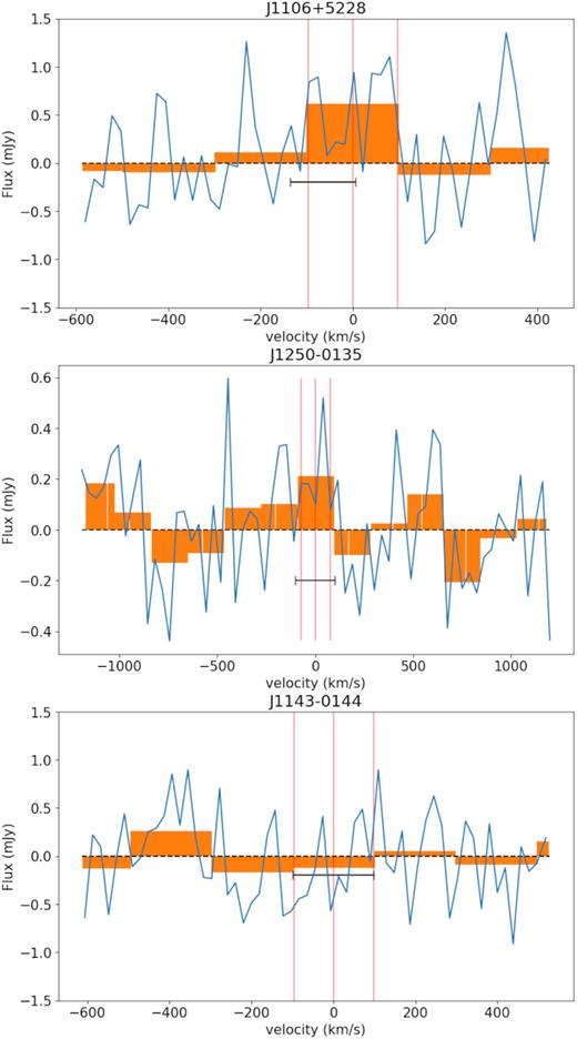
Source position-centred spectra with the rest-frame line position and 200 km s−1 line width indicated by the red vertical lines. The binned spectra are overplotted in orange, where the bin size is set to the number of channels extended by a rest-frame velocity of width of 200 km s−1 at the source redshift. The optical redshift and uncertainty is shown by the horizontal black line. See accompanying text in Sections 3.1.1 and 2.3 for more details. Integrated flux and noise estimates are given in Table 1.
An outer uv-taper (Gaussian, FWHM of 6 arcsec) was used to maximize sensitivity to extended emission. This angular size was predicted by applying the H i mass–size relation to the expected H i mass based on the optical prior. We also subtract the mean of the off-source channels to remove any continuum emission associated with the lens and/or source.
Following from Section 2.3, the rest-frame line position is set to the expectation of the optical redshift for non-detections, except in the case of J1106+5228 where the spectra have been shifted by 65 km s−1 to centre the candidate detection (integrated SNR of 3.8σ) at 0 km s−1. This offset is within 1σ of the optical redshift expectation. The optical redshift and uncertainty is shown by the horizontal black line. At this low SNR, we cannot say with high significance that this detection is real, however the evidence available shows that it would be an excellent candidate for follow-up observations. Because the integrated SNR is only 3.8, it is statistically impossible to determine further parameters (in addition to the integrated flux), such as the line width (200 km s−1) which was set by the optical prior. In contrast to low redshift, high-SNR H i detections, we expect a low-SNR detection, rather than attempting to Nyquist sample the putative lensed H i emission line.
The spectral sensitivity and source-centred (frequency and angular position) integrated fluxes are given in Table 1.
3.1.2 Continuum
The continuum sensitivities are given in Table 1. The continuum image sensitivity scales approximately as |$1/\sqrt{N}$|, where N is the number of unflagged visibilities, and is close to the theoretical noise for continuum images indicating that the calibration, flagging, and source modelling was successful. Approximately 16 per cent of data was flagged in each hand of polarization due to RFI. Unfortunately, the impact of low-level, broad-band undetected RFI is difficult to estimate and separate from other systematic effects like primary beam errors.
We report a continuum detection coincident with the optical position of J1250−0135, shown in Fig. 3. The flux density of this source is 0.53 mJy and we postulate that the emission originates in the foreground (z = 0.087) lens galaxy. The source is unresolved and has a radio luminosity of L1.4GHz ∼ 1023 W Hz−1 which indicates that the radio component is AGN dominated according to the categorization of Mauch & Sadler (2007). The continuum was not detected for the other two sources.
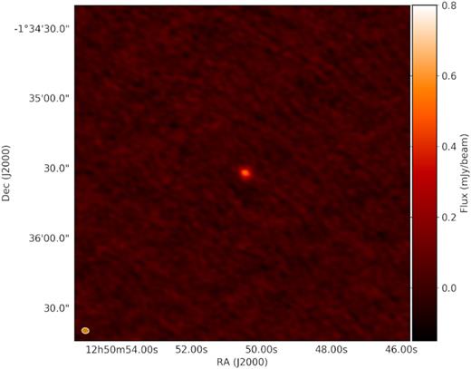
Continuum detection coincident with the published HST-measured position of J1250−0135. The image scale is 2.4 × 2.4 arcmin2. The source has a peak flux of 0.53 mJy, yielding SNR ∼ 30. The synthesized beam is shown in the bottom left corner. The major and minor axes are 3.0 and 2.4 arcsec, respectively.
3.2 H i magnification model
We now seek a quantitative prediction of the H i lensing magnification and hence the expected H i integrated flux for targets. A theoretical estimate of the H i magnification requires: (1) a physically motivated range of possible H i distributions, (2) an accurate model of the lens, and (3) general relativistic ray tracing. We opt for a parametric disc model and explore the dependence of all free parameters on the magnification, marginalizing over the nuisance parameters.
3.2.1 Parametric disc and lens model
We calculate the value of rH i using equation (3) and then use this to solve for rdisc in equation (1) for an assumed MH i and |$R^{\rm c}_{\rm mol}$|. This means that rdisc does not need to be sampled separately to MH i and provides important physical consistency.
3.2.2 Parameter sampling and marginalization
The source galaxy in the optical was modelled as a sersic distribution (Newton et al. 2011); however, the intrinsic axial ratio, position angle, and impact factor (i.e. galaxy centroid with respect to the lens) was not published. To estimate the impact factor for the lensed H i simulation, we ran a set of Monte Carlo, lensing simulations. Using glafic for ray tracing and the published optical properties, we find the range of impact factors which can yield the published optical magnification, effectively marginalizing over the intrinsic axial ratio and position angle. Given the larger H i size, this is sufficient for representative H i simulations as will become clearer later (or see Fig. 4). The ranges of impact factors used are given in Table 1.
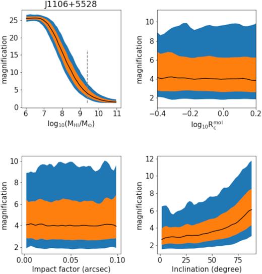
A selection of bivariate relations obtained from 104H i lensing simulations of the J1106+5228 lensing system. In each panel, the black curve shows the expectation, while the orange and blue filled areas show the 68 and 95 per cent confidence intervals, respectively. Upper left: magnification as a function of MH i. The grey, dashed vertical line presents the mass prediction from Maddox et al. (2015) stellar-H i mass relation. In this panel MH i was sampled from a uniform distribution (i.e. no PDF), however, in the other panels MH i was sampled from the optical prior. The MH i-magnification coupling is a direct result of equation (3). Upper right: magnification as a function of |$R_{\rm c}^{\rm mol}$|, showing no correlation is apparent over this range of parameters. Lower left: magnification as a function of impact factor for the range of impact factors as estimated from the HST model, showing this is indeed a nuisance parameter in this particular analysis. Lower right: magnification as a function of inclination, an increase in magnification is evident as the source becomes increasingly inclined. See main text for further detail on Monte Carlo assumptions, particularly on chosen parameter distributions and the justifications thereof.
To incorporate orientation effects, for each realization, the two-dimensional disc is simulated, and then randomly rotated in a three-dimensional cube to sample the inclination and position angles of the H i disc. The position angle is sampled uniformly over the range [0, 2π]. The inclination angle i is sampled with a probability density function (PDF) of sin (i) over the range [0, π/2].
We sample |$\log _{\rm 10}(R^{\rm c}_{\rm mol})$| from a normal distribution with [mean, stdev] = [−0.1, 0.3]. This is consistent with the range of |$M_{\rm H_2}/M_{\rm H\,{\small I}}$| quoted in Catinella et al. (2018) for the stellar mass range of these galaxies.
For the lens, the Einstein radius is sampled from a Gaussian distribution. The ellipticity and position angle of the lens is set to that of the observed optical distribution.
3.2.3 Dependence of free disc parameters on magnification
In order to understand the dependence of the magnification on the source parameters. We calculate H i magnifications for 104 random samples of the model and calculate the cumulative probability density function (CDF) of μ for each parameter individually, marginalized over the remaining parameters. These marginalized functions are computed numerically using a Monte Carlo integrator, which we use for a non-parameteric estimation of the expectation and confidence intervals, as shown in Fig. 4 for J1106+5228, Fig. A1 for J1250-0135 and Fig. A2 for J1143-0144.
To determine the PDF of μ(MH i), we marginalize over the other free parameters. This is the only function which we need and it requires no PDF for MH i (in other words, the PDF of μ is calculated at each MH i). This is presented in the upper-left panel of Fig. 4 and exhibits a tight relation between the average magnification and the H i mass which arises from equation (3). As the magnification is almost completely dependent on the mass, we can calculate a simplified conversion between H i mass and integrated H i flux.
To calculate the dependence of μ on the other disc parameters, we marginalize over MH i by sampling from the PDF predicted from the optical prior.
3.3 Probability distribution of H i mass
We now describe a mathematical model to evaluate the H i mass probability distribution, given an estimate of the integrated source flux and noise. This is a simplified model in which the measured integrated flux is solely attributed to Gaussian noise and lensed H i emission.
We do not assume that a detection has been made. Instead we attempt to answer the question: What is the probability distribution of real integrated flux (i.e. that is not due to noise) and associated mass? The equations are generally true for a measurement of a quantity S, given an integrated signal S0 with Gaussian noise. Importantly, we define ‘signal’ as the integrated flux, irrespective of a ‘detection’, hence the signal can be lower than the noise and even negative. In the case of pure noise, the expectation of the measured integrated flux is |$\langle$|S0|$\rangle$| = 0. If there is a true signal (even if it is smaller than the noise σS), |$\langle$|S0|$\rangle$| becomes positive. However, if S0/σS is small (as in two of our galaxies), the PDF of equation (5) will still have its expectation at S0, but with a large uncertainty that accounts for a significant probability of there being no true signal.
In the presence of noise, common objects (e.g. low-mass H i galaxies) can be mistaken as rare objects (e.g. high-mass H i galaxies) and vice versa. However, as there are more common objects, the number of common objects being mistaken for rare objects is larger than the reverse case. This leads to an overestimation of the number of rare objects. This is known as the Eddington bias (Eddington 1913). Given the asymmetric, declining H i mass function (HIMF) and symmetric Gaussian noise, it is much more likely that a source of measured integrated H i flux S0 has a true integrated flux smaller than S0 and a positive measurement error than vice versa.
Another way of understanding this is to consider a random sample x = log (M) drawn from a steep (i.e. highly asymmetric) mass function ρ(x). Then perturb x by a random error drawn from a Gaussian. Over many samples, these random errors systematically move the mass function towards the high-mass end. This is an important systematic effect, whenever the mass function changes significantly over the uncertainty of the mass measurement.
As physical considerations do not permit MH i to be negative, C0 should be interpreted as the probability of zero integrated H i flux.
The de-biased cumulative probability ΦEdd(MH i) (along with 68 per cent and 95 per cent confidence intervals) and the PDF of the H i mass derived from the stellar mass is shown in Fig. 5. Where applicable, the expectation of the de-biased mass as well as the boundaries of the confidence intervals is given in Table 1.
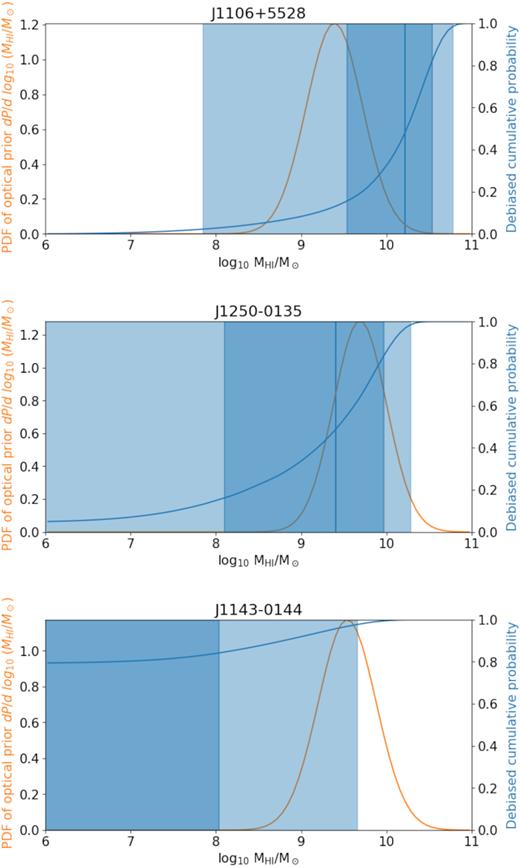
H i mass probability density functions for the three observed sources. The probability density as predicted by the Maddox et al. (2015) stellar mass –H i mass correlation is shown with orange curve. The Eddington-bias corrected (HIMF prior), cumulative probability ΦEdd(MH i) is shown by the blue curve. The 68 per cent and 95 per cent confidence intervals of ΦEdd(MH i) are shown with dark and light blue shading, respectively. The vertical blue line shows the expectation of the H i mass.
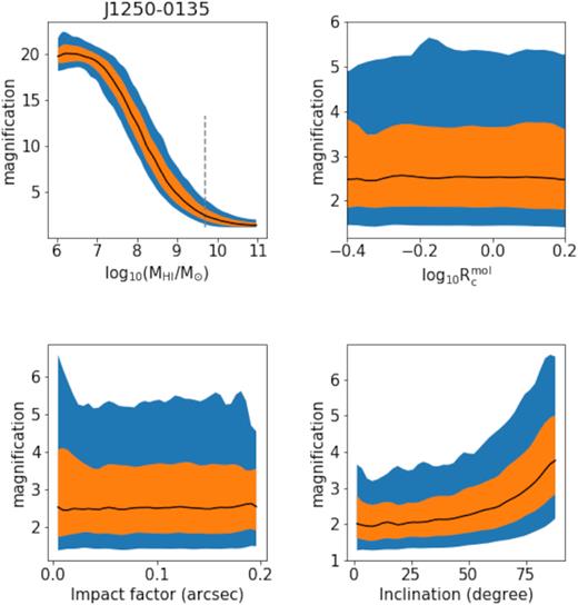
A selection of bivariate relations obtained from 104H i lensing simulations for the J1250−0135 galaxy–galaxy lens. In each panel, the black curve shows the expectation, while the orange and blue filled areas show the 68 and 95 per cent confidence intervals, respectively. Upper left: magnification as a function of MH i. The grey, dashed vertical line presents the mass prediction from Maddox stellar–H i mass relation. In this panel MH i was sampled from a uniform distribution, however, in the other panels MHI was sampled from the predicted mass probability density. Upper right: magnification as a function of |$R_{\rm c}^{\rm mol}$|, showing no correlation is apparent over this range of parameters. Lower left: magnification as a function of impact factor for the range of impact factors as estimated from the HST lens model. Lower right: magnification as a function of inclination. See main text for further detail on Monte Carlo assumptions, particularly on chosen parameter distributions and the justifications thereof.
4 DISCUSSION
4.1 H i mass constraints
Our Bayesian formalism aims to extract the maximum amount of information possible from the radio measurement. This is achieved by leveraging the optical spectroscopic information, correcting for Eddington bias and folding in a physical model of the magnification. The final product is the cumulative mass probability distribution along with non-parametric uncertainties. We emphasize that, these results apply only to the sampled 200 km s−1 (rest frame) bin centred on the best estimate of the source frequency position (see Section 2.3) and relate to the total H i mass of the galaxy as far as this bin contains the majority of the H i flux. In the event of unsampled flux, these results would underestimate the total H i mass and, on average, shift the cumulative probability ΦEdd(MH i) to lower masses.
We report evidence suggesting a marginal (3.8σ) H i detection for the lensed galaxy J1106+5228 (z = 0.4073) offset by 65 km s−1 from the optical redshift. We estimate the intrinsic mass integrated over 200 km s−1 (rest frame) at |$\log _{\rm 10} (M_{\rm H\,{\small I}}/M_\odot) = 10.2^{+0.3}_{-0.7}$| within the 68 per cent confidence interval. This estimated mass range is consistent with the stellar-mass prediction (see Fig. 5).
For all three sources, we do not find unambiguous detections at the expectation of the optical redshift but still extract information on MH i. For J1250−0135, we estimate |$\log _{\rm 10} (M_{\rm H\,{\small I}}/M_\odot) = 9.4^{+0.6}_{-1.3}$| within a 68 per cent confidence interval. This is consistent with the optical prediction. For J1143−0144 we obtain a 2σ upper limit of log10(MH i/M⊙) = 9.7 (see Table 1 for the full results).
In this paper, we have estimated that the source can be well-sampled by a Gaussian of FWHM ∼ 6 arcsec over a 200 km s−1 frequency interval. However, the physical size of the H i disc is dependent on the H i mass (Wang et al. 2016) and the frequency range is dependent on the inclination and total galaxy mass (McGaugh et al. 2000). Future analyses could be improved by a more detailed sampling of the integrated flux as a function of intrinsic mass and inclination.
The only previously published upper limit on integrated lensed H i flux (Hunt et al. 2016) placed competitive 3σ MH i upper limits of 6.58 × 10⁹ M⊙ at z = 0.398 and 1.5 × 10¹⁰ M⊙ at z = 0.487, however the assumption was made that the H i magnification is equal to the optical magnification which is inconsistent with our simulations (see next section). Their method constrains the H i mass by taking a factor of the spectral RMS as an upper limit on the lensed H i signal. We compare the 3σ (99.7 per cent confidence) limits derived by the two methods in the bottom two rows of Table 1. One difference is that in our model, the upper limits are a monotonically increasing function of the source-centred integrated flux. This implies that even negative integrated flux contains information about the possible source mass by lowering the H i mass upper limits as in the case of J1143−0144.
4.2 The H i magnification factor
For all three systems, the magnification is strongly dependent on the H i mass and the relation follows a reversed-‘S’ shape curve (see Fig. 4 upper left panel). On the low-mass end, the magnification converges to that of a point source (similar to the optical magnification) and on the high-mass end the magnification converges to 1. Between these extremes, the H i magnification is a monotonically decreasing function of H i mass. This is because the H i mass-size relation is monotonically increasing and the magnification is approximately equal to the ratio of lensed-to-intrinsic angular size.
Comparing the H i magnifications at the optically predicted H i mass with the optical magnifications (see Table. 1), we see that the H i magnifications are predicted to be significantly lower than the optical magnifications by a factor ∼3−7. The general trend of lower H i magnifications is due to H i being more extended than the stellar component. In practice, this effect should be heightened for these optically selected lensed systems which are biased towards compact nebular line emission components. Moreover, the effect is enhanced at these intermediate redshifts given the large H i source size-to-Einstein radius ratio.
As H i is more extended, the dependence of the magnification on sub-arcsecond offsets of the source centroid is significantly reduced. This point is illustrated in Fig. A2 (upper left panel), where there is only significant fluctuation in the magnification due to changes in the impact factor at very small masses (i.e. small sizes). This implies that the H i magnifications should not be approximated by the optical magnification but must be modelled separately. Note that this is not seen for the other two objects as the impact factor ranges were estimated to be closer to zero.
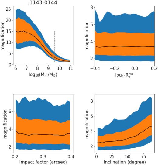
A selection of bivariate relations obtained from H i lensing simulations for the J1143−0144 galaxy–galaxy lens. See the caption of Fig. A1 for more details.
4.3 Considerations for future observations and surveys
Our results suggest that at a redshift of z ∼ 0.4, there is potential for using targeted observations of strong lenses with Einstein radii on the order of ∼1−2 arcsec to push the highest redshift H i detection threshold, as J1106+5228 would be if confirmed. However, due to the decreasing magnification boost as mass increases (see Fig. 4), we exclude the scenario of a large mass coupled with a high magnification. Again, these statements are only valid for SLACS-selected lenses at these intermediate redshifts for ∼1 arcsec-scale Einstein radii.
Strong lenses will however become increasingly important to consider for future H i surveys. There are several factors to consider. First, as the source redshift increases the lensing optical depth increases (i.e. more sources are lensed). For a velocity-integrated H i flux cut of 1.0 mJy km s−1, the fraction of lensed galaxies out of all galaxies will increase by a roughly 2–3 orders of magnitude from z ∼ 0.4 to z ∼ 2 (Deane et al. 2015). Secondly, the high end of the H i mass function might move to smaller masses with increasing redshift (Lagos et al. 2011) which by equation (3) would mean smaller intrinsic sizes and hence higher magnifications. Thirdly, the angular scale increases from approximately 5 kpc arcsec−1 to approximately 8 kpc arcsec−1, which is an effective decrease of about 2.5 in solid angle of the source, increasing magnification significantly for all source masses.
5 CONCLUSIONS AND FUTURE WORK
This work presents the first targeted interferometric observations of strongly lensed H i in emission, as well as the first detailed predictions of integrated H i flux magnification in individual galaxy–galaxy lensing systems. We have also developed a Bayesian formalism to estimate the H i mass probability density functions for all sources, even the clear non-detections. The spectrum of source J1106+5228 shows evidence of a marginal detection and is therefore an excellent candidate for follow up observations.
In the theory component of this work, we show that for this class of lensing system, the H i magnification is a monotonically decreasing function of H i mass because the H i mass–size relation is monotonically increasing. There is also saturation at low mass as the disc approximates a point source and at high mass where the disc is much larger than the Einstein radius.
The H i lensing simulation toolkit presented here allows for realistic feasibility studies for planning observations of H i in galaxy–galaxy lenses. We continue this lensed-H i campaign with both the upgraded-GMRT and the MeerKAT telescopes (Deane, Obreschkow & Heywood 2016).
In future, we look to extend the analysis to include cluster lenses as well as the statistics of lensing in cosmological volumes which would predict the effect of H i lensing on next-generation SKA surveys and the observed H i mass function, with particular reference to blind H i lens selection.
ACKNOWLEDGEMENTS
We thank Natasha Maddox and Julia Healy for discussions on alignment of the optical and H i signals in the frequency domain. We thank Gyula Jozsa for conversations on H i science. We also thank Benjamin Hugo, Kshitij Thorat, Sphesihle Makhathini, Jonathan S. Kenyon, and Oleg Smirnov for advice on interferometric data reduction. We thank Andre Offringa for help with using the wsclean software. This research was supported by the South African Radio Astronomy Observatory, which is a facility of the National Research Foundation, an agency of the Department of Science and Technology.
Footnotes
Specifically, we used a linear interpolation for the M⋆−MH i correlation presented in table 1 in Maddox et al. (2015) for the case which excluded galaxies without SDSS spectra.
Although, the stellar mass function changes significantly from z ∼ 0 to z ∼ 0.4 (Hopkins & Beacom 2006), the H i mass function is predicted to stay the same (Obreschkow & Rawlings 2009a; Lagos et al. 2011). Therefore, the general trend of the redshift evolution should be towards larger gas reservoirs at a given stellar mass.
Detection thresholds for H i sources coincident with optical sources should be set lower than the detections thresholds for a blind survey as the search space is vastly reduced and hence one is less likely to find rare noise spikes.
REFERENCES
APPENDIX A: EXTENDED SIMULATION RESULTS
We present the simulation results for sources J1250−0135 and J1143−0144 as described in Section 3.2. While the current observations of these targets do not share the heightened interest of a possible marginal detection as is the case with J1106+5228, the trends illustrate some of the relevant caveats to be considered in H i lensing, particularly for these low-to-intermediate redshifts.
