


ABSTRACT
X-ray observations of bright AGNs in or behind galaxy clusters offer unique capabilities to constrain axion-like particles. Existing analysis technique relies on measurements of the global goodness of fit. We develop a new analysis methodology that improves the statistical sensitivity to ALP–photon oscillations by isolating the characteristic quasi-sinusoidal modulations induced by ALPs. This involves analysing residuals in wavelength space allowing the Fourier structure to be made manifest as well as a machine learning approach. For telescopes with microcalorimeter resolution, simulations suggest these methods give an additional factor of 2 in sensitivity to ALPs compared to previous approaches.
1 INTRODUCTION
ALP–photon conversion is enhanced by large magnetic field coherence lengths. As it extends over megaparsec scales and contains coherence lengths up to tens of kiloparsecs, this makes the intracluster medium of galaxy clusters particularly efficient (Burrage, Davis & Shaw 2009; Horns et al. 2012; Conlon & Marsh 2013; Angus et al. 2014; Powell 2015; Conlon, Marsh & Powell 2016; Schlederer & Sigl 2016). This has allowed the use of X-ray point sources, located in or behind clusters, to produce leading bounds on ALP parameter space (Wouters & Brun 2013; Berg et al. 2017; Conlon et al. 2017; Marsh et al. 2017; Chen & Conlon2018; Conlon et al. 2018). While X-rays are particularly good at probing ALPs with |$m \lesssim 10^{-11} \, {\rm eV}$|, more massive ALPs can be probed via gamma-ray astronomy – see Wouters & Brun (2012), Ajello et al. (2016), Payez, Cudell & Hutsemekers (2012), and Majumdar, Calore & Horns (2018) for some related work in different wavebands.
The aim of this work is to improve the theoretical tools available for the analysis of ALP–photon conversion, and in particular the statistical methodology used to analyse data. Existing approaches to bounding ALP–photon conversion involve, roughly, a comparison of the overall goodness of fit (as measured by the reduced χ2) of models with ALPs compared to models without ALPs. For sufficiently large ALP–photon coupling, models with ALPs lead to a bad fit.
However, this approach makes little use of the actual structure of ALP–photon conversion. While the precise form of ALP–photon conversion depends on the (unknown) magnetic field along the line of sight, there is a quasi-sinusoidal oscillatory structure that is common to all realizations of the magnetic field. The aim of this paper is to develop analysis techniques to isolate this structure, and thereby allow greater sensitivity to constraining ALPs. This development of improved statistical methods is also important in view of the launch over the next decade of microcalorimeter-based X-ray telescopes such as XARM and Athena; the use of an overall χ2 fit would then fail to take full advantage of the energy resolution provided by such instruments.
With an eye on the opportunities that will come from future satellites such as XARM and Athena, we focus on energies and parameter ranges that are applicable for the case of X-ray photons converting to ALPs within galaxy cluster magnetic fields. However, our methods are in principle not limited to this case and can also be used for other photon energies whenever oscillations are expected. A version of our code can be found online.1
2 STATISTICS OF ALP–PHOTON CONVERSION
This equation involves an averaging over polarization states. As current X-ray telescopes are not sensitive to polarization, and the orientation of the cluster magnetic fields is independent of any polarization properties of the initial photons and randomized over many different domains, this is physically justified. For any one domain, the precise value of ε will depend on B⊥, but in all cases ε is small. For X-ray telescopes with polarization sensitivity, these assumptions would need to be revisited.
Along a sightline through a cluster, the magnetic field undergoes many reversals. We can model the cluster magnetic field as a sequential series of domains, each differing in terms of direction and coherence length, with an overall field strength set by a radial falloff moving away from the centre of the cluster. As the field directions vary between each domain, the conversion amplitudes add incoherently. This allows us the total survival probability to be obtained by multiplying the survival probability for each domain (although note that for the simulated data we numerically solve the full transfer matrix for the conversion amplitude).2
We note that this model consists of separate sequential magnetic field domains, each with a different coherence length and magnetic field. A more accurate model would involve, instead of distinct domains, many different scales simultaneously present in the magnetic field. However, simulations of photon–ALP conversion in such cases do not show major qualitative differences from the case where the different scales are represented by separate sequential domains (Angus et al. 2014). As it is conceptually and calculationally much simpler, and does not appear to be too misleading, we shall therefore work with a magnetic field model of separate and sequential domains. We have tested that the simplified approach discussed above leads to very similar results as a full simulation of an initial state through a simulated turbulent magnetic field that does not make use of the single domain formula but recursively solves the linearized Schrödinger equation of Raffelt & Stodolsky (1988).
In this paper, we will always assume that the overall photon–axion conversion probability is very small (less than 10 per cent) and the equations used in this section are only valid in this limit. This is not a significant restriction – if it is not the case, then the more advanced techniques of this paper are unnecessary as a simple test such as an overall χ2 fit will already show that the ‘standard’ astrophysical fit fails to describe the data.
This survival probability modulates the arriving photon spectrum. We shall assume that we know the correct functional form of the original source spectrum of photons, which we denote as |$\mathcal {M}(\omega)$|. For the purpose of this paper, we shall take this as a featureless power law plus an Fe K α line, although for more complicated spectra, this may also need to include more emission and absorption lines at (known) atomic energies.
3 ALP SEARCH STRATEGIES
The oscillatory structure of the residuals described in equation (16) can be exploited using any of the following three strategies:
An analysis of the Fourier transformed data,
a sinusoidal fit to the data,
a machine learning approach.
The Fourier transform of the data set can be directly calculated using fast Fourier transform methods. As opposed to a fit, this does not require optimization of any of the parameters involved. Fitting to a small number of sinusoidal functions can be an efficient way to capture any oscillatory structure present in the residuals. The machine learning approach uses the complete list of residual data as an input to ‘learn’ from a training set what value of g is associated. Contrary to the Fourier and fit method, the machine learning method does not rely on the data being of oscillatory nature. It can be thought of as a universal fit: once the network is trained it includes all the relevant information that influence the conversion of photons to axions along the line of sight. Hence, it can be used as a benchmark for the Fourier and fit method: once those methods perform as well as the somewhat brute force machine learning approach, we know that we are able to resolve – and understand – all the possible structure of photon to ALP conversion imprinted on to the residuals.
In the following, we present the three methods in more detail, allowing a comparison between each of the three.
3.1 Analysis of Fourier-transformed data
The essence of the axion search is that we expect the axions to introduce modulations that allow this data to be well approximated by only its low-frequency Fourier modes, i.e. K ≪ M/2 (at least in the limit of a very large number of data points).
3.2 Sinusoidal fit
3.3 Machine learning
We set up a deep neural network (DNN) with Tensorflow 4 that uses the list of residuals |$\mathcal {F}_i$| in its entirety as ‘feature columns’ while the value of g that has been used to simulate those residuals is used as the ‘label column’. The design parameters of the DNN are the number of layers and the number of nodes as well as the loss function that the network tries to optimize. For the loss function, we use the sum of squared errors between the actual and the DNN predicted values of the residuals |$\mathcal {F}_i$|. The data are shuffled and divided into a training (75 per cent of data) and a test set (25 per cent of data). The training data is used to teach the network which value of g is associated to a list of residuals by optimizing the parameters of each node while the test data is used to test how well the DNN performs and to estimate the prediction error. The data contain a sample of different realizations of the magnetic field model and Poisson errors. Hence, the DNN does not learn the residual structure for a particular realization of the magnetic field but its marginalized statistical properties. The number of layers and nodes are chosen such that the difference between the test error and training error is minimized, i.e. the network is built with enough flexibility to capture the data but avoids overfitting. We try one, two, and three layers and vary the number of nodes in steps of 10. Examining the training and test error, we find the optimal value to be at two layers and 200 (40) nodes for Athena (XMM). Three layers generally lead to overfitting even for a small number of nodes.
4 ALP DATA SIMULATION
We now aim to test this method on simulated data for XMM–Newton and Athena. Our focus here is on comparison of this method to a pure overall χ2 fit (and hence whether it is possible to improve statistical sensitivity), rather than on applications to any particular real data set or to precise forecasts of future telescope sensitivity.
As one of the most promising targets for ALP–photon conversion is the central Perseus AGN NGC 1275, we let ALP represent simulated survival probabilities for the Perseus cluster environment, i.e. for ALP–photon conversion within an electron density ne and magnetic field model representing that of the Perseus cluster. As the B-field properties can only ever be known statistically, and each explicit realization leads to different conversion probabilities even for statistically identical B-field parameters, we need to marginalize over many realizations of the magnetic field in Perseus.
Based on XMM–Newton pn and predicted Athena XIFU responses,5 we generate fake data using the xspec command fakeit with a simulated exposure time of 500 ks. fakeit simulates Poisson errors based on the exposure time. In terms of fitting, we work with an energy interval between 1.5 and 4.5 keV for XMM–Newton and from 0.7 to 1.4 keV for Athena. This allows the demonstration of the ability of Athena (or any other telescope with microcalorimeter level resolution) to resolve the rapid ALP-induced oscillations that would be present at lower energies. For a real data set, one would of course use the full energy range of the telescope.
We now describe the methods used to analyse the fake data sets:
- We first fit a zero modelspectrum to the data. The ALPGlob component represents the global modulation due to ALPs given in (13) and is given as(32)\begin{eqnarray*} wabs * ALPGlob * (zpowerlw + zgauss) \end{eqnarray*}where |$A = \omega _0^{-2} \sum \epsilon _i$|.(33)\begin{eqnarray*} ALPGlob = 1- A\, \omega ^2\, , \end{eqnarray*}
In the absence of ALPs, one would expect the best-fitting value of A to vanish. In the presence of ALPs, while such a term removes the ‘global’ effects it will not account for the oscillations contained within the ALP component in (29). Hence, for a strong axion–photon coupling |$\chi _0^2/$|dof would be significantly larger than one.
- We perform a Fourier analysis (as described in Section 3.1) and a sinusoidal fit (as described in Section 3.2) of |$(x_i,y_i) = \left(\omega _i^{-1},\omega _i^{-2}\mathcal {F}(\omega _i)\right)$| for a given K.6 If low mode oscillations are present in the data, thenper dof will improve significantly compared to |$\chi _0^2$|. The function y(ω) equals y(K)(ωi) for the Fourier method and |$y^{(N_{\text{fit}})}(\omega _i)$| for the sinusoidal fit.(34)\begin{eqnarray*} \chi _1^2 & = & \sum _{i=1}^N \frac{\left[ \mathcal {F}(\omega _i) - \omega _i^2\, y(\omega _i) \right]^2 }{\sigma _i^2} \end{eqnarray*}The Fourier function y(K)(ω) generally overestimates the fluctuations in the simulated data |$\omega _i^{-2}\mathcal {F}(\omega _i)$| at the edges of the energy intervals. This is particularly significant for XMM data where the residuals are often constant for large ω ≲ 4.5 keV while y(K)(ω) can oscillate strongly. This would lead to a bad fit to the data which is why we use a smoothing function S(ω) that multiplies y(K)(ω) to smooth it out at the edges of the energy interval. For the Fourier method only, |$\chi _1^2$| is then calculated aswhere we choose S(ω) = 1keV2/ω2 as a smoothing function.7(35)\begin{eqnarray*} \chi _{1,\text{Fourier}}^2 & = & \sum _{i=1}^N \frac{\left[ \mathcal {F}(\omega _i) - \omega _i^2\, S(\omega _i)\, y^{(K)}(\omega _i) \right]^2 }{\sigma _i^2}\, , \end{eqnarray*}
The DNN is fitted by using 75 per cent of the residuals |$\mathcal {F}_i$| as training data. For the remaining 25 per cent of the residual data set the DNN predicts the value of g.
We show in Fig. 1 how low Fourier modes can capture residuals in the data, for XMM–Newton and Athena, respectively. The values of Nfit and K are chosen such that the low Fourier mode oscillations in the data can be accommodated. For this purpose, we examine plots such as Fig. 1 for different realizations of the magnetic field model and check how many Fourier modes we need to include to represent the oscillatory structure. Since Athena has a much better energy resolution than XMM–Newton, it can resolve a higher number of high-frequency modes.
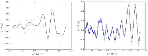
For particular B-field and Poisson error realizations, we show plots of residuals |$y_i = \omega _i^{-2}\mathcal {F}(\omega _i)$| versus low mode sinusoidal fit function |$y_{\text{fit}}^{(8)}$| for XMM (left side), and versus Fourier decomposition y(16) for Athena (right side) as a function of inverse energy. The ALP to photon coupling is |$g = 5 \times 10^{-12} \, {\rm GeV}^{-1}$|.
Photon to ALP modulations are very well represented by the leading Fourier modes and hence this analysis is very sensitive to the presence of ALP physics. An atomic line for instance would lead to virtually no improvement in Δχ2(g) when using a Fourier analysis and hence would not be picked up by our method. The method is also very efficient as the calculation of Fourier coefficients can be performed very quickly and no spectral fit beyond the standard absorbed power law is necessary.
Note that Δχ2(g = 0) represents improvements in the fit due simply to Poisson noise – even in the absence of ALPs. It is expected that some improvement can be attained by fitting the Poisson noise of the residuals with sinusoidal functions. Constraints will be obtained when Δχ2(g) ≫ Δχ2(g = 0).
For every g, we generate 40 realizations of the magnetic field in Perseus and subsequently 50 fake data sets with different Poisson errors. Hence, for every g there are 2000 sets of simulated data.
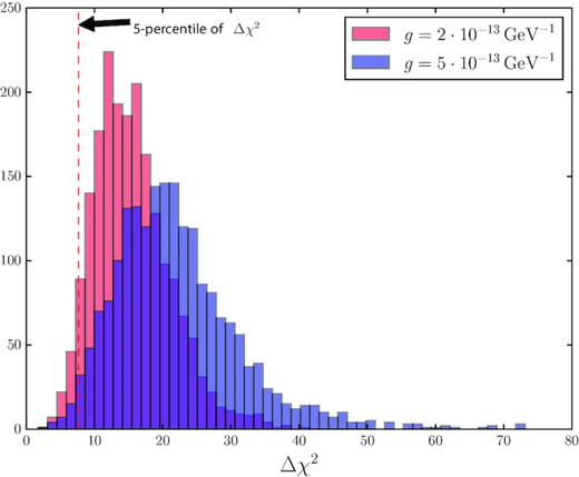
Histogram of the Δχ2 distributions for |$g = 2 \times 10^{-13} \, {\rm GeV}^{-1}$| (red) and |$g = 5 \times 10^{-13} \, {\rm GeV}^{-1}$| (blue). As g increases the distribution moves towards larger Δχ2. The red dotted line shows the 5th percentile of the Δχ2 distribution for |$g = 2 \times 10^{-13} \, {\rm GeV}^{-1}$|. The 5th percentile of the simulated data is used to infer a bound on g, see main text. This plot uses the sinusoidal fit method for XMM–Newton simulated data.
5 RESULTS
In the following, we compare the standard |$\chi ^2_0$| calculation that was previously used to look for ALPs to the Fourier method explained in Section 3.1, the sinusoidal fit method explained in Section 3.2, and the machine learning approach discussed in Section 3.3. We apply these methods to the simulated data for XMM and Athena.
5.1 Athena
The standard power law |$\chi ^2_0$| method, the weighted Fourier method, the sinusoidal fit method, and the DNN machine learning method are shown in Fig. 3. Every data set contains ∼1800 points so for small g < 10−13 GeV−1 where the power law is already a decent fit to the data, we expect a |$\chi _0^2 \sim 1800$| which is what we find. Once we rebin two data points to one for the Fourier and fit method, the degrees of freedom are roughly divided by two so |$\chi _0^2(\text{Fourier,Fit}) \sim 900$|. |$\chi _1^2$| is calculated once the Fourier modes or the sinusoidal fit function are included. Even for very small g, we expect these methods to slightly improve the fit, hence |$\chi _1^2 \lt \chi _0^2$|, effectively fitting Poisson noise. We find |$\chi _1^2 \lesssim \chi _0^2$| for very small g < 10−13 GeV−1 as expected. We examine the coverage of all four methods using our simulation data and find that while the |$\chi ^2_0$| method generally gives the right coverage for all values of g the other three methods give undercoverage for small values of g ≲ 2 |$\times$|10−13 GeV−1 and overcoverage for g ≳ 2 |$\times$| 10−12 GeV−1. In the intermediate range, the method gives the right coverage. As large values of g are already excluded and small values of g are below the 95 |${{\ \rm per\ cent}}$| limit of the methods and hence below the discovery potential of the instrument, the intermediate range is the only one that is practically relevant.
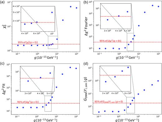
The four results for Athena. From left to right, top to bottom, these plots show (a) 5 percentile of the power-law fit |$\chi _0^2(g)$| for Athena. There are 1747 degrees of freedom for this fit. The dashed red line is the 95th percentile of |$\chi ^2_0 (g=0)$| and marks which values of g can be excluded: a point above it can be excluded at 95 per cent confidence. (b) 5 percentile of Δχ2(g) for the Fourier method with ω−2weighting (see the text) and K = 16 for Athena. (c) 5 percentile of Δχ2(g) for a sinusoidal fit with Nfit = 16 for Athena. (d) 5th percentile of |$G_\text{DNN}(\mathcal {F}_{i,\text{sim}}\, |\, g)$| for the DNN method for Athena. The dashed red line is the 95th percentile of |$G_\text{DNN}(\mathcal {F}_{i,\text{sim}}\, |\, g=0)$| and marks which values of g can be excluded: a point above it can be excluded at 95 per cent confidence.
As illustrated in these figures, the |$\chi ^2_0$| method gives a bound of g ≲ 5.9 |$\times$| 10−13 GeV−1. The weighted Fourier method and the fit method do significantly better with a bound of g ≲ 3.8 |$\times$| 10−13 GeV−1. The DNN method also does better giving a bound of g ≲ 4.2 |$\times$| 10−13 GeV−1. This represents an improvement by a factor of 1.5 in the coupling compared to the |$\chi ^2_0$| method. As all actual physical effects (interconversion of photons and axions) scale as |$g_{a \gamma \gamma }^2$|, the improvement in sensitivity is then slightly greater than a factor of 2.
5.2 XMM–Newton
The results for XMM–Newton are all shown in Fig. 4. In this case, the sinusoidal fit method can exclude g between 5 |$\times$| 10−13 GeV−1 and 10−12 GeV−1 and hence does slightly better than the |$\chi ^2_0$|, weighted Fourier and DNN methods which can only exclude g > 10−12 GeV−1. Again, we check for coverage and find the same result as for Athena: the relevant intermediate range of g has the right coverage while there is undercoverage for small values and overcoverage for large values.
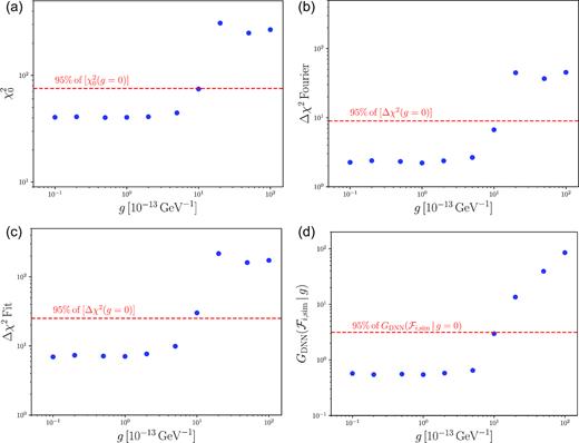
The four results for XMM. From left to right, top to bottom, these plots show (a) 5th percentile of the power-law fit |$\chi _0^2(g)$| for XMM. There are 56 degrees of freedom for this fit. The dashed red line is the 95th percentile of |$\chi ^2_0 (g=0)$| and marks which values of g can be excluded: a point above it can be excluded at 95 per cent confidence. (b) 5th percentile of Δχ2(g) for the Fourier method with ω−2 weighting (see the text) and K = 8 for XMM. (c) 5th percentile of Δχ2(g) for a sinusoidal fit with Nfit = 8 for XMM. (d) 5th percentile of |$G_\text{DNN}(\mathcal {F}_{i,\text{sim}}\, |\, g)$| for the DNN method for XMM. The dashed red line is the 95th percentile of |$G_\text{DNN}(\mathcal {F}_{i,\text{sim}}\, |\, g=0)$| and marks which values of g can be excluded: a point above it can be excluded at 95 per cent confidence.
6 DISCUSSION
X-ray observations of AGNs offer one of the most sensitive probes of axion-like particles in the low-mass regime and it is therefore important to ensure that maximal statistical sensitivity is obtained in searches for them. In this paper, we have developed analysis methods aimed at exploiting the characteristic quasi-sinusoidal modulations that are induced by ALPs. Based on simulated data, these methods appear to improve sensitivity to photon–axion conversion by a factor of 2 (in conversion probability).
SUPPORTING INFORMATION
Supplementary data are available at https://github.com/mrummphys/axion_statistics online.
Please note: Oxford University Press is not responsible for the content or functionality of any supporting materials supplied by the authors. Any queries (other than missing material) should be directed to the corresponding author for the article.
ACKNOWLEDGEMENTS
We thank Cliff Burgess, Francesca Day, Nicholas Jennings, Sven Krippendorf, David Marsh for discussions. This work was funded in part by ERC Starting Grant 307605.
Footnotes
Although the axion propagation equations evolve amplitude not probability, it is the fact that different domains add incoherently that makes it sufficient to combine probabilities across domains.
For example, see https://www-user.tu-chemnitz.de/ potts/nfft/.
We use the DNNRegressor estimator. For more details, see the Tensorflow documentation.
These are taken from https://www.cosmos.esa.int/web/xmm-newton/epic-response-files and www.cfa.harvard.edu/jzuhone/soxs/responses.html.
For Athena data, we rebin two data points to one data point to speed up the calculation as half the energy resolution of Athena is easily sufficient to resolve ALP modulations.
We have tried different powers of ω as smoothing functions and found that ω−2 has the desired effect as it smooths along the edges but does not suppress too much structure in the bulk of the given energy range.
