


ABSTRACT
We present a detailed exploration of the stellar mass versus gas-phase metallicity relation (MZR) using integral field spectroscopy data obtained from ∼1000 galaxies observed by the SAMI galaxy survey. These spatially resolved spectroscopic data allow us to determine the metallicity within the same physical scale (Reff) for different calibrators. The shape of the MZ relations is very similar between the different calibrators, while there are large offsets in the absolute values of the abundances. We confirm our previous results derived using the spatially resolved data provided by the CALIFA and MaNGA surveys: (1) we do not find any significant secondary relation of the MZR with either the star formation rate (SFR) or the specific SFR (SFR/M*) for any of the calibrators used in this study, based on the analysis of the individual residuals; (2) if there is a dependence with the SFR, it is weaker than the reported one (rc ∼ −0.3), it is confined to the low-mass regime (M* < 109 M⊙) or high-SFR regimes, and it does not produce any significant improvement in the description of the average population of galaxies. The aparent disagreement with published results based on single-fibre spectroscopic data could be due to (i) the interpretation of the secondary relation itself; (ii) the lower number of objects sampled at the low-mass regime by the current study; or (iii) the presence of extreme star-forming galaxies that drive the secondary relation in previous results.
1 INTRODUCTION
Metals are the product of thermonuclear reactions that occur as stars are born and die. They enrich the gas in the interstellar medium, where the enrichment is modulated by gas inflows and outflows. Observationally, gas-phase oxygen abundance has the largest importance, as the most frequent metal element. Oxygen is mostly created by core-collapse supernovae associated with star formation events. It produces strong emission lines in the optical wavelength range when ionized and it is a particularly good tracer of the abundance in the inter-stellar medium. Therefore, it is a key element to understand the matter cycle of stellar evolution, death, and metal production.
For these reasons, oxygen has been used as a probe of the evolution of galaxies. For example, the presence of a negative oxygen abundance gradient in spiral galaxies (Searle 1971; Comte 1975) and the Milky Way (Peimbert, Torres-Peimbert & Rayo 1978), recurrently confirmed with updated observations using larger surveys of galaxies (e.g. Sánchez et al. 2013; Sánchez-Menguiano et al. 2016, 2018; Belfiore et al. 2017) and H ii regions in our Galaxy (e.g. Esteban & García-Rojas 2018), is one of the key pieces of evidence for the inside-out scenario of galaxy growth (e.g. Matteucci & Francois 1989; Boissier & Prantzos 1999). Several different scaling relations and patterns have been proposed between the oxygen abundance and other properties of galaxies, like (i) the luminosity (e.g. Lequeux et al. 1979; Skillman 1989), (ii) the surface brightness (e.g. Vila-Costas & Edmunds 1992; Zaritsky, Kennicutt & Huchra 1994), (iii) the stellar mass (e.g. Tremonti et al. 2004; Kewley & Ellison 2008), and (iv) the gravitatinal potential (D’Eugenio et al. 2018). Some properties derived from the abundance, like the effective yield, correlate with global properties of galaxies too (e.g. Garnett 2002). Beyond the integrated or average properties of galaxies, the spatially resolved oxygen abundances also present scaling relations with the local surface brightness (e.g. Pilyugin et al. 2014) and the stellar mass density (e.g. Rosales-Ortega et al. 2012; Barrera-Ballesteros et al. 2016). All of them provide strong constraints on how galaxies evolve, connecting different products of stellar evolution, like stellar mass and luminosity, or tracers of the dynamical stage, like velocity and gravitational potential, with oxygen abundance.
A particularly important relation is the mass–metallicity relation (MZ-relation), since it connects the two main products of stellar evolution. This relation has been known for decades (e.g. Vila-Costas & Edmunds 1992); however, it was not explored in detail using a statistically significant and large sample until more recently: Tremonti et al. (2004, T04 hereafter) show that these two parameters exhibit a tight correlation with a dispersion of ∼0.1 dex over ∼4 orders of magnitudes in stellar mass. This correlation presents a similar shape at very different redshifts (e.g. Erb et al. 2006; Erb 2008; Henry et al. 2013; Saviane et al. 2014; Salim et al. 2015), but shows a clear evolution that reflects the change of the two involved parameters with cosmic time (e.g. Moustakas et al. 2011; Marino et al. 2012). The relation also presents a very similar shape irrespective of the oxygen abundance calibrator, with an almost linear trend for M* < 1010 M⊙, and then a bend and flattening towards an asymptotic value for larger stellar masses (e.g. Kewley & Ellison 2008). On the other hand, the normalization and scale of the abundances depend strongly on the calibrator (e.g. Kewley & Ellison 2008; Barrera-Ballesteros et al. 2017; Sánchez et al. 2017). Finally, a similar shape is derived independently of whether single aperture or spatially resolved spectroscopic data are being used (e.g. Rosales-Ortega et al. 2012; Sánchez et al. 2014; Barrera-Ballesteros et al. 2017).
The MZ-relation presents two different regimes that are interpreted in a very different way. For the low-mass regime, the linear relation between the stellar mass and the oxygen abundance can be interpreted as the consequence of the star formation history in galaxies, without involving major dry mergers. Since both stellar mass and oxygen abundance are the consequence of star formation, both of them should grow in a consistent way, coevolving. Under the assumption of no inpflow/outflow of gas, the so-called closed-box, the chemical enrichment would be fully consistent with the integral of the star formation rate over cosmic times (star formation histories), and therefore a linear relation between oxygen abundance and stellar mass would be expected. It has been known for a long time that this simple enrichment model cannot reproduce the metallicity distribution in the disc of galaxies (e.g. Erb 2008; Belfiore, Maiolino & Bothwell 2016; Barrera-Ballesteros et al. 2018). Therefore, infall and leaking of gas is required (e.g. G-dwarf problem, Binney, Merrifield & Wegner 2000), as well as an equilibrium between in-/outflows and the reservoir of gas in galaxies (e.g. Matteucci 1986; Lilly et al. 2013).
At high masses, in the asymptotic regime, the gas metallicity seems to reach a saturation value independent of stellar mass. That saturation value depends on the adopted calibrator. T04 interpreted that saturation as a consequence of galactic outflows that regulate the metal content. A priori, it was assumed that outflows are stronger for galaxies with higher star formation rates, that are at the same time also the more massive galaxies (among those forming stars). This assumption seems to be confirmed observationally (Heckman 2001), despite the fact that the loading factor decreses with stellar mass too (e.g. Peeples & Shankar 2011). In this hypothesis, an equilibrium is reached between the oxygen production and the metals expelled by outflows (e.g. Davé, Finlator & Oppenheimer 2011; Lilly et al. 2013; Belfiore et al. 2016; Weinberg, Andrews & Freudenburg 2017). As outflows from galaxies are global processes, this interpretation requires that outflows affect the global metallicity in galaxies. A caveat would then be that outflows are more frequently found in the central regions of galaxies (e.g. López-Cobá et al. 2017, 2019).
Another interpretation not involving outflows is that the asymptotic value is a natural consequence of the maximum amount of oxygen that can be produced by stars, i.e. the yield. Irrespective of the inflows or outflows of gas, oxygen abundance cannot be larger than the theoretical limit of production of this element at a considered gas fraction (fgas). In the case of the closed-box model, metallicity is proportional to the yield times the natural logarithm of the inverse of fgas. Therefore, if all gas is consumed in a galaxy (fgas = 0), the oxygen abundance diverges, becoming infinite (in essence, not due to the production of more metals, but due to the lack of hydrogen). However, all galaxies with measured gas-phase oxygen abundance have a certain amount of gas, fgas clearly non-zero. Indeed, Pilyugin, Thuan & Vílchez (2007) show that the current asymptotic value is compatible with a closed-box model for a fgas ∼ 5–10 per cent. In the presence of gas flows, the asymptotic value would correspond to a different fgas, as the theoretical yield is modified by the corresponding effective one. In this scenario, metal enrichment is dominated by local processes, with a limited effect of the outflows and only requiring gas accretion to explain not only the global mass-metallicity relation by its local version, the so-called Σ*–Z relation (Rosales-Ortega et al. 2012; Sánchez et al. 2013; Barrera-Ballesteros et al. 2016), and even the abundance gradients observed in spiral galaxies (e.g. Sánchez et al. 2014; Sánchez-Menguiano et al. 2016, 2018; Poetrodjojo et al. 2018). The detailed shape of the MZ-relation is therefore an important constraint for the two proposed scenarios.
In the last decade, it has been proposed that the MZ-relation exhibits a secondary relation with the star formation rate (SFR), first reported by Ellison et al. (2008). This secondary relation was proposed (i) as a modification of the dependence of the stellar mass with a parameter that includes both this mass and the SFR (the so-called Fundamental Mass Metallicity relation, or FMR; Mannucci et al. 2010); (ii) as a correlation between the three involved parameters (the so-called Fundamental Plane of Mass-SFR-Metallicity, or FP; Lara-López et al. 2010); or (iii) as a correlation between the residuals (after subtraction of the MZ-relation) with either the SFR or the specific star formation rate, sSFR (Salim et al. 2014). This relation was proposed based on the analysis of single-fibre spectroscopic data provided by the Sloan Digital Sky Survey (SDSS; York et al. 2000).
The existence of this secondary relation is still debated based on the analysis of new integral field spectroscopic (IFS) data. The analysis of the data provided by the CALIFA survey (Sánchez et al. 2012) for a sample of 150 nearby galaxies did not find a secondary relation with the SFR (Sánchez et al. 2013). Hughes et al. (2013) found similar results with integrated values provided by a drift-scan observational setup. Also, T04 explored the residuals once subtracted from the MZ relation, and they did not find a dependency with the EW(|$\rm {H}\alpha$|), a tracer of the sSFR (e.g. Sánchez et al. 2013; Belfiore et al. 2017). This result has been confirmed using larger IFS data sets by Barrera-Ballesteros et al. (2017) and Sánchez et al. (2017). They used nearly ∼2000 galaxies extracted from the MaNGA survey (Bundy et al. 2015) and the updated data set of ∼700 galaxies provided by the CALIFA survey (Sánchez et al. 2012), respectively. More recent results, using single-aperture spectroscopic data, found that the presence of an additional dependence with the SFR strongly depends on the adopted calibrator, disappearing for some calibrators (e.g. Kashino et al. 2016), or being weaker than previously found (e.g. Telford et al. 2016). Re-analysis of the IFS data set by Salim et al. (2014) emphasized the complexity of providing the correct parameterization of the Mass–SFR–Metallicity plane, finding that the dependence on SFR is strongest for the galaxies with highest sSFR. Finally, the more recent published analysis using high-quality spatial resolved MUSE IFS data over a limited sample of galaxies confirms previous results based on spatial resolved information, without detecting a clear secondary relation with the SFR (Erroz-Ferrer et al. 2019)
In this work, we explore the MZ relation and its possible dependence on SFR using the IFS data extracted from the ongoing SAMI galaxy survey (Croom et al. 2012). The paper is distributed in the following sections: the sample of galaxies, a summary of the reduction and the overall data set used in this article are presented in Section 2; the analysis performed over this data set is described in Section 3, including a description of how the different involved parameters (stellar mass, star formation rate, and the oxygen abundance from different calibrators) are derived; a description of the Mass–Metallicity (MZ) relation for the analysed galaxies is presented in Section 4.1, exploring the proposed dependence with the SFR in Section 4.2; a detailed analysis of the Fundamental Mass–Metallicity Relation (Mannucci et al. 2010) and Fundamental Plane (Lara-López et al. 2010) are described in Section 4.4 and 4.5, respectively. The proposed dependence of the residuals after subtraction of the MZ-relation and removal of the dependence of the residuals of the SFR with stellar mass are included in Section 4.6. Section 5 includes the discussion of the results of all of these analyses, with a summary of the conclusions included in Section 6. Throughout this work, we assume the standard Λ Cold Dark Matter cosmology with the parameters: H0 = 71 km s−1 Mpc−1, ΩM = 0.27, |$\Omega _\Lambda$| = 0.73.
2 SAMPLE AND DATA
The selection of the SAMI galaxy survey sample is described in detail in Bryant et al. (2015), with further details in Owers et al. (2017). A comparison with the sample selection of other integral field spectroscopic surveys was presented in Sánchez et al. (2017).
In short, the SAMI galaxy survey sample consists of two separate sub-samples: (i) a sub-sample drawn from the Galaxy And Mass Assembly (GAMA) survey (Driver et al. 2011) and (ii) an additional cluster sample. The SAMI-GAMA sample consists of a series of volume-limited sub-samples, in which the covered stellar mass increases with redshift. It includes galaxies in a wide range of environments, from isolated up to massive groups, but it does not contain cluster galaxies. For this reason, a second sub-sample was selected, by selecting galaxies from eight different galaxy clusters in the same redshift foot-print of the primary sample (i.e. z ≤ 0.1) as described in Owers et al. (2017). A stellar mass selection criterion was applied to the cluster sample, with different lower stellar mass limits for clusters at different redshifts. Finally, a small sub-set of filler targets were included to maximize the use of the multiplexing capabilities of the SAMI instrument (Sharp et al. 2006; Bland-Hawthorn et al. 2011; Bryant et al. 2011; Croom et al. 2012).
The sample analysed here consists of a random sub-set of the foreseen final sample of SAMI targets (just over 3000 objects once the survey is completed). It comprises the 2307 galaxies observed by August 2017, included in the internal SAMI v0.10 distribution. These galaxies cover the redshift range between 0.005 < z < 0.1, with stellar masses between ∼107–1011.5 M⊙, and with an extensive coverage of the colour–magnitude diagram, as already shown in Sánchez et al. (2017). This sub-sample can be volume-corrected following the prescriptions described in Sánchez et al. (2018), finding that it is complete in the range between ∼108.5–1011.2 M⊙.
2.1 Data reduction
The data reduction is described in detailed in Allen et al. (2015) and Sharp et al. (2015), and it is similar to the one adopted for the SAMI DR1 Green et al. (2018) and DR2 Scott et al. (2018). We present here a brief summary.
The first steps of the reduction comprise the overscan subtraction, spectral extraction, CCD flat-fielding, fibre throughput and wavelength calibration and finally sky subtraction. The result of those steps is the standard RSS-frame (Sánchez 2006). These steps are performed using the 2dfDR data reduction package.1
Then, each RSS-frame is spectrophotometrically calibrated and corrected for telluric absorption. Finally, the resulting RSS-frames are combined into a 3D data cube by resampling them on to a regular grid, with a spaxel size of 0.5″ × 0.5″. This procedure involves a spatial registration of the different dithered positions, a correction of the differential atmospheric refraction, and final zero-point absolute flux recalibration. All these final procedures are performed using the SAMI Python package described in Allen et al. (2014). The final result of the data reduction is a single data cube for each observed target and each wavelength regime.
The SAMI observational setup uses the two arms of the spectrograph, one in the blue, covering the wavelength range between ∼3700 Å and ∼5700 Å with a resolution of ∼173 km s−1 (FWHM), and one in the red, covering the wavelength range between ∼6250 Å and ∼7350 Å, with a resolution of ∼67 km s−1 (FWHM). Therefore, the standard data-reduction produces two different data cubes, with two different wavelength ranges, spectral resolutions and spectral sampling. In this analysis, we combined those two data cubes into a single cube, following a similar procedure as that adopted for the CALIFA data cubes (e.g. Sánchez et al. 2016c), by (i) degrading the resolution of the red-arm (R ∼ 4300) data cubes to that of the blue-arm (R ∼ 1800), (ii) re-sampling the full spectra to a common sampling of 1 Å, and (iii) correcting them for Galactic extinction, using the attenuation curves provided by the SAMI data-reduction. The degradation and resampling of the spectra is required for our adopted analysis scheme (described below). The final data cubes cover a wavelength range between ∼3700 Å and ∼7350 Å, with a gap between ∼5700 Å and ∼6250 Å, in a homogeneous way in terms of spectral resolution. These cubes cover a wavelength range similar to the one covered by the V500 data cubes of the CALIFA survey (e.g. Sánchez et al. 2012), apart from the gap, with a resolution similar to that of the MaNGA data cubes (e.g. Law et al. 2015). The final format of this COMBO data cubes is similar to the one adopted for the cubes in the CALIFA galaxy survey (e.g. García-Benito et al. 2015). We make use of those COMBO data cubes in the current analysis, since we consider that they provide the best compromise between spectral resolution and largest wavelength coverage that can be provided by the SAMI data set. This is particularly important to optimize the removal of the stellar continuum in the best possible way before analysis of the stellar continuum. These combined data cubes would not be suitable for kinematic analysis.
The final spectrophotometric precision and accuracy of the analysed data were explored by Green et al. (2018). They state clearly that the accuracy of the photometry is of the order of 4 per cent, when compared to that of the SDSS imaging survey, with a typical precision of 10 per cent. This precision is slightly worse than that derived for other IFS surveys (3-4 per cent Sánchez et al. 2016c), however, is partially due to the lower S/N of the SAMI data in the continuum. A similar calculation for the SDSS itself indicates that for point-like sources the typical precision is of ∼4 per cent, without knowing the exact value for extended targets,2 although it is expected to be larger. This precision should not affect significantly any of the parameters analysed in the current study, as reported based on the comparison between different IFU surveys in Section 4. If any, it may increase the dispersion in the reported correlations, but not in a large way, as shown in the present work. From the original observed sample, we exclude 53 galaxies for which there was an obvious error in the spectrophotometric calibration between the blue and red arms, and/or they present an S/N clearly lower than the average. Due to the limited number of excluded galaxies, that exclusion should not affect the results.
3 ANALYSIS
The analysis of the data cubes was done making use of Pipe3D (Sánchez et al. 2016b), a pipeline designed to (i) fit the stellar continuum with synthetic population models and (ii) extract the information from the ionized gas emission lines of Integral Field Spectroscopy (IFS) data cubes. Pipe3D uses FIT3D algorithms as the basic fitting routines (Sánchez et al. 2016a).3 The adopted implementation of Pipe3D analyses the stellar populations by decomposing them using the GSD156 single stellar population (SSP) library. This library, first described in Cid Fernandes et al. (2013), comprises 156 SSP templates, that sample 39 ages (1 Myr to 14 Gyr, in an almost logarithm scale), and four different metallicities (Z/Z⊙ = 0.2, 0.4, 1, and 1.5), adopting the Salpeter Initial Mass Function (IMF Salpeter 1955). These templates have been extensively used in previous studies (e.g. Pérez et al. 2013; González Delgado et al. 2014; Ibarra-Medel et al. 2016; Sánchez et al. 2018). The degradation and resampling of the spectra described in the previous section was therefore mandatory since (i) the resolution of the adopted SSP library is worse than that of the red arm, and (ii) we require to fit both wavelength ranges simultaneously to find a good overall model.
We include here a brief summary of the procedure. For further details, including the adopted attenuation law, and uncertainties of the overall process and the derived parameters, we refer the reader to Sánchez et al. (2016a,b). First, spatial binning is performed in each data cube to reach a goal S/N of 20 across the FoV. This is slightly lower than the S/N requirement adopted by Pipe3D in the analysis of the CALIFA and MaNGA data sets, and it is tuned due to the lower S/N of the SAMI data in the stellar continuum. Then, the stellar continuum of the co-added spectra corresponding to each spatial bin/voxel was fitted with a multi-SSP model. Once the best model for the stellar population in each bin was derived, the model is adapted for each spaxel. This is done by re-scaling the model in each bin to the continuum flux intensity at the considered spaxel, as described in Cid Fernandes et al. (2013) and Sánchez et al. (2016a). Finally, the stellar mass density is derived for each spaxel using this model, following the procedures outlined in Cano-Díaz et al. (2016). The integrated stellar mass is derived for each galaxy by co-adding the stellar mass density within the FoV of the corresponding data cube. The typical error on the integrated stellar mass, as estimated by Sánchez et al. (2016b), is of the order of ∼0.15 dex. No aperture correction was applied to the provided stellar masses, that are therefore limited to the 16″/diameter aperture of the SAMI data cubes. However, we should note that a direct comparison with the stellar masses provided by the SAMI survey, based on non-aperture-limited broad-band photometry (Scott et al., 2018), shows almost a one-to-one relation with a standard deviation of ∼0.18 dex, once corrected for the differences in cosmology and IMFs. We found 57 outliers, for which stellar masses deviate more than 2σ from the average distribution. Those galaxies have been removed from the analysis. As a sanity check, we repeated the full analysis shown along this article using the photometric-based stellar masses without any significant change of the results. Therefore, aperture effects are not affecting our analysis in a significant way. A comparison between both estimates of the stellar mass is included in Appendix A.
Once the analysis of the stellar population is performed, we derive the required parameters (flux intensity, equivalent width, and kinematic properties) for the ionized gas emission lines. To that end, we create a cube that comprises just the information from these emission lines by subtracting the best-fit stellar population model, spaxel-by-spaxel, from the original cube. This pure gas emission cube inherits the noise and the residuals from the best-fit multi-SSP model, too. These residuals are propagated to the errors of the pure gas cube. Finally, the considered parameters for each individual emission line within each spectrum at each spaxel of this cube are extracted using two different procedures: (i) a parametric fitting, assuming a single Gaussian function, and (ii) a weighted momentum analysis, following the procedures described in Sánchez et al. (2016b). This 2nd procedure is as standard as the previous one, being broadly adopted in the analysis of emission lines, in particular, in radio astronomy and even in the extraction of multifibre spectroscopic data. It is based on a pure momentum or summation of the flux intensities, weighted by an assumed guess shape, and an iteration to converge. Both procedures produce similar results, in particular for star-forming regions. However, the second one is more general, since it requires less assumptions (i.e. the shape of the emission line profile), and produces better results in highly assymmetric emission lines. In this particular analysis, we adopted the results from the second procedure. More than 50 emission lines are included in the analysis, however, for the current study we make use of the flux intensities and equivalent widths of the following ones: |$\rm {H}\alpha$|, |$\rm {H}\beta$|, [O ii] λ3727, [O iii] λ4959, [O iii] λ5007, [N ii] λ6548, [N ii] λ6583, [S ii]λ6717 and [S ii]λ6731. None of the considered emission lines are located in the spectral gap of the COMBO data cubes for any of the galaxies analysed here, due to the redshift range of the sample. The final product of this analysis is a set of maps comprising the spatial distributions of the emission line flux intensities and equivalent widths. These maps are then corrected for dust attenuation. We derive the spatial distribution of the |$\rm {H}\alpha$|/|$\rm {H}\beta$| ratio. Then we adopt 2.86 as the canonical value (Osterbrock 1989) and use a Milky-Way-like extinction law (Cardelli, Clayton & Mathis 1989, with RV = 3.1). For spaxels with values of the |$\rm {H}\alpha$|/|$\rm {H}\beta$| ratio below 2.86 we assume no dust attenuation. In any case, these spaxels represent just 2-3 per cent of the total number. The SAMI survey also provides a different estimate of the emission line fluxes, produced by the LZIFU pipeline (Ho et al. 2016). The differences between the two procedures and the effects on the considered emission lines are discussed in Appendix B.
The usual oxygen abundance calibrators can only be applied for those spaxels in which ionization is dominated by star-formation (i.e, young stars). To select the spaxels compatible with this ionization we follow Cano-Díaz et al. (2016) and Sánchez-Menguiano et al. (2018), excluding those regions above the Kewley et al. (2001) demarcation line in the [O iii]/|$\rm {H}\beta$| versus [N ii]/|$\rm {H}\alpha$| diagnostic diagram (Baldwin, Phillips & Terlevich 1981) and all regions with equivalent width of |$\rm {H}\alpha$| lower than 6 Å (Sánchez et al. 2014). We consider that these combined criteria exclude most of the possible contaminators to the ionization, selecting regions in which ionization is compatible with young stars (Lacerda et al. 2018). The spatial distribution of the luminosity of |$\rm {H}\alpha$| is obtained by considering the comological distance, and applying the corresponding transformation to the dust corrected |$\rm {H}\alpha$| intensity maps. Finally, the SFR, spaxel-by-spaxel, was estimated based on the Kennicutt (1998) calibration (using the Salpeter 1955, IMF). Like in the case of the stellar mass, the integrated SFR was estimated by co-adding it across the entire FoV of the data cube for each galaxy. Therefore, the SFR is restricted to the aperture of the SAMI COMBO cubes too. No aperture correction was applied.
The SFR was derived without using the strict selection criterion outlined before, in particular the EW(|$\rm {H}\alpha$|) cut. Therefore, our derivation of the SFR includes the contribution of different sources of ionization, even the diffuse gas. It is known that for retired galaxies or regions in galaxies (e.g. Stasińska et al. 2008; Singh et al. 2013; Cano-Díaz et al. 2016) the diffuse gas is most probably ionized by old stars, either post-AGBs (e.g. Sarzi et al. 2010; Singh et al. 2013; Gomes et al. 2016) or HOLMES (e.g. Morisset et al. 2016). However, there could be a non-negligible contribution by photon leaking from star-forming areas, although its relevance is still not clearly determined (e.g. Relaño et al. 2012; Sánchez et al. 2014; Morisset et al. 2016). Both contributions may affect the SFR estimation. In the case of the post-AGB/HOLMES ionization, its contribution to the total |$\rm {H}\alpha$| luminosity (and to the SFR) is of a few per cent, based on the location of retired galaxies in the sequence of star-forming galaxies (e.g. Catalán-Torrecilla et al. 2015; Cano-Díaz et al. 2016). This was recently confirmed by Bitsakis et al. (2019). On the other hand, the contribution of leaked photons from H ii should be, in principle added to the total budget, to reproduce correctly the SFR. Therefore, applying the severe cut described before, that guarantees a correct estimation of the oxygen abundance, could produce a bias in the derived SFR. Finally, we should indicate that a signal-to-noise cut of 3σ was applied in the |$\rm {H}\alpha$| fluxes derived spaxel-by-spaxel. This cut was relaxed to 1σ for the remaining emission lines. The former cut ensures a reliable detection of ionized gas in a spaxel, and the later one imposes a not very restrictive limit in the error of the d erived parameters. Errors are properly propagated in the derivation of the oxygen abundances and SFRs, based on a Monte Carlo iteration. Although the cut in S/N may seem not sufficiently restrictive on a spaxel-by-spaxel basis, we should remind the reader here that the final parameters derived for each galaxy involve hundreds of spaxels, and therefore, the final errors are very small in general. Final errors are dominated by the systematics in the adopted calibrators rather than by errors in the individual measurements.
We consider a set of 11 calibrators in our derivation of the oxygen abundance spaxel-by-spaxel. This approach is similar to the one described in Sánchez et al. (2017) and Barrera-Ballesteros et al. (2017), and it is aimed to reduce and explore the systematics in the results due to the differences in the adopted calibrators (e.g. Poetrodjojo et al. 2018). For performing these calculations, we used the dust-corrected intensity maps of the ionized gas emission lines indicated above. To characterize the oxygen abundance of each galaxy, we estimate the value at the effective radius Reff. Sánchez et al. (2013) demonstrated that this value agrees with the average abundance across the entire optical extent of the considered galaxies (at least up to 2.5 Reff), within ∼0.1 dex. Even more, when dealing with aperture-limited IFS data that do not cover the full optical extent of galaxies, like in the current data set, this value is more representative of the average abundance than the mean value across the FoV, since this later one is biased towards the values in the inner regions. This oxygen abundance is derived by means of a linear regression to the oxygen abundance gradient, derived by azimuthal averages following concentric elliptical rings. The inner region (|${R\lt 0.5\, R_{\rm eff}}$|) was excluded based on the deviations from the mean radial gradient described in several previous studies (Sánchez et al. 2014; Sánchez-Menguiano et al. 2016, 2018; Belfiore et al. 2017). The effective radius was extracted from the SAMI catalogue (Bryant et al. 2015), measured from the SDSS r-band images when available (∼80 per cent of the targets). For the remaining galaxies, we estimated them from synthetic r −band images created from the data cubes, as the elliptical aperture (considering the position angle and ellipticity of the galaxies) encircling half the flux. A comparison between the values for the 80 per cent of the galaxies for which the two estimates are available indicate that they agree within a standard deviation of 20 per cent. Only 27 per cent of the SAMI galaxies are covered up to 2.0 Reff, and, in general the fitted regime covers the range between 0.5 Reff and the limit of the FoV. This limit correponds to 1.7 Reff on average, with 71 per cent of the galaxies covered up to 1.5 Reff (and all of them up to 1 Reff). All SAMI galaxies have an effective radius larger than the PSF size, and in only 14 per cent the PSF is larger than 0.5 Reff. Therefore, the PSF size is not an issue in the derivation of the abundance gradients in the current data set.
Finally, we could estimate the oxygen abundance at the Reff, fulfilling the different criteria indicated before, for a total of 1044 objects, that comprise our final sample. As expected most of these galaxies are late-type, star-forming galaxies, since we have selected objects that have star-forming regions within their optical extension.
There is a longstanding debate about the absolute scale of the oxygen abundance, described in detail in the literature (e.g. Kewley & Ellison 2008; López-Sánchez et al. 2012; Sánchez et al. 2017), that is beyond the scope of the current study. To minimize the biases of selecting a particular abundance calibrator and to describe the shape of the MZ distribution in the most general way, we did not adopt a single oxygen abundance calibrator, as indicated before, but a set of 11 different ones. They were selected to be representative of four different families of calibrators: (i) those based or anchored to estimations done using the Direct Method (DM hereafter, e.g. Pérez-Montero 2017); (ii) those that consider the inhomogeneities in the electron temperature in ionized nebulae, known as the t2 correction (Peimbert 1967); (iii) those calibrators that use the values anchored to the DM only for the low-abundance regime, using values derived from photoionization models for the high-abundance regime (i.e. mixed calibrators); and finally (iv), those anchored to the predictions by photoionization models. The maximum values of the oxygen abundances and the dynamical range increases from the first ones (based on the DM) to the last ones (based on photoionization models). To represent the first family, we included the calibrators based on the O3N2 and N2 indicators, described by Marino et al. (2013, O3N2-M13 and N2-M13 hereafter), the calibrator based on R23 (Kobulnicky & Kewley 2004), following the parameterization by Rosales-Ortega et al. (2011), modified to produce abundances that match those ones derived by the DM (R23 hereafter). The ONS calibrator (Pilyugin, Vílchez & Thuan 2010). And finally, the version of the O3N2 calibrator that corrects for relative abundance from nitrogen to oxygen (Pérez-Montero & Contini 2009, EPM09 hereafter). To consider the second family, we applied the t2 correction proposed by Peña-Guerrero, Peimbert & Peimbert (2012), for the average oxygen abundance estimated from the four calibrators included in the first family. The third family of calibrators are represented by the calibrator based on the O3N2 indicator by Pettini & Pagel (2004) (PP04 hereafter) and the one based on a combination or R23 and the previous one proposed by Maiolino et al. (2008) (M08 hereafter). Finally, those based on photo-ionization models only are represented by three calibrators: (a) The oxygen abundance provided by the pyqz code (Vogt et al. 2015), with the following set of emission line ratios: O2, N2, S2, O3O2, O3N2, N2S2, and O3S2, as described by Dopita et al. (2013) (pyqz hereafter); (b) The calibrator described by Dopita et al. (2016), based on the N2/S2 and N2 line ratios (DOP16 hereafter); and finally, (c) the calibrator based on R23 described in Tremonti et al. (2004) (T04 hereafter). Table 1 presents the full list of adopted calibrators described here. For more details on the adopted calibrators we refer the reader to Sánchez et al. (2017).
Best-fitted parameters for the two functional forms adopted to characterize the MZR and its scatter for the different estimations of the oxygen abundance analysed here. For each different calibrator, the following is listed (i) the standard deviation of the original set of oxygen abundance values (σlog(O/H)); (ii) the fitted parameters a and b in equation (1) to the MZR; (iii) the standard deviation (σMZR) of the residuals after subtracting the best-fitted curve from the oxygen abundances; and (iv) the coefficients of the polynomial function adopted in equation (2), defined as the pMZR relation, together with the σpMZR, the standard deviation of the residuals once subtracted the best polynomial function. The third decimal in the parameters is included to highlight any difference, despite the fact that we do not consider that any value beyond the 2nd decimal could be significant.
| Metallicity | σlog(O/H) | MZR Best Fit | σMZR | pMZR Polynomial fit | σpMZR | ||||
|---|---|---|---|---|---|---|---|---|---|
| Indicator | (dex) | a | b | (dex) | p0 | p1 | p2 | p3 | (dex) |
| O3N2-M13 | 0.120 | 8.51 ± 0.02 | 0.007 ± 0.002 | 0.102 | 8.478 ± 0.048 | −0.529 ± 0.091 | 0.409 ± 0.053 | −0.076 ± 0.010 | 0.077 |
| PP04 | 0.174 | 8.73 ± 0.03 | 0.010 ± 0.002 | 0.147 | 8.707 ± 0.067 | −0.797 ± 0.128 | 0.610 ± 0.074 | −0.113 ± 0.013 | 0.112 |
| N2-M13 | 0.133 | 8.50 ± 0.02 | 0.008 ± 0.001 | 0.105 | 8.251 ± 0.047 | −0.207 ± 0.088 | 0.243 ± 0.051 | −0.048 ± 0.009 | 0.078 |
| ONS | 0.168 | 8.51 ± 0.02 | 0.011 ± 0.001 | 0.138 | 8.250 ± 0.083 | −0.428 ± 0.159 | 0.427 ± 0.093 | −0.086 ± 0.017 | 0.101 |
| R23 | 0.102 | 8.48 ± 0.02 | 0.004 ± 0.001 | 0.101 | 8.642 ± 0.076 | −0.589 ± 0.150 | 0.370 ± 0.092 | −0.063 ± 0.018 | 0.087 |
| pyqz | 0.253 | 9.02 ± 0.04 | 0.017 ± 0.002 | 0.211 | 8.647 ± 0.088 | −0.718 ± 0.171 | 0.682 ± 0.101 | −0.133 ± 0.019 | 0.143 |
| t2 | 0.139 | 8.84 ± 0.02 | 0.008 ± 0.001 | 0.115 | 8.720 ± 0.065 | −0.487 ± 0.124 | 0.415 ± 0.072 | −0.080 ± 0.013 | 0.087 |
| M08 | 0.206 | 8.88 ± 0.03 | 0.010 ± 0.001 | 0.169 | 8.524 ± 0.070 | −0.148 ± 0.134 | 0.218 ± 0.080 | −0.040 ± 0.015 | 0.146 |
| T04 | 0.150 | 8.84 ± 0.02 | 0.007 ± 0.001 | 0.146 | 8.691 ± 0.102 | −0.200 ± 0.204 | 0.164 ± 0.126 | −0.023 ± 0.024 | 0.123 |
| EPM09 | 0.077 | 8.54 ± 0.01 | 0.002 ± 0.001 | 0.074 | 8.456 ± 0.044 | −0.097 ± 0.085 | 0.130 ± 0.051 | −0.032 ± 0.010 | 0.071 |
| DOP09 | 0.348 | 8.94 ± 0.08 | 0.020 ± 0.004 | 0.288 | 8.666 ± 0.184 | −0.991 ± 0.362 | 0.738 ± 0.217 | −0.114 ± 0.041 | 0.207 |
We did not try to be complete in the current exploration of the possible oxygen abundance calibrators. However, we consider that we have a good representative family of the different types of calibrators, thus minimizing the effects of selecting a particular one or a particular type or family of calibrator.
4 RESULTS
In the previous section, we described how we extracted the relevant parameters involved in the current exploration (stellar masses, star formation rates, and the characteristic oxygen abundance) for the 1044 galaxies extracted from the SAMI survey explored in here. In the current section, we describe the shape of the MZ relation for the present data set and its possible dependence on the star formation rate.
4.1 The MZ relation
In Fig. 1, we show the distribution of individual oxygen abundances over stellar mass, together with the median abundances in different stellar mass bins for our set of calibrators. There is a clear increase of the oxygen abundance with the stellar mass for |$M\gt 10^{9.5}\, \mathrm{M}_{\odot }$|, reaching an asymptotic value for more massive galaxies (the equilibrium value in the nomenclature of Belfiore et al. 2015). For masses below |$M\lt 10^{9.25}\, \mathrm{M}_{\odot }$|, contrary to the results found in previous studies (e.g. Tremonti et al. 2004), we do not find a steady decline in the oxygen abundance. Instead there seems to be a plateau that was not observed in previous spatially resolved analysis either (e.g. Sánchez et al. 2017; Barrera-Ballesteros et al. 2017). It is important to note that in those studies there was a lack of statistics at low stellar masses, with the samples only being complete at |$M\gt 10^{9-9.5}\, \mathrm{M}_{\odot }$|, in both cases. In the case of SAMI we cover lower stellar masses, as shown by Sánchez et al. (2017).
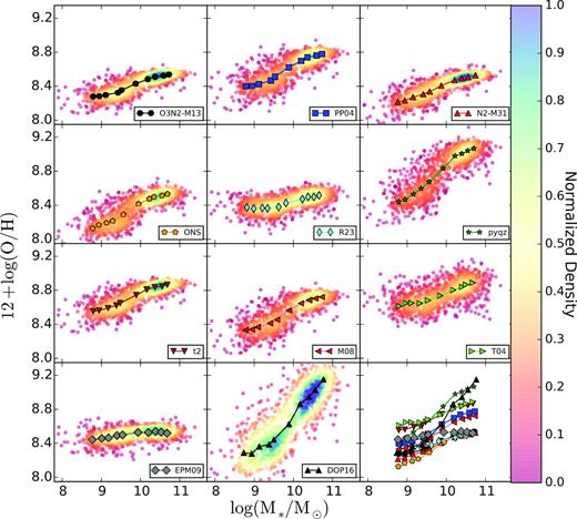
Mass–metallicity relation for the set of 11 oxygen abundance calibrators used in the present study for the sample of 1044 galaxies extracted from the SAMI galaxy survey. Each calibrator is shown in an individual panel, with the adopted name for the calibrator written in the corresponding inset. The coloured solid circles in each panel indicate the individual values of the stellar mass and oxygen abundance at the effective radius, colour-coded by the density of points (with blue meaning more dense areas, and red less dense ones). The single-colour symbols connected with a solid-black line represent the median value of the considered parameters at a set of bins described in the text. For comparison purposes, the median values for all the considered calibrators are included in the bottom-right panel. The different calibrators are described in the text.
It is clear that the absolute scale of the MZR depends on the adopted calibrator, as already described in many previous studies (e.g. Kewley & Ellison 2008; López-Sánchez et al. 2012; Barrera-Ballesteros et al. 2017; Sánchez et al. 2017). In general, calibrators based on the DM cover a smaller range of abundances (thus, smaller scatter) and lower values of the abundance on average than those based on photoionization models. Finally, mixed calibrators lie in between both of them. Indeed, as already noticed by Sánchez et al. (2017) and Barrera-Ballesteros et al. (2017), the dispersions around the average value in each mass bin are significantly larger for photoionization-model based calibrators, making them less suitable to explore possible secondary relations with other parameters if this dispersion is intrinsic to the calibrator itself. Finally, the t2 correction (Peimbert 1967) modifies the abundances based on the DM, increasing their values such that they are similar to those from photoionization models. This does not imply that the t2 makes the two abundances compatible. Some authors have suggested that a non-thermalized distribution of electrons in the nebulae, a physical process that produces similar results as a t2 distribution, could make both derivations of the oxygen abundance compatible (e.g. Nicholls, Dopita & Sutherland 2012; Nicholls et al. 2013; Dopita et al. 2013). This was refuted recently by Ferland et al. (2016). We consider that the nature of the t2 correction is different than the reason why the abundances based on the direct method and those based on photoionization models disagree (following Morisset et al. 2016). Therefore, from our point of view, it is a pure numerical coincidence that both abundances agree.
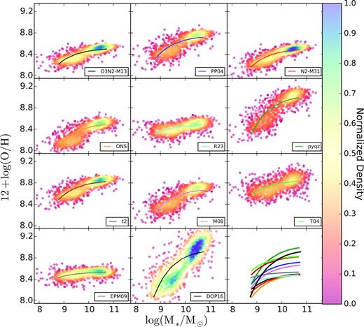
Best-fit MZR model for the different analysed calibrators. The coloured solid circles, in each panel, correspond to the values derived using each abundance estimator. Colours indicate the density of points. The solid lines with different colours represent the best-fit models, with each colour corresponding to one of the considered abundance calibrators. The best-fit models for all calibrators are shown in the bottom-right panel for comparison purposes.
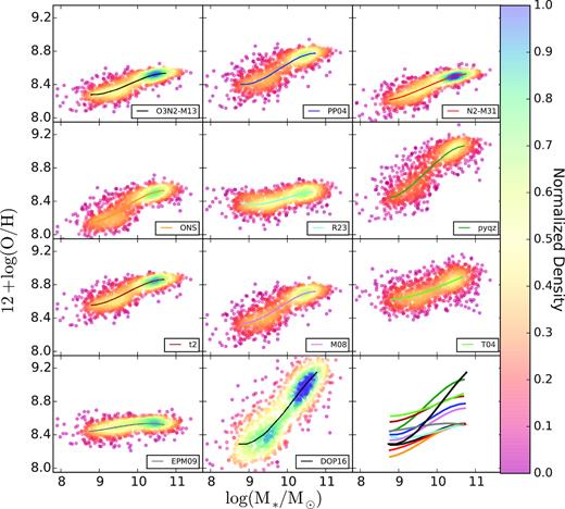
Best-fit pMZR model for the different analysed calibrators. The coloured solid circles, in each panel, correspond to the values derived using each abundance estimator. Colours indicate the density of points. The solid lines with different colours represent the best-fit models, with each colour corresponding to one of the considered abundance calibrators. The best-fit models for all calibrators are shown in the bottom-right panel for comparison purposes.
4.2 Dependence of the residuals of the MZR on SFR
We explore any possible secondary dependence of the MZR on SFR studying the correlations of the residuals of the two different characterizations of the MZ-distribution with this parameter. Then, we explore if introducing this dependence reduces the scatter in a significant way. Our reasoning is that any possible secondary relation that does not decrease significantly the scatter is not needed to describe the observed distributions.
In Fig. 4, we show the residuals of the oxygen for each calibrator as a function of the SFR, once subtracted the best-fitted MZR relation (Δlog (O/HMZR), left-hand panel) and pMZR relation (Δlog (O/HpMZR), right-hand panel). In both panels, we present the median values in SFR bins of 0.3 |$\log (\mathrm{M}_{\odot } \, \mathrm{yr^{-1}})$| width covering a range between –1.7 and 0.9 |$\log (\mathrm{M}_{\odot } \, \mathrm{yr^{-1}})$|. These bins were selected to include more than 20 objects in each bin, to guarantee robust statistics.
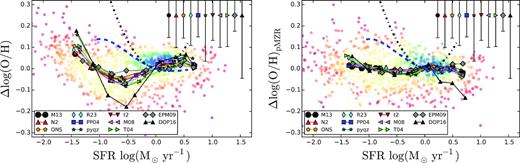
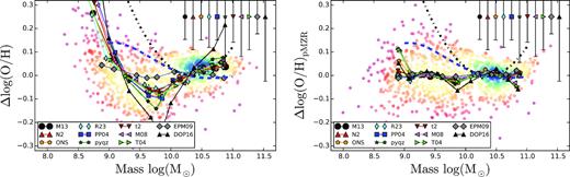
Residuals of the MZR (left-hand panel) and the pMZR (right-hand panel) from the different analysed calibrators against the SFR. For the cloud of data points we show the values estimated by the PP04 abundance calibrator, for simplicity. Each solid circle corresponds to an individual galaxy, colour-coded by density of points. The solid-lines, connecting different symbols, represent the median values in each SFR bin with each colour and symbol corresponding to a different calibrator, following the nomenclature shown in Fig. 1. The average standard deviation of the residuals for each calibrator is represented by an error bar at the top-right of each panel. In both panels, we show the expected residuals as a function of the SFR based on the relations proposed by Mannucci et al. (2010) (blue-dashed line), and by Lara-López et al. (2010) (black-solid line).
There is considerable agreement in the median of the residuals for most of the calibrators over the considered range of SFR. The one that deviates most is the DOP16. Despite these differences, the distribution of residuals is compatible with zero for all calibrators, taking into account the standard deviation of each individual bin (σ). In the case of the pMZR-residuals, the mean values are also compatible with zero, considering the error of the mean (i.e. σ/|$\sqrt{n}$|). The largest differences are found for the regime of lower SFRs (log SFR < −0.5). However, the different does not seem to be significant in an statistical way. For those galaxies that lie on the star-formation main sequence (SFMS), this SFR corresponds to stellar masses lower or of the order of 109.5 M⊙ (e.g. Cano-Díaz et al. 2016). In this regime we found a possible plateau in the MZ distribution (Fig. 1). Curiously, the trend described for the MZR-residual is different than the one found for the pMZR. In the previous one, galaxies with SFR between 0.1–0.4 M⊙yr−1 present a slightly lower oxygen abundance, contrary to the reported trends in the literature (e.g. Mannucci et al. 2010), rising again for SFRs lower than 0.05 M|$_\odot \, \rm yr^{-1}$| . For the pMZR residuals, the possible dependence with the SFR is even weaker, with a slight trend to higher abundances in the low SFR regime (log SFR < −1.5), but compatible with no dependence at any SFR.
Mannucci et al. (2010) and Lara-López et al. (2010) presented two different functional forms to describe the secondary relation that they found with the SFR. Both relations are quite different. The so called FMR relation (Mannucci et al. 2010) proposes a correction to the stellar-mass as independent parameter in the MZ-relation. On the other hand, the relation described by Lara-López et al. (2010), considers that the three parameters are located in a plane in the Mass-Metallicity-SFR space (the so-called MZ-SFR Fundamental-Plane). We compare with their predictions adopting the following procedure: (i) following Mannucci et al. (2010), we derive the average residual curve subtracting the MZR relation published by them, using their functional form and parameters, without a SFR dependence (i.e. μ0 of their equation 4) to the same relation, including this dependency (i.e. μ0.32 of their equation 4). When doing so, we assume that the SFR follows the stellar mass in a strict SFMS relation (by adopting the one published in Cano-Díaz et al. 2016). For this reason, this is just an average trend, and not the exact prediction of the FMR, that we will explore in following sections. The validity of the proposed average trend to describe the distribution of galaxies analysed by Mannucci et al. (2010) is discussed in detail in Appendix D. This average trend is shown as a dashed-blue line in Fig. 4. If the secondary relation found by Mannucci et al. (2010) was present for the average propulation of star-forming galaxies, this population should follow this dashed-blue line. However, if the driver for the FMR was the presence of a particular process in a particular group of galaxies (e.g. outflows present in extreme star-forming galaxies), the average population is not required to follow it. Therefore, we should clarify that the fact that they do not match with the data is not a definitive proof or disproof of the FMR, but a clue for its driver; (ii) For the MZ-SFR Fundamental Plane proposed by Lara-López et al. (2010) we just subtract the MZR estimated by them from their proposed FP (equation 1 of that article). In this case there is no assumption on the relation between the SFR and the stellar mass, and therefore, the prediction is exact, not a first order approximation, like the previous one. This trend is shown as a black-dotted line in Fig. 1. By construction the (Δlog (O/H) predicted by both relations is zero when the |$\log (\rm SFR/\mathrm{M}_{\odot } \, \mathrm{yr^{-1}}) = 0$|. In both cases the effect of introducing a secondary relation is more evident at low SFRs, that corresponds to lower regime of stellar masses (fig. 1 of Mannucci et al. 2010). A visual inspection of both figures shows that we cannot reproduce the predicted trends for any of the proposed relations, neither adopting the residuals of the MZR nor the pMZR ones. We should keep in mind that the disagreement is larger with the FP-relation suggested by Lara-López et al. (2010), for which we have not done any approximation. If the effects of the FMR are due to the residuals of the SFR with respect to the SFMS, there is still a possibility that our data are compatible with the proposed relation. We thus insist at this point, that this section is not a disproof of the FMR, but evidence that it is not driven by the main population of star-forming galaxies.
Based on a visual inspection we find no clear trend between the residuals of the two analysed functional forms of the MZ relation and the SFR. Nevertheless, we attempt to quantify whether a potential secondary relation may reduce the scatter around the mean distributions by performing a linear regression between the two parameters. The outcome of this analysis is included in Table 2, including the Pearson correlation coefficient, the best-fit parameters (slope and zero-point), and the standard deviation once the fitted linear relation was removed (ΔMZ-res), for both residuals, Δlog (O/HMZR) and Δlog (O/HpMZR), shown in Fig. 4. The correlation coefficients show that there is a very weak negative trend between the first residual and the SFR (rc ∼ −0.2), whose strength depends slightly on the calibrator, ranging from ∼−0.15 to ∼−0.25 for the EPM09 and pyqz calibrators respectively. For the second residual, there is an even weaker trend on average, with correlation coefficients ranging between ∼−0.05 and ∼−0.23 for the EPM09 and the DOP16 calibrators respectively. In agreement with the very low correlation coefficients, the derived zero-points of the relation are very near to zero for all considered calibrators, and statistically compatible with zero in many of them. Finally, the scatter of the residuals when considering a secondary dependence with the SFR, quantified by the standard deviation around the best-fit linear regression, is not improved for any of the analysed calibrators and adopted functional forms. In other words, the inclusion of this secondary relation does not provide a better representation of the data. Similar results were found by all similar analyses performed using up-to-date IFS data (e.g Sánchez et al. 2013, 2017; Barrera-Ballesteros et al. 2017).
Results of the linear fit of the residuals versus SFR for the two characterizations of the MZ-relation described in Section 4.1, MZR and pMZR. For the different metallicity calibrators we include the Pearson correlation coefficients between the two parameters (rc), together with the zero-points (α) and slopes (β) of the proposed linear relation, and the standard deviation around the best-fit regression (σ).
| Metallicity | ΔMZR versus SFR | ΔpMZR versus SFR | ||||||
|---|---|---|---|---|---|---|---|---|
| Indicator | rc | α | β | σ | rc | α | β | σ |
| O3N2-M13 | −0.22 | 0.008 ± 0.010 | 0.012 ± 0.013 | 0.105 | −0.10 | −0.007 ± 0.005 | −0.011 ± 0.007 | 0.077 |
| PP04 | −0.22 | 0.012 ± 0.015 | 0.019 ± 0.019 | 0.151 | −0.09 | −0.010 ± 0.007 | −0.016 ± 0.010 | 0.112 |
| N2-M13 | −0.22 | 0.009 ± 0.008 | 0.012 ± 0.011 | 0.107 | −0.17 | −0.006 ± 0.003 | −0.015 ± 0.005 | 0.077 |
| ONS | −0.22 | 0.007 ± 0.010 | 0.018 ± 0.016 | 0.142 | −0.13 | −0.007 ± 0.006 | −0.013 ± 0.010 | 0.100 |
| R23 | −0.20 | 0.006 ± 0.013 | 0.003 ± 0.017 | 0.101 | −0.08 | −0.008 ± 0.006 | −0.012 ± 0.008 | 0.087 |
| pyqz | −0.25 | 0.024 ± 0.020 | 0.021 ± 0.029 | 0.215 | −0.17 | −0.008 ± 0.006 | −0.010 ± 0.008 | 0.142 |
| t2 | −0.24 | 0.007 ± 0.012 | 0.012 ± 0.016 | 0.117 | −0.12 | −0.011 ± 0.006 | −0.015 ± 0.009 | 0.086 |
| M08 | −0.14 | 0.013 ± 0.015 | 0.023 ± 0.021 | 0.172 | −0.16 | −0.014 ± 0.007 | −0.019 ± 0.009 | 0.145 |
| T04 | −0.21 | 0.001 ± 0.021 | 0.002 ± 0.025 | 0.147 | −0.21 | −0.019 ± 0.007 | −0.026 ± 0.009 | 0.120 |
| EPM09 | −0.15 | 0.005 ± 0.005 | 0.005 ± 0.007 | 0.075 | −0.04 | 0.011 ± 0.006 | 0.010 ± 0.008 | 0.072 |
| DP09 | −0.17 | 0.010 ± 0.033 | 0.040 ± 0.043 | 0.295 | −0.23 | −0.066 ± 0.013 | −0.087 ± 0.018 | 0.202 |
4.3 Dependence of the residuals of the MZR on stellar mass
Mannucci et al. (2010) suggested that the secondary relation could be driven by galaxies of low-mass and large sSFR, and not only or mostly by the main population of star-forming galaxies. Similar results were presented by Amorín, Pérez-Montero & Vílchez (2010) and Telford et al. (2016). For this reason, it is important to explore the residuals of the MZR relation versus stellar mass. Fig. 5 shows the residuals of the oxygen abundance data after subtraction of the MZR and pMZR relations (i.e. the same values as shown in Fig. 4), but this time as a function of stellar mass. In both panels we present the median values in stellar-mass bins of 0.3 log (M⊙) width covering a range between 108 and 1011 M⊙. Like in the case of the analysis of the residuals as a function of the SFRs, we quantified the possible additional relation with the stellar mass by exploring the Pearson correlation coefficient, performing a linear regression between the two parameters, and deriving the standand deviations after removal of the best-fit linear regression. The results of this analysis are included in Table 3.
Residuals of the MZR (left-hand panel) and the pMZR (right-rpanel) for the different analysed calibrators against the stellar mass. For the data, we show the values estimated by the PP04 abundance calibrator, for simplicity. Each solid circle corresponds an individual galaxy, colour-coded by density of points. The solid lines, connecting different symbols, represent the median values in each SFR bin with each colour and symbol corresponding to a different calibrator, following the nomenclature shown in Fig. 4. The average standard-deviation of the residuals for each calibrator is represented by an error bar at the top-right of each panel. In both panels, we show the expected residuals as a function of the SFR based on the relations proposed by Mannucci et al. (2010) (blue-dashed line), and by Lara-López et al. (2010) (black-solid line).
Results of the linear fit of the residuals of the two characterizations of the MZ-relation described in Section 4.1, MZR and pMZR, versus the stellar mass. For the different metallicity calibrators, we include the Pearson correlation coefficients between the two parameters (rc), together with the zero-points (α) and slopes (β) of the proposed linear relation, and the standard deviation around the best-fit regression (σ).
| Metallicity | ΔMZR versus Mass | ΔpMZR versus Mass | ||||||
|---|---|---|---|---|---|---|---|---|
| Indicator | rc | α | β | σ | rc | α | β | σ |
| O3N2-M13 | −0.06 | 0.253 ± 0.359 | −0.023 ± 0.036 | 0.097 | 0.07 | −0.050 ± 0.037 | 0.005 ± 0.004 | 0.077 |
| PP04 | −0.06 | 0.345 ± 0.513 | −0.031 ± 0.051 | 0.140 | 0.07 | −0.074 ± 0.054 | 0.007 ± 0.005 | 0.111 |
| N2-M13 | −0.02 | 0.184 ± 0.350 | −0.016 ± 0.035 | 0.099 | 0.02 | 0.019 ± 0.044 | −0.002 ± 0.004 | 0.078 |
| ONS | −0.10 | 0.498 ± 0.481 | −0.046 ± 0.048 | 0.130 | −0.01 | 0.065 ± 0.104 | −0.006 ± 0.010 | 0.101 |
| R23 | −0.05 | 0.452 ± 0.386 | −0.044 ± 0.039 | 0.099 | 0.06 | −0.057 ± 0.050 | 0.006 ± 0.005 | 0.087 |
| pyqz | −0.11 | 0.622 ± 0.764 | −0.057 ± 0.077 | 0.194 | −0.06 | 0.168 ± 0.127 | −0.016 ± 0.013 | 0.142 |
| t2 | −0.08 | 0.287 ± 0.405 | −0.026 ± 0.040 | 0.109 | 0.05 | −0.029 ± 0.066 | 0.003 ± 0.007 | 0.086 |
| M08 | 0.02 | −0.058 ± 0.443 | 0.008 ± 0.044 | 0.170 | −0.02 | 0.173 ± 0.152 | −0.017 ± 0.015 | 0.145 |
| T04 | −0.03 | 0.481 ± 0.504 | −0.048 ± 0.052 | 0.141 | −0.09 | 0.334 ± 0.180 | −0.034 ± 0.019 | 0.121 |
| EPM09 | −0.08 | 0.126 ± 0.078 | −0.012 ± 0.008 | 0.073 | 0.07 | −0.082 ± 0.040 | 0.009 ± 0.004 | 0.072 |
| DP09 | 0.06 | 0.430 ± 1.163 | −0.038 ± 0.119 | 0.275 | −0.08 | 0.228 ± 0.169 | −0.024 ± 0.017 | 0.201 |
If the adopted functional form for the MZ relation was representative of the distribution, there should not be any significant additional correlation with the stellar mass of the residuals of that relation. Indeed, the correlation coefficients between the residuals and the stellar mass are very low, of the order of ±0.1, and the slopes of the derived linear regressions are in general consistent with zero. The introduction of an additional dependence with the mass does not decrease the scatter of the residuals neither. Like in the case of the distribution of residuals against the SFR, the largest differences are found for the MZR relation, in the low-Mass regime. Indeed, even for the pMZR relation, the scatter seems to increase slightly at lower stellar masses, where we found the larger number of outliers. Thus, it is still possible that the trends described by Mannucci et al. (2010) can only be found for low-mass galaxies.
4.4 Studying the FMR in detail
We have shown that the residuals of the MZR and pMZR relations do not show a clear dependence on the SFR for any of the analysed calibrators, and only a possible weak trend for low stellar masses. As indicated before, we used the assumption of a linear trend with SFR for this exploration. Therefore, strictly speaking, our results do not agree with a hypothetical linear secondary relation with the SFR, i.e. the relation proposed by Lara-López et al. (2010).
The distribution of the oxygen abundances over the μ* parameter for the different calibrators is shown in Fig. 6 (following the same nomenclature as in Fig. 1). The shape of the different distributions for each calibrator is very similar, with the same pattern already described in Section 4.1. Like the Mass–Metallicity relation, we characterize the μ*–Metallicity relation using the same parameterization as described in equations (1) and (2), substituting the stellar mass by μ*. We will refer them as the FMR and pFMR, respectively. Table 5 lists the best-fit parameters for both functional forms adopted to characterize the shape of the relation between μ* and the oxygen abundance, together with the corresponding standard deviations around the best-fit curves.

In the case of the FMR parameterization, the values for the asymptotic oxygen abundance (a) are very similar, irrespectively of whether we use M* or μ*. The parameter that defines the strength of the bend of the distribution, b is of the same order for both distributions. For the pFMR parameterization, the coefficients are more difficult to interpret, although in general they are of the same order as those found for the pMZR. Finally, we do not find any significant decrease in the standard deviation of the distribution of the oxygen abundance residuals when introducing the proposed secondary dependence on the SFR, as can be verified by comparing the values in Table 4 with the corresponding ones in Table 1.
Best-fit parameters for the two functional forms adopted to characterize the FMR and their scatter for the different abundance estimations considered in our analysis. We include, for each different calibrator, (i) the standard deviation of the values of the oxygen abundance (σlog(O/H)); (ii) the best-fit a and b parameters as described in equation (1), applied to the FMR (i.e. modifying the mass by the μ*, 0.32 parameter); (iii) the standard deviation of the abundances once subtracted the best-fit curve, characterized by equation (1) and the parameters indicated before (σFMR); (iv) the coefficients of the polynomial function adopted in equation (2), defined as the pFMR relation (i.e. modifying the mass by the μ*, 32 parameter) and finally, (v) the standard deviation once subtracted the best-fit polynomial function, σpFMR. The values of the different parameters are shown up to the third decimal to highlight the differences. However, we consider that only the first two decimals are significant.
| Metallicity | FMR Best Fit | σFMR | pFMR Polynomial fit | σpFMR | ||||
|---|---|---|---|---|---|---|---|---|
| Indicator | a | b | (dex) | p0 | p1 | p2 | p3 | (dex) |
| O3N2-M13 | 8.55 ± 0.01 | 0.016 ± 0.002 | 0.086 | 8.219 ± 0.236 | −0.392 ± 0.372 | 0.421 ± 0.188 | −0.086 ± 0.031 | 0.071 |
| PP04 | 8.80 ± 0.02 | 0.024 ± 0.002 | 0.125 | 8.268 ± 0.356 | −0.503 ± 0.556 | 0.582 ± 0.279 | −0.121 ± 0.045 | 0.103 |
| N2-M13 | 8.54 ± 0.01 | 0.017 ± 0.001 | 0.085 | 7.681 ± 0.155 | 0.306 ± 0.252 | 0.112 ± 0.130 | −0.041 ± 0.022 | 0.075 |
| ONS | 8.56 ± 0.02 | 0.022 ± 0.002 | 0.117 | 9.179 ± 0.482 | −2.244 ± 0.754 | 1.444 ± 0.377 | −0.260 ± 0.061 | 0.102 |
| R23 | 8.51 ± 0.03 | 0.007 ± 0.003 | 0.090 | 10.996 ± 0.961 | −4.270 ± 1.498 | 2.218 ± 0.756 | −0.362 ± 0.124 | 0.114 |
| pyqz | 9.08 ± 0.04 | 0.032 ± 0.003 | 0.167 | 9.241 ± 0.344 | −2.262 ± 0.567 | 1.653 ± 0.298 | −0.312 ± 0.051 | 0.140 |
| t2 | 8.89 ± 0.02 | 0.018 ± 0.001 | 0.094 | 8.358 ± 0.180 | −0.267 ± 0.286 | 0.408 ± 0.145 | −0.088 ± 0.024 | 0.080 |
| M08 | 8.97 ± 0.01 | 0.026 ± 0.001 | 0.153 | 7.961 ± 0.293 | 0.115 ± 0.458 | 0.301 ± 0.229 | −0.077 ± 0.037 | 0.139 |
| T04 | 8.88 ± 0.04 | 0.012 ± 0.003 | 0.130 | 11.572 ± 1.122 | −4.755 ± 1.748 | 2.449 ± 0.880 | −0.390 ± 0.144 | 0.143 |
| EPM09 | 8.55 ± 0.01 | 0.007 ± 0.001 | 0.073 | 7.750 ± 0.267 | 0.767 ± 0.450 | -0.217 ± 0.240 | 0.014 ± 0.041 | 0.073 |
| D0P09 | 9.12 ± 0.06 | 0.047 ± 0.005 | 0.254 | 9.050 ± 0.239 | −2.226 ± 0.377 | 1.549 ± 0.190 | −0.264 ± 0.031 | 0.188 |
Parameters derived for the generalized FMRd relation derived by the adopted fitting process, when the d parameter in equation (4) is not fixed to the value reported in the literature. We report the three parameters included in equation (3) (a, b and d), together with the standard deviation of the oxygen abundances after subtraction of the best-fit FMRd relation (σ MZ-res). The best-fit d parameter derived when adopting a polynomial functional form for the FMR (pFRMd formalism), is reported too. In this particular case, we adopted equation (3), substituting the stellar mass by the μ*, d parameter. Finally, we list the standard deviations after subtraction of the best-fit pFRMd model. All these parameters are included for the different estimations of oxygen abundance included in this study. Like in the previous tables some parameters are presented including the third decimal, to highlight the differences, although we consider that the values are significant only to the second decimal.
| Metallicity | Generalized FMR Best Fit | σd FMR-res | pFMR best fit | σd pFMR-res | ||
|---|---|---|---|---|---|---|
| Indicator | a (dex) | b (dex /log (M⊙)) | d (dex|$/\log (\mathrm{M}_{\odot }\, \mathrm{yr}^{-1})$| | (dex) | d (dex|$/\log (\mathrm{M}_{\odot }\, \mathrm{yr}^{-1})$| | (dex) |
| O3N2-M13 | 8.55 ± 0.02 | 0.020 ± 0.003 | −0.498 ± 0.054 | 0.077 | −0.395 ± 0.063 | 0.069 |
| PP04 | 8.80 ± 0.02 | 0.029 ± 0.004 | −0.498 ± 0.045 | 0.111 | −0.395 ± 0.052 | 0.100 |
| N2 | 8.54 ± 0.02 | 0.021 ± 0.003 | −0.470 ± 0.050 | 0.079 | −0.388 ± 0.059 | 0.071 |
| ONS | 8.54 ± 0.02 | 0.022 ± 0.004 | −0.421 ± 0.058 | 0.110 | −0.285 ± 0.076 | 0.097 |
| R23 | 8.54 ± 0.02 | 0.017 ± 0.003 | −0.631 ± 0.065 | 0.083 | −0.541 ± 0.071 | 0.081 |
| pyqz | 9.06 ± 0.03 | 0.034 ± 0.004 | −0.419 ± 0.045 | 0.160 | −0.277 ± 0.057 | 0.136 |
| t2 | 8.88 ± 0.02 | 0.022 ± 0.003 | −0.479 ± 0.050 | 0.086 | −0.389 ± 0.059 | 0.078 |
| M08 | 8.98 ± 0.02 | 0.034 ± 0.004 | −0.511 ± 0.044 | 0.141 | −0.448 ± 0.048 | 0.135 |
| T04 | 8.89 ± 0.02 | 0.022 ± 0.004 | −0.577 ± 0.062 | 0.124 | −0.429 ± 0.078 | 0.117 |
| EPM09 | 8.56 ± 0.02 | 0.008 ± 0.003 | −0.548 ± 0.122 | 0.069 | −0.602 ± 0.085 | 0.067 |
| DP09 | 9.08 ± 0.03 | 0.057 ± 0.005 | −0.502 ± 0.032 | 0.226 | −0.375 ± 0.039 | 0.185 |
So far, we do not find a decrease in the global standard deviation in the same way as the one reported by Mannucci et al. (2010), neither using and fitting for the proposed parameterization for the dependence on SFR nor directly using the reported values for the proposed correction. Therefore, we cannot confirm their results with the current analysis and data set in this respect. However, it is still possible that there is no global improvement in the scatter over the total range of masses and star formation rates but the introduction of a secondary relation could improve the representation of the data in certain mass or star-formation ranges. In this regard previous results (e.g. Sánchez et al. 2017) were not totally conclusive. For some calibrators it seems that the dispersion decreases when introducing the secondary relation at low masses (M* < 109.5M⊙). In order to perform this test we split the data set in different ranges of stellar masses and star-formation rates and compared the mean value and the standard deviations of both the best-fit FMRd and MZR for each considered data set.
The result of this analysis is illustrated by Fig. 7, where we show the distribution for one particular calibrator (t2). The same qualitative results are derived using any of the considered calibrators, but we describe in detail the results for only one just for clarity. The figure shows the individual t2 oxygen abundances for each galaxy as a function of stellar mass, separated in five SFR bins. Following Mannucci et al. (2010) and Andrews & Martini (2013), in addition we represent the average FMRd relation derived for each bin, and the derived MZR (Table 1). Thus, the relation assuming d = 0. A visual inspection of the Figure gives the impression that when including an additional dependence with the SFR, with the functional form presented in Mannucci et al. (2010), a better description of the data is obtained. This is even more clear for the mean values in bins of stellar masses, derived using the same scheme adopted in Fig. 1 and Section 4.1, shown as solid squares in Fig. 7.
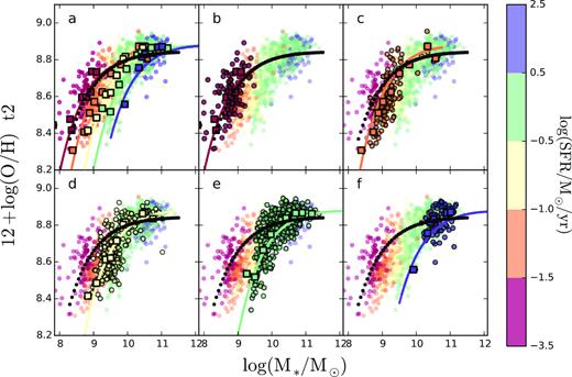
Mass–metallicity relations using the oxygen abundances derived using the t2 calibrator for the sample of galaxies analysed in this study. Solid circles represent the values for each single galaxy, colou-coded by the SFR as indicated by the colourbar. The solid squares represent the average values in the same stellar mass bins as shown in Fig. 1. Panel (a) includes the full data set, together with the average μ*, dZ relations derived for each SFR bin. These models correspond to the parameterization described in equation (4), using the values listed in Table 5. The black dotted line corresponds to the original MZ relation, not considering the possible relation with the SFR, i.e. to the parameterization described in equation (1), using the values reported in Table 1. Each individual panel from (b) to (f) corresponds to a different SFR bin, ranging from the lowest to the highest values of the star-formation rate.
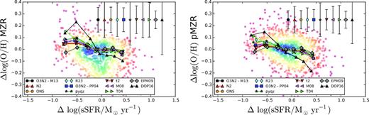
Distribution of the residuals of the oxygen abundance after removal of the dependence with the stellar mass (the MZR), as a function of the residuals of the sSFR after removal of the dependence on stellar mass (the SFMS). Solid circles represent the individual values when adopting the PP04 calibrator (colour codded by the density of points), and the line-connected symbols represent the median value of the oxygen abundance residuals as a function of the median value of the sSFR in a set of bins (in this later parameter). The symbols are the same as the ones adopted in Fig. 4.
However, when comparing the differences between the global MZR and the FMRd in different SFR ranges, at the range of stellar masses sampled by the corresponding points, it is evident that the differences in the representation of the full population of galaxies are not large. Table 6 shows a detailed comparison of the different residuals after subtraction of the derived FMRd, MZR and pMZR relations, described in the previous sections. In general, the residuals around the FMRd relation are more consistent with zero, with slightly lower scatter, than those of the MZR. However, contrary to what is predicted by the proposed FMR, the residuals of the MZR do not present a systematic trend with larger abundances for lower SFRs and smaller abundances for higher SFRs. For example, for very low SFRs (|$\lt 10^{-1.5} \, \mathrm{M}_\odot \, \mathrm{yr}^{-1}$|) there is a positive deviation in the residual of ∼0.04 ± 0.14 dex, however, for SFRs between 10|$^{-1.5}-10^{-1} \, \mathrm{M}_\odot \, \mathrm{yr}^{-1}$|, the deviation is negative (∼−0.05 ± 0.09 dex: i.e. contrary to that proposed by the FMR picture). On the other hand, for the explored ranges in the stellar mass there is no general improvement in the residuals, being appreciable only for stellar masses below 10|$^{9.5} \, \mathrm{M}_\odot$|. Even more, both residuals show a rather similar and consistent trend to mis-represent the data at low masses. This is consistent with a polynomial function representing the data better than the assumed functional form. Indeed, in these mass regime the residuals of the pMZR are smaller than those of the FMRd. For the pMZR the introduction of a secondary dependence with the SFR only slightly reduces the scatter in the residuals for the more massive galaxies. Thus, the trend with the SFR is different if we represent the MZ distribution using two different functional forms.
Comparison of the residuals from the FMRd and MZR relations, based on the adopted fitting procedure (i.e. using the values listed in Tables 5 and 1), in five bins of SFRs and stellar masses, respectively. We list (i) the SFRs and stellar masses covered, (ii) the mean SFR (<SFR>), with its standard deviation, and finally (iii) the mean values and standard deviations of the residuals for the two relations explored here. We include the third decimal in the parameters to highlight the differences. However, we remind the reader that we do not consider significant those values beyond the second decimal.
| |$\log (\rm SFR/\mathrm{M}_\odot \, \mathrm{yr}^{-1})$| | <log (SFR)> | FMRd-res | MZR-res | pMZR-res |
|---|---|---|---|---|
| range | |$\log(\, \mathrm{M}_\odot \, \mathrm{yr}^{-1})$| | (dex) | (dex) | (dex) |
| [-3.5,-1.5] | −1.80 ± 0.27 | −0.001 ± 0.113 | 0.038 ± 0.135 | 0.023 ± 0.124 |
| [-1.5,-1] | −1.23 ± 0.15 | −0.043 ± 0.082 | −0.075 ± 0.090 | 0.004 ± 0.098 |
| [-1,-0.5] | −0.74 ± 0.15 | −0.042 ± 0.085 | −0.086 ± 0.098 | −0.013 ± 0.084 |
| [-0.5,0.5] | −0.01 ± 0.28 | 0.018 ± 0.072 | −0.022 ± 0.091 | −0.012 ± 0.073 |
| [0.5,2.5] | 0.75 ± 0.17 | 0.042 ± 0.062 | −0.001 ± 0.068 | −0.022 ± 0.067 |
| log (M*/M⊙) | <log (SFR)> | FMRd-res | MZR-res | pMZR-res |
|---|---|---|---|---|
| range | |$\log(\, \mathrm{M}_\odot \, \mathrm{yr}^{-1})$| | (dex) | (dex) | |
| [8,9.5] | −1.26 ± 0.45 | −0.040 ± 0.088 | −0.068 ± 0.115 | −0.001 ± 0.102 |
| [9.5,10] | −0.42 ± 0.33 | −0.023 ± 0.097 | −0.084 ± 0.104 | −0.015 ± 0.101 |
| [10,10.5] | 0.01 ± 0.42 | 0.036 ± 0.056 | 0.004 ± 0.056 | −0.002 ± 0.055 |
| [10.5,11] | 0.28 ± 0.44 | 0.030 ± 0.050 | 0.018 ± 0.050 | −0.011 ± 0.051 |
| [11,12.5] | 0.30 ± 0.52 | −0.002 ± 0.068 | 0.010 ± 0.066 | 0.024 ± 0.074 |
Finally, the standard deviation of the distribution of the residuals indicates that there is no significant improvement for all the explored ranges of SFRs and stellar masses. For the MZR the reduction ranges between 0.008 and 0.022 dex for the SFR bins and between 0.000 and 0.027 dex for the stellar mass ones, although, in general, the reduction is of the order of 0.01 dex. On the other hand, for the pMZR the reduction of the scatter, if any, is at the third decimal of the standard deviation. In summary, if there is an improvement by introducing a secondary relation with the SFR (a) it seems to be limited to some particular ranges of SFRs or stellar masses, and (b) its quantitative effect depends on the adopted parameterization of the MZ-relation and the adopted calibrator. In general, the data points are well described with the pMZR model, without assuming any secondary dependence on SFR.
4.5 Exploring in detail the Mass-SFR-Z plane
Contrary to previous proposed relations between the stellar mass and the oxygen abundance, these authors propose that the relation between both parameters is linear, departing from the usual shape shown before. In Section 4.2 we have already shown that we cannot reproduce the observed distribution of the residuals of the MZR and pMZR with the relation proposed by Lara-López et al. (2010) (Fig. 4), and that imposing a linear relation of those residuals with the SFR does not improve its scatter. However, since we have adopted a different calibrator for the oxygen abundance and we use a significantly different sample, maybe the actual parameters for the proposed functional form could be different. Therefore, we have fitted equation (5) to our data set to provide the best representation of the data considering the functional form suggested by Lara-López et al. (2010).
Table 7 shows the result of this analysis, including the best-fit parameters for each calibrator together with the standard deviation of the residuals. The comparison of these standard deviations with the ones shown in Table 1, shows that in general the proposed functional form decreases the dispersion marginally for all calibrators when compared with the MZR. However, it does not provide any improvement with respect to the pMZR relation, that, as indicated before, does not include the SFR as a third parameter. Further, assuming just a linear dependence on stellar mass, the reported scatter of the residuals is very similar to the one reported here. In summary, we cannot reproduce the results found by Lara-López et al. (2010), assuming their proposed parameterization.
Parameters derived for the linear M-SFR-Z relation, when considering the functional form suggested by Lara-López et al. (2010) (equation 5), based on the described fitting procedure. We include the best-fit α, β and γ parameters of the equation for each different calibrator, together with the standard deviation after subtraction of the derived model (σ FP-res). As in previous tables, some values are represented to the third decimal to show any possible difference, although we consider that the values are significant only to the second decimal.
| Metallicity | FP Best Fit | σ FP-res | ||
|---|---|---|---|---|
| Indicator | α | β | γ | (dex) |
| O3N2 | 0.19 ± 0.02 | −0.054 ± 0.022 | 8.044 ± 0.054 | 0.074 |
| PP04 | 0.27 ± 0.03 | −0.078 ± 0.027 | 8.062 ± 0.065 | 0.106 |
| N2 | 0.21 ± 0.02 | −0.059 ± 0.022 | 7.972 ± 0.055 | 0.076 |
| ONS | 0.23 ± 0.03 | −0.041 ± 0.027 | 7.916 ± 0.066 | 0.102 |
| R23 | 0.13 ± 0.03 | −0.063 ± 0.024 | 8.155 ± 0.058 | 0.084 |
| pyqz | 0.35 ± 0.03 | −0.056 ± 0.031 | 8.117 ± 0.077 | 0.144 |
| t2 | 0.21 ± 0.03 | −0.057 ± 0.024 | 8.302 ± 0.058 | 0.083 |
| M08 | 0.31 ± 0.03 | −0.105 ± 0.031 | 8.123 ± 0.076 | 0.143 |
| T04 | 0.19 ± 0.03 | −0.078 ± 0.029 | 8.357 ± 0.070 | 0.121 |
| EPM09 | 0.06 ± 0.02 | −0.017 ± 0.022 | 8.391 ± 0.054 | 0.071 |
| DOP09 | 0.59 ± 0.04 | −0.200 ± 0.037 | 7.488 ± 0.089 | 0.194 |
4.6 The [O/H]-SFR relation after subtraction of the stellar mass dependences
This selection has a limited effect on the sample, that now comprises 1020 galaxies. Indeed, not making that selection does not change significantly the results, but we prefer to keep it as it was the procedure adopted in previous studies.
Then, we remove the dependence of the oxygen abundance on the stellar mass by adopting a similar procedure. However, in this case we have two possible parameterizations for this dependence, as discussed in Section 4.1, that we defined as MZR (equation 1) and pMZR (equation 2), using the residuals discussed in Section 4.2, defined as ΔMZR and ΔpMZR. Adopting this procedure, we totally remove the dependence of the two (oxygen abundances and SFRs) on stellar mass. We should note that selecting particular ranges of masses and looking for possible secondary dependences with the SFR does not guarantee that the primary dependence with the mass is totally removed. This procedure was adopted in previous sections and implemented in several previous studies (e.g. Salim et al. 2014). However, the selection of a range of parameters, even a narrow one, may retain part of the dependence with the stellar mass.
Fig. 8 shows the distribution of the two considered residual abundances, ΔMZR and ΔpMZR, over the residuals of the specific star-formation rate Δlog sSFR, for the different calibrators discussed in this article. The cloud of points corresponds to the distribution for the O3N2-PP04 calibrator, with the distribution of the remaining calibrators represented by the average value in a set of bins in Δlog sSFR of 0.3 dex width. We selected this calibrator just because it is at the average location of the remaining ones, due to its mixed nature (e.g. Sánchez et al. 2017), but beyond that it is irrelevant which calibrator is shown in the figure. For the ΔMZR most of the calibrators show no clear trend between both residuals, and there is only a very mild trend in the case of the ΔpMZR residuals. The calibrator for which the trend seems to be stronger is the DOP16 one, this particular trend being consistent with the predictions of the FMR.
We quantify the possible correlations between both parameters by (1) deriving the Pearson correlation coefficient (rc) between both parameters for each calibrator, and (2) by performing a linear regression and determining if the scatter is reduced with respect to the one observed in the original MZR distribution. The results of this analysis are listed in Table 8, including the rc coefficient together with the parameters of the linear fitting and the standard deviations of the residuals after subtraction of the best-fit model. The reported correlation coefficients indicate that across all the calibrators there is either a weak correlation (rc ∼ −0.35) or no correlation (rc ∼ −0.14) between the residuals. This result has a very high significance level, with a probability larger than 99.99 per cent in all the cases. Consistently, the slopes reported by the linear regression are very small, and there is little or no reduction of the scatter.
Results of the study of the possible relation between the residuals of the oxygen abundance and the sSFR after removal of the corresponding dependences on stellar mass (i.e. the MZ and SFMS relations), for the different estimations of the oxygen abundances shown in Fig. 8. We include the Pearson correlation coefficient between the two parameters (rc), the zero-point (α) and the slope (β) for the best-fit linear relation, and the standard deviation when this relation is subtracted (σ-res). We report the values for the residuals of both functional forms adopted for the mass–metallicity relation, the MZR and the pMZR parameterize.
| Metallicity | rc | Δlog O/H-MZR versus Δlog (sSFR) | σ-res | rc | Δlog O/H-pMZR versus Δlog (sSFR) | σ-res | ||
|---|---|---|---|---|---|---|---|---|
| Indicator | α (dex) | β (dex /log (yr−1)) | (dex) | α (dex) | β (dex /log (yr−1)) | (dex) | ||
| O3N2-M13 | −0.287 | 0.01 ± 0.01 | −0.06 ± 0.01 | 0.096 | −0.290 | −0.01 ± 0.01 | −0.06 ± 0.01 | 0.074 |
| PP04 | −0.286 | 0.01 ± 0.01 | −0.08 ± 0.01 | 0.139 | −0.288 | −0.02 ± 0.01 | −0.09 ± 0.02 | 0.108 |
| N2-M13 | −0.297 | 0.01 ± 0.01 | −0.05 ± 0.01 | 0.098 | −0.323 | −0.01 ± 0.01 | −0.05 ± 0.02 | 0.074 |
| ONS | −0.220 | 0.01 ± 0.01 | −0.05 ± 0.01 | 0.136 | −0.235 | −0.01 ± 0.01 | −0.06 ± 0.01 | 0.099 |
| R23 | −0.310 | −0.01 ± 0.01 | −0.10 ± 0.01 | 0.095 | −0.278 | −0.01 ± 0.01 | −0.11 ± 0.01 | 0.084 |
| pyqz | −0.224 | 0.02 ± 0.01 | −0.09 ± 0.01 | 0.206 | −0.237 | −0.01 ± 0.01 | −0.08 ± 0.01 | 0.138 |
| t2 | −0.289 | −0.01 ± 0.01 | −0.07 ± 0.01 | 0.108 | −0.299 | −0.01 ± 0.01 | −0.06 ± 0.01 | 0.082 |
| M08 | −0.287 | 0.01 ± 0.01 | −0.10 ± 0.01 | 0.141 | −0.300 | −0.02 ± 0.01 | −0.09 ± 0.02 | 0.108 |
| T04 | −0.263 | 0.01 ± 0.01 | −0.16 ± 0.03 | 0.141 | −0.248 | −0.02 ± 0.01 | −0.14 ± 0.01 | 0.119 |
| EPM09 | −0.136 | −0.01 ± 0.01 | 0.01 ± 0.02 | 0.073 | −0.142 | −0.01 ± 0.01 | −0.01 ± 0.02 | 0.070 |
| DOP09 | −0.316 | −0.01 ± 0.02 | −0.24 ± 0.05 | 0.273 | −0.348 | −0.06 ± 0.01 | −0.26 ± 0.03 | 0.194 |
In summary, our results do not show a clear secondary relation between the oxygen abundance and the SFR after removal of the dependence of both on stellar mass.
5 DISCUSSION
We explore the mass–metallicity relation based on the most recent data set provided by the SAMI survey comprising a total of 2273 of galaxies. For 1044 of those, we derive the stellar mass, the oxygen abundance, and the star formation rate. In the current analysis, we followed the procedures applied on previous IFU surveys, for a sample with a size between the one explored by Sánchez et al. (2017) for the CALIFA survey and the one explored by Barrera-Ballesteros et al. (2017) for the MaNGA survey. Adopting a set of different abundance calibrators we determine the shape of the MZ relation in the most general way, exploring the possible dependence with the star-formation rate. The previously reported trend of this relation described in many different publications (e.g. Tremonti et al. 2004) is confirmed. We found that this shape is described well, for most of the adopted calibrators, by a linear + exponential functional form like the one adopted by Sánchez et al. (2015) (MZR parameterization). However, it is much better described by a fourth-order polynomial function, similar to the one adopted by Kewley & Ellison (2008) (pMZR parameterization). The main difference between the different abundances calibrators is found in the asymptotic value found at the high-mass end, and in the scatter around the best-reported relations. The reported relation is as tight as the one usually reported for single-aperture spectroscopic surveys (∼0.1 dex Tremonti et al. 2004) for most of the adopted calibrators, but not as tight as the one found in previous IFU surveys (∼0.05 dex Sánchez et al. 2013, 2017; Barrera-Ballesteros et al. 2017). Those calibrators based on photoionization models present the larger scatter around the mean distribution over stellar mass, as already noticed by Sánchez et al. (2017), although the differences are much larger than in the case of previous IFU studies. The smaller field-of-view and somewhat more coarse spatial sampling of the SAMI data may introduce a larger uncertainty in the oxygen abundance derivation based on the radial profile when compared to the CALIFA ones. However, the spatial sampling in SAMI is better than in MaNGA, in general, and the FoV is similar for at least 1/3 of the sampled objects. Therefore, this should not be a major driver for potential differences. Indeed, the main trends remain very similar among the three data sets, as shown in Fig. C1.
We study the different scenarios proposed in the literature to describe a possible secondary relation of the oxygen abundance and the mass–metallicity relation with the SFR in the broadest possible way. We assume that the abundance depends primarily on stellar mass, and explored (i) if the residuals of the best-fit MZ relations adopting two different functional forms do indeed correlate with the SFR, (ii) how well the data are represented by so-called Fundamental Mass-Metallicity Relation proposed by (Mannucci et al. 2010), or a relation with a similar functional form and different fitted parameters, (iii) how well the data are represented by a functional form similar to the so-called Fundamental Plane of Mass-SFR-Z, proposed by Lara-López et al. (2010), and (iv) if there is a relation between the residuals of both the oxygen abundances and the SFRs once considered their respective dependence on stellar mass. In none of these cases did we find either a strong or moderate secondary correlation with the SFR or a clear improvement in the scatter when introducing this third parameter. This result is summarized in Fig. 9, where the standard deviation of the oxygen abundance around the mean value is shown together with the standard deviations of the residuals for each adopted functional form. We represent the mean value (central point) and the standard deviation (error bars) among the values reported for the eleven calibrators considered along this study. The figure illustrates clearly that there is no reduction in the scatter when by introducing any of the analysed secondary relations with the SFR neither for the MZR nor for the pMZR parameterizations. If there is any improvement, it is marginal, in particular if the MZR-parameterization is adopted, and for certain calibrators, and/or in some particular ranges of the analysed parameters. This is the case of the calibrators with the larger initial scatter, which may indicate that they present secondary trends with other parameters, like the ionization strength, somehow correlated with the SFR.
Average standard deviations of the distributions of oxygen abundances for each of the considered calibrators for (1) the original distribution of abundances, (2) the residuals from the best-fit MZR and pMZR parameterization, (3) the residuals from the linear regression of the residuals after subtraction of the best-fit MZR and pMZR models, (4) the residuals of the best-fit Fundamental Plane, (5) the residuals of the best-fit FMR and pFMR models, and (6) the residuals of the best linear regression of the analysis of the distribution of the oxygen abundance against the SFR after subtraction of the dependence on stellar mass. The error bars indicate the standard deviation around the mean values derived for each calibrator in each of the considered analysis. This figure summarizes the content of all the results in the present study.
Sánchez et al. (2017) reported a possible dependence with the SFR confined to the regime of low masses (M < 109.5 M⊙). We cannot confirm that result. We only find a mild improvement in this regime (∼0.02 dex in the mean value and ∼0.02 dex in the dispersion), when comparing a generalized FMR relation (allowing to vary the parameter that introduces the dependence with the SFR) with the MZR-parameterization. However, when introducing a polynomial function (the pMZR-parameterization), the improvement is mimimized (no improvement in the mean value and ∼0.02 dex in the dispersion). Since this latter functional form was not discussed in detail in this previous article we cannot determine if the nature of the difference is due to the use of this new parameterization of the relation between the oxygen abundance and the stellar mass. However, we can claim that if there is a secondary relation this would be confined to the low stellar mass regime.
In general, our results are consistent with those reported by previous IFU surveys (Sánchez et al. 2013, 2017; Barrera-Ballesteros et al. 2017). These results thus support the claim by Sánchez et al. (2013) that there is no need to introduce the SFR as a secondary parameter to describe the distribution of oxygen abundances. Other authors are not able to reproduce this secondary relation either (e.g. Kashino et al. 2016), or found a much weaker ones (e.g. Telford et al. 2016) in different data sets. The current analysis stresses the need for a good parameterization of the relation between oxygen abundance and its primarily tracer, the stellar mass. Being constrained to a particular functional form, like the MZR-parameterization, may lead to the wrong impression that there is a possible secondary dependence with the SFR for some particular calibrators (although the effect is not significant). The introduction of different functional forms, like the polynomial pMZR-parameterization blurs the effect of the SFR. This is particularly important since the dependence of the oxygen abundance on stellar mass is not linear, but the one between the SFR and the mass is. Indeed, in some cases, the stronger secondary correlation between the oxygen abundance and the SFR is described at the location of the bend in the MZ distribution (e.g. ∼109.5–1010M⊙ Salim et al. 2014), or in the low mass range (e.g. Amorín et al. 2010; Sánchez et al. 2017)
There is no clear or single reason why IFS analyses consistently report a lack of a global secondary relation between the oxygen abundance and the SFR while analyses based on single-fibre spectroscopic surveys clearly found it. Among the discussed reasons in the literature are: (i) the observational setups, (ii) the analysed samples, (iii) how the different quantities are derived, (iv) which are the functional forms that describe better the main relations, and finally (v) what we understand to be a secondary relation. Most of these reasons have been discussed extensively in previous articles. We revise them in light of our new results.
5.1 Aperture effects
The effects of aperture in the SDSS derivation of extensive and intensive parameters is a key issue in the different discussions. Even what is understood to be an aperture effect is different. Recent studies (e.g. D’Eugenio et al. 2018), attempt to minimize the effect of not sampling the complete optical extension of galaxies using single aperture spectra by selecting only those galaxies that fit within the aperture for a certain scale (like the effective radius). However, recent explorations of the variation of the different involved properties for different apertures, in particular the star-formation rate and the oxygen abundance, have shown that this selection is not enough due to the intrinsic variations of the profiles and the dependence with other properties, in particular morphology (e.g. Iglesias-Páramo et al. 2016; Duarte Puertas et al. 2017). Therefore, the effect of using aperture-fixed measurements in the analysis of secondary relations between parameters is far from being understood. However, it is clear that it may have an effect in this kind of exploration. Indeed, Sánchez et al. (2013) already showed that simulating SDSS-like single aperture spectroscopic data using spatially resolved IFS data may lead to a secondary relation between the oxygen abundance and the SFR similar to the one reported by Mannucci et al. (2010). This effect was also reported by more recent results (Telford et al. 2016), although it was not discussed in detail.
5.2 Sample Selection
Analysing the possible relations using different samples may lead to different results, if the selection effects are not clearly understood. It is this basic reason why we have embarked in a similar exploration using similar techniques on different data sets. In Barrera-Ballesteros et al. (2017) and Sánchez et al. (2017) we perform a similar analysis as the one described here for the MaNGA and CALIFA IFS data sets, respectively. Despite the differences in the samples (e.g. Sánchez et al. 2017), different selection criteria (Wake et al. 2017; Walcher et al. 2014), and observational setup and strategy (Sánchez et al. 2012; Law et al. 2015), both results are very similar. Even more, the reported results are very consistent with the one found here. Therefore, we consider that this approach to the problem has minimized or at least limited the effects of sample selection. However, it is still the case that samples observed using spatial resolved spectroscopy (e.g. Bundy et al. 2015) are an order of magnitude less numerous than those observed by single aperture spectroscopy (e.g. York et al. 2000; Liske et al. 2015). Thus, it may be the case that the proposed secondary relations are significant only when a much larger number of galaxies is sampled. We will require an IFS survey with a similar number of galaxies as the SDSS or GAMA surveys to explore that possibility.
5.3 Derivation of the involved parameters
The derivation of oxygen abundances has systematic uncertainties that have been widely explored in the literature (e.g. Kewley & Ellison 2008a; López-Sánchez et al. 2012; Sánchez et al. 2017, just cite a few). These systematic differences may induce secondary relations if the adopted abundance indicators correlate with other properties, like the ionization strength, that indeed may correlate with the SFR (e.g. Poetrodjojo et al. 2018). It is clearly beyond the scope of this article to disentangle the long standing discussion on oxygen abundance derivation. However, since this could be one of the reasons for the reported differences, in the current article we explore a broad range of oxygen abundance calibrators. In general, the results derived for all calibrators are very similar. Of the eleven adopted calibrators there is only one (DOP16) for which we could report a very weak secondary trend with the SFR. Therefore, we consider that differences in the calibrators are not the main driver for the differences in the results.
In addition to the intrinsic uncertainties when deriving the oxygen abundance, this derivation is affected by the possible mix of ionization conditions in the considered apertures. This effect has been addressed by different authors (e.g. Davies et al. 2016), showing how the degradation of the resolution and the mix with ionization conditions for which the calibrators are not valid increase the dispersion in the derived abundances (e.g. Zhang et al. 2016), and change the shape of the abundance distribution in galaxies (e.g. Mast et al. 2014). This is particularly relevant since oxygen abundances present gradients (e.g. Sánchez et al. 2013), whose shape may depend on the stellar masses (e.g. Sánchez-Menguiano et al. 2016; Belfiore et al. 2016). Aperture corrections (e.g. Iglesias-Páramo et al. 2016) or aperture matching between different galaxy types (e.g. D’Eugenio et al. 2018) cannot account for these effects.
The adopted analysis is based on the exploration of the secondary relation using as characteristic abundance of the whole galaxy that measured at the effective radius. This is the same approach adopted by Sánchez et al. (2013, 2017) and Barrera-Ballesteros et al. (2017). This is unfeasible using single aperture spectroscopic data, despite the efforts of doing so (e.g. D’Eugenio et al. 2018). This may also introduce a potential difference, since those analyses are basically sampling the central oxygen abundance in galaxies (or at least weighting it much more, since single apertures are light-weight averaged). We know that there is a drop or flatenning in the central oxygen abundances in certain galaxies, and this drop is more evident for more massive galaxies (Sánchez-Menguiano et al. 2016, 2018; Belfiore et al. 2017). It is possible that the secondary relation with the SFR found in single-aperture spectroscopic surveys is an effect of this central drop, which it is not present across the whole disc, as traced by the current analysis. Therefore, where the oxygen abundance is measured within a galaxy may have an implication on the results too.
Beyond the differences in the derivation of the oxygen abundances, there are also significant differences in the derivation of both the SFR and the stellar masses. Most studies adopt the Hα luminosity, dust corrected based on the Hα/Hβ, assuming a certain ionization condition and particular extinction law, to trace the star formation rate assuming certain calibrators. (e.g. Kennicutt, Keel & Blaha 1989; Catalán-Torrecilla et al. 2015). In this derivation, there are strong differences between single-aperture and spatially resolved analyses. In the first case all ionizations within the measured apertures are mixed (e.g Binette et al. 1994, 2009; Sarzi et al. 2010; Singh et al. 2013; Mast et al. 2014; Belfiore et al. 2016; Davies et al. 2016). It is impossible to resolve and separate the effects of each of them, or gauge their relative strengths. Even more, since it is needed to use non-linear calculations, it is very difficult to trace the effect of co-adding several lines of sight in a single spectrum. Finally, it is mandatory to apply an aperture correction over the derived properties, based on assumed properties of galaxies (e.g. Duarte Puertas et al. 2017). Adopting a different extinction law, a different SFR calibrator, a different selection for star-forming or non-star-forming galaxies or different aperture corrections may lead to different results.
Finally, the derivation of the stellar masses are not free from biases and uncertainties. In the current analysis the stellar mass is derived spaxel by spaxel, spatially resolved, based on the stellar surface brightness in areas of ∼2kpc2, following a similar procedure as the one we adopted for the analysis of the CALIFA and MaNGA data sets. However, SDSS-based analyses adopt different approaches. In most cases, the multiband photometry is used, or single-band photometry with the mass-to-light derived using the single aperture spectra. This aperture mostly covers the center of the galaxies, and therefore, the mass-to-light ratio may be biased to the central values too. In general, the uncertainties in the derivation of the stellar masses (∼0.1 dex, e.g. Sánchez et al. 2013, 2016b; González Delgado et al. 2014) are of the order or even larger than the scatter around the mass-metallicity relation.
5.4 Considered functional forms for the MZ-relation
Throughout this work, we have compared the results using two different functional forms to characterize the MZ distribution, a linear + exponential shape (MZR) already used in previous studies and a fourth order polynomial function (pMZR). We found clear differences between the two approaches. The first one produces large scatter (Table 1), with a mild reduction of the scatter when introducing the generalized FMR (Table 5), and a weak correlation of the residuals of the oxygen abundance and the sSFR, after removal of the dependence on the stellar mass (Table 8). On the other hand, the second one produces lower scatter in all the explored relations, with a negligible reduction of the scatter when introducing the generalized FMR, and a very weak trend of the oxygen abundance residuals with the sSFR, that in any case does not improve the scatter. The differences between the two parameterizations of the mass metallicity relation highlight the importance of the adopted functional form in this kind of analysis. To our knowledge, this is the first analysis that performs such a comparison, showing that the strength of the possible secondary correlation with the SFR may depend on the adopted functional form. If the adopted functional form does not describe well the observed MZ-distribution the residuals of that trend may still depend on the stellar mass, and therefore produce a weak secondary relation with the SFR. We do not know in detail the physical reason for the global MZ-relation, and as we will discuss later the reason for its bend and asymptotic value in the high mass range is still under debate. Therefore, it may still be the case that the imperfect description of the MZ-relation may contribute to the discrepant results.
5.5 What do we understand by a secondary relation?
A potential source of discrepancy in the results could be in the actual adopted analysis to explore the possible secondary relation with the SFR. For example, Mannucci et al. (2010) explored a modification of the stellar mass by a new parameter that depends on the SFR in the MZ-relation (the μ parameter), and reported a decrease of the global scatter around the best-fit parameterization. Other studies explored linear correlations between the different involved parameters (Lara-López et al. 2010). In some cases the existence of a secondary relation was suggested without analysing the effects in the scatter after its introduction (Salim et al. 2014), which is the main argument against the secondary relation by Sánchez et al. (2013). Other studies are focused on the details of the systematics in the data themselves (e.g. Telford et al. 2016). In the current study we tried to explore the secondary relation in the broadest possible way, adopting not only several different calibrators, but also different functional forms to describe the MZ-relation. Even more, we repeated the analysis by Mannucci et al. (2010), Lara-López et al. (2010), Sánchez et al. (2013) and Salim et al. (2014), and compared the results between the different methods. For none of the performed analyses, we can report a significant secondary relation with the SFR that improves the scatter already found for at least one of the adopted functional forms of the original MZ-relation. This disagrees with the primary claim by Mannucci et al. (2010), that the introduction of FMR reduces the global scatter of the relation significantly (Section 4 of that articles).
However, as indicated by Sánchez et al. (2017), it is still possible that the secondary relation does not produce a significant change in the overall scatter, but improves the description of the distribution in certain ranges, like the low-mass or low-SFR ranges, or, as suggested by previous analysis, the main driver are extreme star-forming galaxies (e.g. Mannucci et al. 2010; Amorín et al. 2010; Telford et al. 2016). This interpretation is supported by the apparent better description of the data offered by the introduction of a generalized FMR, as discussed in Section 4.4. Under this interpretation it is still possible to reconcile the results. Nevertheless, in the current analysis, we do not find any clear improvement in the description of the distributions when introducing the SFR in the generalized pFMR functional form in any of the explored ranges of stellar masses and SFRs. For the generalized FMR we find just a mild improvement in the high star-formation and low stellar mass ranges, which agree qualitatively with the claims by Mannucci et al. (2010). Therefore, although it is an appealing scenario, we cannot verify it with the current data set.
5.6 Physical interpretation
It is important to confirm, constrain, or reject the presence or absence of a secondary relation with SFR, in order to constrain the different proposed scenarios outlined in the introduction for the metal enrichment, recycling, and mixing in galaxies. Those can be summarized in two: (i) an evolution dominated by local processes, with little contribution from ouflows, and (ii) an evolution in which galactic-scale outflows are a fundamental ingredient in shaping the MZ-SFR relation. Based on our results, we consider that the first interpretation is more likely. Under this assumption, the secondary relation is either dominated by effects in the central regions of galaxies and/or driven by some particular galaxies, and not in the general population of disk galaxies. Mannucci et al. (2010) already indicated that most of the reduction of the scatter is dominated by galaxies with high star formation rates. In the same line Amorín et al. (2010) and Telford et al. (2016) found that the secondary relation is mostly driven by galaxies well above the star formation main sequence. These extremely star forming galaxies are rare in the local universe, and could be under-represented in the explored IFS surveys, and therefore, these surveys are less affected by the secondary relation with the SFR in its current form. However, the fraction of extreme star-forming galaxies in the SDSS subsample analysed at least by Mannucci et al. (2010) is of the same order as the one found in the current analysed SAMI sample (Appendix D), and the SAMI sample covers a wider range of stellar masses (in particular at low M*). Therefore, the presence of these particular galaxies do not seem to be the driver for the differences in the results.
Nevertheless, it could be possible to reconciliate the two views, if we consider that outflows are concentrated in the inner regions of galaxies that present strong central star-formation densities (e.g. Ho et al. 2014; López-Cobá et al. 2017, 2019). Under this interpretation the oxygen abundance in the central regions may be more clearly affected, although not in all the cases (e.g. Barrera-Ballesteros et al. 2015), while the general distribution remains unaffected by strong outflows. In this scenario, maybe the secondary relation reported using data from the SDSS survey is confined to the central regions, and it is not visible when using the characteristic oxygen abundance of the considered galaxies. An alternative scenario is that shocks induced by outflows could contaminate the line ratios in the central regions, following the same argument as the one presented by Davies et al. (2016). Under this circumstances, the derived oxygen abundances of extremely star forming galaxies may present an computational bias. We will explore that possibility using IFS data of better spatial resolution, like the one explored by Sánchez-Menguiano et al. (2018), in future studies.
6 CONCLUSIONS
In summary, the proposed secondary dependence with the SFR of the MZ-distribution is not confirmed by our analysis of the data provided by the SAMI survey. To gauge the presence of a secondary relation, we used the requirement that the introduction of that relation decreases the scatter in the distribution of data points around the relation. The oxygen abundance is well described by a simple relation with the stellar mass, with a precision and accuracy that depends mildly on the adopted functional form. The introduction of the proposed secondary dependence with the SFR appears to represent the data distribution in a better way only for some particular functional forms and in no case we can report a general improvement of the description of the data in terms of a significant decrease of the scatter around the mean relation. Only for extremely star-forming galaxies and/or low masses, there is a slight trend with the SFR, without a significant improvement of the overall scatter. This result agrees with previous ones based on the analysis of integral-field spectroscopic surveys of galaxies. However, it disagrees with different results based on single spectroscopic surveys (that we can reproduce using their data and our analysis). This disagreement could be the consequence of several observational differences between the data, sample effects, procedures applied to derive the involved parameters, and even interpretation of the results. Even more, there could be a scenario in which both results agree, if the suggested secondary relation is limited to oxygen abundances in the central regions. We will explore that possibility in future analysis.
SUPPORTING INFORMATION
Supplementary data are available at MNRAS online. It comprises the stellar masses, star-formation rates, and characteristics abundances for the all the considered calibrators along this article, and for all the explored galaxies.
Please note: Oxford University Press is not responsible for the content or functionality of any supporting materials supplied by the authors. Any queries (other than missing material) should be directed to the corresponding author for the article.
ACKNOWLEDGEMENTS
We would like to thank the referee for his/her comments that has improved the content of this manuscript.
We are grateful for the support of a CONACYT grant CB-285080, FC-2016-01-1916 and funding from the PAPIIT-DGAPA-IA101217 (UNAM) project.
Parts of this research were conducted by the Australian Research Council Centre of Excellence for All Sky Astrophysics in 3 Dimensions (ASTRO 3D), through project number CE170100013.
The SAMI Galaxy Survey is based on observations made at the Anglo-Australian Telescope. The Sydney-AAO Multi-object Integral field spectrograph (SAMI) was developed jointly by the University of Sydney and the Australian Astronomical Observatory. The SAMI input catalogue is based on data taken from the Sloan Digital Sky Survey, the GAMA Survey and the VST ATLAS Survey. The SAMI Galaxy Survey is supported by the Australian Research Council Centre of Excellence for All Sky Astrophysics in 3 Dimensions (ASTRO 3D), through project number CE170100013, the Australian Research Council Centre of Excellence for All-sky Astrophysics (CAASTRO), through project number CE110001020, and other participating institutions. The SAMI Galaxy Survey website is http://sami-survey.org/.
This project makes use of the MaNGA-Pipe3D data products. We thank the IA-UNAM MaNGA team for creating this catalogue, and the ConaCyt-180125 project for supporting them
Funding for the Sloan Digital Sky Survey IV has been provided by the Alfred P. Sloan Foundation, the U.S. Department of Energy Office of Science, and the Participating Institutions. SDSS-IV acknowledges support and resources from the Center for High-Performance Computing at the University of Utah. The SDSS web site is www.sdss.org.
SDSS-IV is managed by the Astrophysical Research Consortium for the Participating Institutions of the SDSS Collaboration including the Brazilian Participation Group, the Carnegie Institution for Science, Carnegie Mellon University, the Chilean Participation Group, the French Participation Group, Harvard-Smithsonian Center for Astrophysics, Instituto de Astrofísica de Canarias, The Johns Hopkins University, Kavli Institute for the Physics and Mathematics of the Universe (IPMU) / University of Tokyo, Lawrence Berkeley National Laboratory, Leibniz Institut für Astrophysik Potsdam (AIP), Max-Planck-Institut für Astronomie (MPIA Heidelberg), Max-Planck-Institut für Astrophysik (MPA Garching), Max-Planck-Institut für Extraterrestrische Physik (MPE), National Astronomical Observatories of China, New Mexico State University, New York University, University of Notre Dame, Observatário Nacional / MCTI, The Ohio State University, Pennsylvania State University, Shanghai Astronomical Observatory, United Kingdom Participation Group, Universidad Nacional Autónoma de México, University of Arizona, University of Colorado Boulder, University of Oxford, University of Portsmouth, University of Utah, University of Virginia, University of Washington, University of Wisconsin, Vanderbilt University, and Yale University.
This study uses data provided by the Calar Alto Legacy Integral Field Area (CALIFA) survey (http://califa.caha.es/).
Based on observations collected at the Centro Astronómico Hispano Alemán (CAHA) at Calar Alto, operated jointly by the Max-Planck-Institut für Astronomie and the Instituto de Astrofísica de Andalucía (CSIC).
Footnotes
REFERENCES
APPENDIX A: PHOTOMETRIC AND SPECTROSCOPIC MASSES
The current study of the MZ-relation uses the stellar masses derived by the spectroscopic analysis performed by Pipe3D on the data cubes provided by the SAMI galaxy survey. However, due to the limited FoV of the SAMI IFU fibre-bundle, these stellar masses may be affected by aperture effects that could alter our results. The SAMI galaxy survey provides stellar masses for all the observed galaxies (Bryant et al. 2015) derived from a multiband spectral energy distribution fitting of optical photometric data extracted from the GAMA survey, following the procedure described in Taylor et al. (2011). Those stellar masses are not affected by aperture effects. However, being based on photometric data they are affected by other biases. In particular, the estimation of the dust extinction is less accurate than the one provided by full spectroscopic fitting (due to the limited number of photometric bands used). Those stellar masses are derived adopting a different IMF (Chabrier 2003) than the one adopted here (Salpeter 1955), and a different dust attenuation law (Calzetti 2001). Therefore, a simple one-to-one agreement between both quantities is not expected.
Fig. A1 shows the comparison between both stellar masses for the 2263 galaxies for which both quantities are available. There is a clear relation between both quantities, near to a one-to-one relation. On average, the stellar masses derived by Pipe3D are 0.10 ± 0.23 dex larger than the ones estimated based on the photometric data. This offset is a consequence of the combined effect of the different adopted IMFs, which will make the Pipe3D stellar masses larger by 0.21 dex (on average), and the aperture effect, that would make the photometric stellar masses slightly larger, compensating partially the IMF difference. Even more, the correlation between the two stellar masses deviates from a one-to-one relation, having a slope of ∼0.82 (when considered, the standard deviation of the difference between the two stellar masses decreases to ∼0.18 dex). On average, the stellar masses agree better for the high stellar mass range (M* > 1010 M⊙), with an offset of 0.05 ± 0.15 dex, than for the low stellar mass range (M* < 1010 M⊙), with an offset of 0.26 ± 0.30 dex. Since aperture effects may be similar at any stellar mass, due to the sample selection (that does not involve any aperture matching dependent on the mass), these differences should be attributed to the way the mass-to-light ratio is derived and how the dust attenuation is treated. In both cases, low mass galaxies, with a large diversity of stellar populations (e.g. Ibarra-Medel et al. 2016) and more relative dust content (e.g. Sánchez et al. 2018), are more likely to be affected by differences in both estimates.
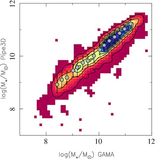
Comparison between the stellar masses derived using the photometric information provided by the GAMA survey and those derived by Pipe3D extracted from the SAMI data cubes.
Due to these differences, we repeated the complete analysis shown in this article using the stellar masses derived by the SAMI galaxy survey. This limits the sample to 993 galaxies, since the filler targets (see Section 2) do not present stellar masses in the SAMI catalogues. Apart from the number of galaxies, we found no significant differences in the results when using the photometric based stellar masses. We do not reproduce all the plots and tables here for the sake of brevity
APPENDIX B: COMPARISON BETWEEN PIPE3D AND LZIFU
In this work, we have used the data products delivered by Pipe3D for the current data set provided by the SAMI survey, a pipeline broadly tested for different IFU data sets, including the ones provided by the CALIFA and MaNGA surveys (e.g. Sánchez et al. 2016b, 2017, 2018) and more complex data sets, like the ones provided by MUSE (e.g Sánchez-Menguiano et al. 2018). However, the SAMI collaboration has developed its own pipeline, LZIFU (Ho et al. 2016), focused on the analysis of multiple components of the emission lines, taking the advantage of the super-high resolution of the SAMI red-arm data sets (although it has been applied to other data sets). The approach of LZIFU is slightly different from the one adopted for Pipe3D. First, the blue and red arms of the SAMI data are combined in order to produce a single spectrum. Then, emission lines are masked, and the stellar continuum is fitted using pPXF (Cappellari 2017). As we showed in Sánchez et al. (2016b) the kinematic analysis provided by pPXF is one of the best, however, the stellar population analysis suffers from both the regularization and the multipolynomial fitting included in the analysis. The approach of using pPXF to derive only the stellar kinematics was adopted by other previous studies (e.g. Sánchez-Blázquez et al. 2014a,,b). For this analysis LZIFU uses the MILES (Sánchez-Blázquez et al. 2006) stellar templates library, with a set of ages and metallicities, comprising a total of 75 individual SSPs.
After subtraction of the underlying stellar population, without a dezonification (the procedure to create a spaxel-wise stellar spectrum model from the spatially binned analysis, e.g. Cid Fernandes et al. 2013; Sánchez et al. 2016b), the emission lines are fitted using a single or multi-Gaussian modelling. The main differences with respect to Pipe3D is therefore: (1) the adopted fitting tool to analyse the stellar population; (2) the adopted SSP-library; (3) the lack of dezonification; (4) the lack of an iterative process of fitting the stellar population, unmasked, once the model of the emission lines is subtracted; and (5) the addition of multi-Gaussian modelling, when required. On top of that, the currently available LZIFU used the SAMI data cubes uncorrected for galactic extinction. Therefore, emission line fluxes should be corrected for that effect. For all these reasons, we have included in here a comparison between the emission line fluxes derived using LZIFU and those derived using Pipe3D, to show the differences.
Fig. B1 shows the comparison between the flux intensities spaxel-by-spaxel derived using LZIFU and Pipe3D for the sub-set of emission lines used in the current study, for the entire analysed data set (i.e. ∼2,000 galaxies), showing the relative difference in the flux intensities compared to the equivalent width of Hα, used as a proxy of the contrast of the emission lines over the continuum. On average, there is a good agreement between both measurements, with the standard deviation of the difference ranging between 25 per cent and 31 per cent for Hα and [S ii] λ6731, respectively, for all the considered values. These differences decrease with the EW(Hα), being of the order of 16 per cent for most of the considered emission lines for EW(Hα) > 30 Å. For the stronger emission lines, in particular for Hα, [N ii] and [O ii] we found no systematic offset between both analyses, with offsets below 1 per cent. The strongest systematic difference is found for Hβ, an emission line strongly affected by the subtraction of the underlying stellar population. For this emission line the offset is of the order of 7 per cent, with Pipe3D deriving larger values than lzifu. A visual inspection of Fig. B1 clearly shows that the main difference is in the regime of the low EWs, i.e, for the retired regions of galaxies, that in any case are not considered in the current study.
![Relative difference between the flux intensities derived for the strongest emission lines in the considered wavelength range as measured by LZIFU with respect to Pipe3D over the EW(Hα) for more than 500 000 individual spectra/spaxels analysed here. Colour maps show the density of points, represented by the black-solid contours (with each contour encircling 95 per cent, 65 per cent, 35 per cent and 20 per cent of the points). The orange solid circles indicate the average value of the relative difference in bins of 0.15 dex in EW(Hα), with the error bars indicating the standard deviation with respect to this mean value. For each emission line a histogram is included showing the distribution of relative differences. From top-left to bottom-right the relative differences are shown for Hα, Hβ, [N ii] λ6583, [O iii] λ5007, [O ii] λ3737, and [S ii] λ6731, as labelled in each panel.](https://oup.silverchair-cdn.com/oup/backfile/Content_public/Journal/mnras/484/3/10.1093_mnras_stz019/1/m_stz019figb1.jpeg?Expires=1750273777&Signature=Fsn8fzdbZETsymeIJOmaHLGL1xiJ~dx0W6ZFr8o4YQxe2nnDuvp-fwA3ddNnBFAr9FcBAjnR9MsPLGFM-~65SSghPSsjKoHDA-uTbo61UvbL9K7~WNMEYiuOavwYpg2jJbMwiMLin9agwt66RpF3Z6kzMMvvvBGxp9vijaWzQVKRqrjBm95BuPNR08g3vbTvgxOcv2gUK6xNOKZ9kjWS0HpyJae0VY~neyIEd5dS9RO2MQNXKyrbiCT58ZHFU~bq0zcZb0FMQI28zMolI6y7yMZAffe~6RUJkIJ-cUUPTWQSUFYlQybdgBSHz46R~J0bUrutBjUAZABacyPMbkGTmA__&Key-Pair-Id=APKAIE5G5CRDK6RD3PGA)
Relative difference between the flux intensities derived for the strongest emission lines in the considered wavelength range as measured by LZIFU with respect to Pipe3D over the EW(Hα) for more than 500 000 individual spectra/spaxels analysed here. Colour maps show the density of points, represented by the black-solid contours (with each contour encircling 95 per cent, 65 per cent, 35 per cent and 20 per cent of the points). The orange solid circles indicate the average value of the relative difference in bins of 0.15 dex in EW(Hα), with the error bars indicating the standard deviation with respect to this mean value. For each emission line a histogram is included showing the distribution of relative differences. From top-left to bottom-right the relative differences are shown for Hα, Hβ, [N ii] λ6583, [O iii] λ5007, [O ii] λ3737, and [S ii] λ6731, as labelled in each panel.
The main goal of the current comparison is to determine how the results are affected by the use of the data products provided by Pipe3D instead of those provided by lzifu. Of the different involved parameters in the current analysis the more sensitive one is the oxygen abundance. A detailed comparison would require that we repeat the full analysis using the new data set, which it is clearly beyond the scope of the current analysis. However, it is still possible to compare the oxygen abundance for the different involved calibrators. Fig. B2 illustrates this analysis, showing the difference between the oxygen abundances derived using the emission line intensities estimated using lzifu and those ones derived using the values provided by Pipe3D, for the O3N2-M13 calibrator, as a function of the EW(Hα), for those spaxels with EW(Hα) > 3 Å (∼200 000 points). We do not include the remaining calibrators since in all the cases we found similar results. Despite the differences reported in the individual emission lines, we found a good agreement in the derived oxygen abundances, with an average systematic offset of ∼0.01 dex, and a scatter of ∼0.07 dex. These offsets decrease to ∼0.005 dex, with a dispersion of ∼0.05 dex for EW(Hα) > 10 Å, i.e. the stronger star-forming regions. These differences are only slightly larger than the nominal errors of the considered oxygen abundances in this article (∼0.03 dex), and clearly lower than the systematic error of the calibrators. As indicated before we found similar results for the remaining calibrators. In summary, we do not consider that our results are significantly affected by the use of either the lzifu or the Pipe3D data products.
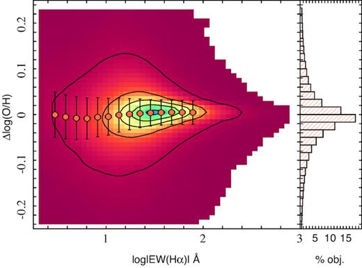
Relative difference between the oxygen abundance derived using the O3N2-M13 calibrator based on the emission line intensities measured by LZIFU with respect to those measured by Pipe3D, plotted over the EW(Hα) for the more than 500 000 individual spectra/spaxels analysed here. Colour map shows the density of points, represented by the black-solid contours (with each contour encircling a 95 per cent, 65 per cent, 35 per cent and 20 per cent of the points). The orange solid circles indicate the average value of the relative difference in bins of 0.15 dex in EW(Hα), with the error bars indicating the standard deviation with respect to this mean value.
APPENDIX C: THE MZ RELATION FROM DIFFERENT IFS GALAXY SURVEYS
We claimed in Section 4.1 and subsequent ones that the MZ relations found using the SAMI galaxy survey data set are similar to that found by previous explorations using other IFS surveys, in particular CALIFA (Sánchez et al. 2017) and MaNGA (Barrera-Ballesteros et al. 2017). It is beyond the goal of the current study to make a detailed comparison between the different results reported using those surveys. However, to illustrate how the different data sets compare to each other, we show in Fig. C1 the MZ-distribution for the t2 calibrator for the three quoted data sets. The values for the CALIFA galaxies were extracted from the published table by Sánchez et al. (2017), which values were derived using the Pipe3D pipeline. On the other hand, the MaNGA data were extracted from the publicly available Pipe3D Value Added Catalogue,4 distributed as part of the SDSS-IV DR14 (Abolfathi et al. 2018). THose are the same date used by Barrera-Ballesteros et al. (2017). As already noticed by Sánchez et al. (2017) the range of stellar masses covered by the three surveys is very similar, despite the fact that the redshift range is considerably more narrow for the CALIFA survey. On the other hand, this survey is incomplete below M* < 109.5M⊙ (Walcher et al. 2014; Sánchez et al. 2016c), a regime much better sampled by SAMI than by any of the other three surveys. Despite these differences, both the distribution of individual points and the mean values in the difference stellar mass bins are remarkably similar, in particular in the mass ranges where the three surveys are complete. Therefore, despite the clear differences in the selection of targets, redshift ranges, coverage of the galaxies and spatial resolutions, when analysed using the same pipeline they produce very similar results.

Mass–metallicity relation derived using the t2 oxygen abundance calibrator for the 1044 galaxies extracted from the SAMI survey analysed in this article (red triangles), together with the same distribution for the 1729 galaxies analysed by Barrera-Ballesteros et al. (2018), extracted from the MaNGA survey (orange circles), and the 612 galaxies analysed by Sánchez et al. (2018), extracted from the CALIFA survey (blue pentagons). Line-connected symbols represent median values at a given mass bin for each different data set, as indicated in the inset, with their average standard deviations represented with an errorbar.
Similar distributions are found for the remaining calibrators included in the current article. We do not include a plot for each of them for the sake of brevity.
APPENDIX D: COMPARISON WITH THE FMR DERIVED USING THE SDSS
We compared the distribution of residuals of the oxygen abundances, after subtraction of the best-fit MZR and pMZR, derived using the adopted calibrators for the sample of galaxies studied in this article with that expected adopting the FMR as described by Mannucci et al. (2010) in Section 4.2. We did that by describing that location in the diagram of residuals as the distribution obtained by subtracting the FMR using the adopted parameterization derived by those authors, from the distribution obtained adopting the pure MZR (Figs. 4 and 8). To justify that this approximation is indeed valid, we explore the same distributions for the SDSS galaxies using the same selection criteria and calibrators presented in Mannucci et al. (2010).
We selected more than 100 000 galaxies from the SDSS DR7 Abazajian et al. (2009), using the values included in the MPA/JHU catalogue, described in Kauffmann et al. (2003) and Brinchmann et al. (2004) following the same criteria listed in Mannucci et al. (2010) (Section 2.1). Those include basically (i) galaxies within a redshift range between 0.07 and 0.3; (ii) with clear detections of the strong emission lines within the considered wavelength range; (iii) with a limit in the dust attenuation; (iv) with line ratios compatible with being ionized by star formation, within the limitations of single-aperture results; and (v) with a compatible measurement of the oxygen abundance using two different calibrators, the one based on the R23 line ratio proposed by Maiolino et al. (2008) (known as M08 in this article), and the one based on the N2 line ratio proposed by Nagao, Maiolino & Marconi (2006). In summary, we mimic as much as possible the selection of galaxies and oxygen abundance derivation described by Mannucci et al. (2010).
Fig. D1 shows the distribution of SDSS selected galaxies following the criteria outlined before in the SFR-M* and M*-O/H diagrams. In general, the distributions are similar to the ones described by Mannucci et al. (2010) (e.g. their fig. 1). In addition, we show the distributions of values extracted from our analysis of the SAMI galaxies, including only star-forming galaxies (according to their sSFR limit adopted in equation (6). We shifted the stellar masses derived for the SAMI survey to consider the differences in IMF and redshift, following the results by Sánchez et al. (2018), considering that Mannucci et al. (2010) adopted a Chabrier IMF (Chabrier 2003), instead of the Salpeter one adopted in the current article, and that the average redshift of the SDSS subsample selected by those authors correponds to the double of that of the SAMI galaxy survey. For the oxygen abundance, we adopted the values derived using the M08 calibrator, which are the most similar ones to those derived by these authors, as indicated before. Once considered those corrections, both samples present similar distributions in the considered diagrams. As expected, the SAMI galaxy survey expands over a wider range of stellar masses, in particular below 109.5, and therefore it samples a regime of lower star-formation rates and lower oxygen abundances. However, for the range in which they overlap they present a very similar distribution in both diagrams.
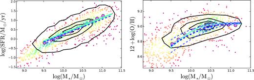
Left-hand panel: Density contourplot of the distribution along the SFR-M* diagram of the SDSS galaxies selected following the criteria described in Mannucci et al. (2010) (black contours), with each contour encircling 95 per cent, 60 per cent, 30 per cent and 10 per cent of the points respectively. The SFR and M* were both extracted from the MPIA/JHU catalogue. The violet solid-circles represent the median value of the SFR in bins of M* of 0.2 dex, ranging between 109.3 and 1011.3 solar masses. The cyan solid line corresponds to the best-fit linear relation between the two quantities, while the dashed-blue line corresponds to the adopted SFMS along this article (extracted from Cano-Díaz et al. 2016). Right-panel: Density contour plot of the distribution along the M*-O/H diagram for the same galaxies shown in the left panel, with the same level for the contours. The oxygen abundance was derived using the prescriptions described in Mannucci et al. (2010), adopting the emission line intensities extracted from the MPIA/JHU catalog. The violet solid circles represent the median value of the oxygen abundances in the same bins described for the left-hand panel. The opaque blue-dashed line corresponds to the expected location of the FMR parameterized as described in Mannucci et al. (2010) (equation (4) of that article) for galaxies following exactly the SFMS, with the two transparent blue-dashed lines indicating the location for galaxies at ±2σ the SFMS. The cyan-solid line corresponds to the MZR estimated by Mannucci et al. (2010) (equation 1 of that article). For comparison purposes, we include the distribution of values for the galaxies observed by the SAMI survey with oxygen abundance derived using the M08 calibrator as solid-circles, whith colour representing the density of points. The stellar masses and SFRs were shifted considering the differences in the IMF and the evolution along the SFR-M* diagram due to the difference in redshift, following the results by Sánchez et al. (2018).
Besides that, we have derived the SFMS (Fig. D1, left panel, cyan-solid line), and we compare it with the parameterization adopted in this article (Fig. D1, left panel, dashed-blue line), finding a very good agreement. Therefore, our parameterization of the SFMS is fully compatible with the sample analysed by Mannucci et al. (2010). In both cases, the dispersion along the SFMS for star-forming galaxies is of the order of ∼0.27 dex, with a very similar fraction of galaxies with SFR larger than 2σ, that range between ∼1.2 per cent (for the SDSS subsample) and ∼2.5 per cent (for the SAMI galaxies).
In the same line, we show that the adopted functional form for the MZR and FMR, as described by Mannucci et al. (2010), describe well the distribution of both SDSS and SAMI galaxies within the M*-O/H diagram. Therefore, they can be used to trace the location of residuals of the oxygen abundance, after removal of the MZR, the parameter Δlog(O/H) shown in Figs. 4 and 8. To demonstrate this more clearly we show in Fig. D2 the distribution of that parameter for the considered subsample of SDSS galaxies as a function of the SFRs and the stellar masses, as a contourplot, together with the same distribution for the SAMI galaxies adopting the M08 calibrator. In addition we show the expected location of the residuals characterized by the subtraction of the FMR, as proposed by Mannucci et al. (2010), to the same functional form assuming no dependence on stellar mass, as described in Section 4.2. It is evident from the figures that the proposed characterization of the effect of the FMR in the distrubution of residuals does actually trace the residuals of the SDSS data set. Confirming indeed the results by Mannucci et al. (2010) for that subsample of galaxies, when adopting the same selection criteria and calibrator. However, when comparing with the same distribution for the analysed SAMI sample, the dependence with the SFR is much weaker than the one proposed by Mannucci et al. (2010). This is particularly evident in the right-hand panel of Fig. D2. Only in the left-hand panel of Fig. D2 we find a weak trend, as already discussed in Section 4.2.
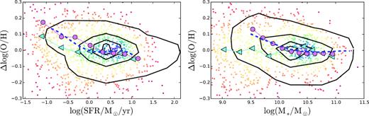
Density contourplot of the distribution residuals of the oxygen abundance, once subtracted the MZR (solid line in Fig. D1, right-hand panel), for the SDSS galaxies selected the criteria described in Mannucci et al. (2010) (black contours), as a function of the SFR (left-hand panel) and the stellar mass (right-hand panel). The violet-solid circles corresponds to the median values of the oxygen abundance residuals for the SDSS galaxies in bins of 0.5 dex and 0.2 dex in SFR and stellar masses, respectively. The blue-dashed line corresponds to the expected residuals once subtracted the FMR relation described by Mannucci et al. (2010) (dashed-blue line in Fig. D1 to the MZR relation described by those authors, for galaxies following exactly the SFMS. It is clearly shown that the blue-dashed line describe very well the average distribution of residuals, represented by the violet-solid line in both panels. For comparison purposes, it was included the distribution of values extracted for the galaxies corresponding to the SAMI survey with oxygen abundance measured using the M08 calibrator as solid-circles, with colours indicating the density of points. The blue-solid triangles correponds to the median values of the residuals of the oxygen abundance for these SAMI galaxies (in the case of the stellar masses, the bins have been increased to 0.3 dex, due to the lower number of objects).
APPENDIX E: DATA SET
The stellar masses, star-formation rates, and oxygen abundances for a sub-set of the 1044 galaxies extracted from the SAMI galaxy survey analysed in the present article are listed in Table E1. The derivation of the different parameters is described in Section 3. For each parameter we include its nominal error, without taking into account the systematic errors of each calibrator, although they have been considered in the analysis. We include in the table the eleven oxygen abundances derived for each galaxy as described in Section 3, for those galaxies for which it was possible to derive this parameter at the effective radius (characteristic oxygen abundance). For those galaxies for which it was not possible to derive one of them we marked the value as a nan. In the case of the oxygen abundances those errors correspond to those derived by the linear regression over the radial distributions. Therefore, they are much smaller than the ones usually derived from studies based on single-aperture spectroscopic data. The full table for the 1044 galaxies is available in electronic format at the following HTTP address: http://132.248.1.15:9154/SAMI/DR_v10/tables/published_table.SAMI.fits.
Stellar Masses, star-formation rates, and characteristics abundances for the all the considered calibrators.
| SAMI | log(M*/M⊙ | log(SFR/M⊙ yr−1) | 12 + log(O/H) | |||||
|---|---|---|---|---|---|---|---|---|
| NAME | O3N2-M13 | N2-M13 | ONS | R23 | O3N2-PP04 | pyqz | ||
| t2 | M08 | T04 | DOP | EPM | ||||
| SAMI105420 | 10.47 ± 0.12 | −2.62 ± 0.06 | nan ± nan | nan ± nan | nan ± nan | nan ± nan | nan ± nan | nan ± nan |
| nan ± nan | nan ± nan | nan ± nan | nan ± nan | nan ± nan | ||||
| SAMI105447 | 10.13 ± 0.15 | −1.38 ± 0.06 | nan ± nan | nan ± nan | nan ± nan | nan ± nan | nan ± nan | nan ± nan |
| nan ± nan | nan ± nan | nan ± nan | nan ± nan | nan ± nan | ||||
| SAMI105519 | 10.50 ± 0.12 | −2.38 ± 0.07 | nan ± nan | nan ± nan | nan ± nan | nan ± nan | nan ± nan | nan ± nan |
| nan ± nan | nan ± nan | nan ± nan | nan ± nan | nan ± nan | ||||
| SAMI105962 | 9.43 ± 0.15 | −0.97 ± 0.07 | 8.33 ± 0.02 | 8.29 ± 0.04 | 8.19 ± 0.06 | 8.39 ± 0.09 | 8.48 ± 0.03 | 8.58 ± 0.06 |
| 8.62 ± 0.05 | 8.63 ± 0.08 | 8.65 ± 0.06 | 8.39 ± 0.11 | 8.51 ± 0.02 | ||||
| SAMI106016 | 10.35 ± 0.12 | −1.50 ± 0.07 | nan ± nan | nan ± nan | nan ± nan | nan ± nan | nan ± nan | nan ± nan |
| nan ± nan | nan ± nan | nan ± nan | nan ± nan | nan ± nan | ||||
| SAMI106042 | 10.29 ± 0.09 | 0.46 ± 0.06 | nan ± nan | nan ± nan | nan ± nan | nan ± nan | nan ± nan | nan ± nan |
| nan ± nan | nan ± nan | nan ± nan | nan ± nan | nan ± nan | ||||
| SAMI106047 | 10.44 ± 0.12 | −0.33 ± 0.06 | 8.47 ± 0.03 | 8.52 ± 0.02 | 8.47 ± 0.02 | 8.47 ± 0.03 | 8.68 ± 0.04 | 9.07 ± 0.05 |
| 8.81 ± 0.02 | 8.91 ± 0.07 | 8.79 ± 0.09 | 9.02 ± 0.07 | 8.45 ± 0.06 | ||||
| SAMI106049 | 9.30 ± 0.14 | −0.90 ± 0.07 | 8.32 ± 0.06 | 8.31 ± 0.06 | 8.17 ± 0.03 | 8.36 ± 0.08 | 8.47 ± 0.08 | 8.57 ± 0.10 |
| 8.62 ± 0.06 | 8.62 ± 0.17 | 8.62 ± 0.14 | 8.38 ± 0.08 | 8.50 ± 0.04 | ||||
| SAMI106065 | 9.02 ± 0.12 | −0.98 ± 0.07 | 8.19 ± 0.05 | 8.12 ± 0.06 | 8.04 ± 0.13 | 8.34 ± 0.04 | 8.27 ± 0.07 | 8.36 ± 0.07 |
| 8.46 ± 0.06 | 8.36 ± 0.10 | 8.64 ± 0.05 | 8.15 ± 0.09 | 8.40 ± 0.06 | ||||
| SAMI106331 | 10.05 ± 0.15 | 0.05 ± 0.07 | 8.30 ± 0.04 | 8.30 ± 0.02 | 8.28 ± 0.03 | 8.41 ± 0.09 | 8.43 ± 0.06 | 8.60 ± 0.05 |
| 8.62 ± 0.04 | 8.70 ± 0.13 | 8.70 ± 0.09 | 8.44 ± 0.07 | 8.42 ± 0.05 | ||||
| SAMI106343 | 9.55 ± 0.14 | −0.67 ± 0.05 | 8.34 ± 0.01 | 8.38 ± 0.01 | 8.35 ± 0.03 | 8.32 ± 0.06 | 8.48 ± 0.02 | 8.74 ± 0.03 |
| 8.67 ± 0.01 | 8.63 ± 0.07 | 8.59 ± 0.08 | 8.51 ± 0.05 | 8.45 ± 0.03 | ||||
| SAMI106376 | 10.63 ± 0.09 | 0.70 ± 0.06 | 8.41 ± 0.03 | 8.44 ± 0.04 | 8.47 ± 0.03 | 8.45 ± 0.01 | 8.59 ± 0.05 | 8.98 ± 0.02 |
| 8.77 ± 0.02 | 8.87 ± 0.07 | 8.83 ± 0.05 | 8.89 ± 0.05 | 8.43 ± 0.04 | ||||
| SAMI106389 | 10.43 ± 0.10 | 0.34 ± 0.07 | 8.50 ± 0.03 | 8.54 ± 0.03 | 8.50 ± 0.02 | 8.45 ± 0.11 | 8.73 ± 0.05 | 9.04 ± 0.02 |
| 8.83 ± 0.04 | 8.86 ± 0.03 | 8.83 ± 0.06 | 9.03 ± 0.09 | 8.52 ± 0.10 | ||||
| SAMI106507 | 10.52 ± 0.13 | 0.49 ± 0.06 | 8.45 ± 0.02 | 8.45 ± 0.02 | 8.49 ± 0.05 | 8.46 ± 0.04 | 8.66 ± 0.04 | 8.96 ± 0.03 |
| 8.79 ± 0.03 | 8.86 ± 0.06 | 8.83 ± 0.06 | 8.81 ± 0.06 | 8.50 ± 0.04 | ||||
| SAMI106549 | 10.59 ± 0.11 | −0.99 ± 0.06 | nan ± nan | nan ± nan | nan ± nan | nan ± nan | nan ± nan | nan ± nan |
| nan ± nan | nan ± nan | nan ± nan | nan ± nan | nan ± nan | ||||
| SAMI106616 | 10.03 ± 0.11 | 0.17 ± 0.06 | 8.40 ± 0.03 | 8.40 ± 0.03 | 8.27 ± 0.20 | 8.43 ± 0.05 | 8.58 ± 0.04 | 8.70 ± 0.12 |
| 8.72 ± 0.04 | 8.72 ± 0.05 | 8.72 ± 0.08 | 8.63 ± 0.12 | 8.50 ± 0.05 | ||||
| SAMI106634 | 10.36 ± 0.12 | 0.36 ± 0.07 | 8.57 ± 0.02 | 8.51 ± 0.01 | 8.60 ± 0.02 | 8.58 ± 0.06 | 8.83 ± 0.03 | 9.12 ± 0.06 |
| 8.91 ± 0.02 | 9.06 ± 0.05 | 9.01 ± 0.10 | 9.12 ± 0.06 | 8.56 ± 0.04 | ||||
| SAMI106638 | 10.58 ± 0.09 | −1.53 ± 0.06 | nan ± nan | nan ± nan | nan ± nan | nan ± nan | nan ± nan | nan ± nan |
| nan ± nan | nan ± nan | nan ± nan | nan ± nan | nan ± nan | ||||
| SAMI106717 | 10.49 ± 0.10 | 0.69 ± 0.06 | 8.52 ± 0.01 | 8.51 ± 0.01 | 8.52 ± 0.04 | 8.53 ± 0.04 | 8.76 ± 0.02 | 9.10 ± 0.01 |
| 8.85 ± 0.02 | 8.93 ± 0.09 | 8.91 ± 0.08 | 8.99 ± 0.05 | 8.53 ± 0.03 | ||||
| SAMI107137 | 10.03 ± 0.09 | −1.47 ± 0.06 | nan ± nan | nan ± nan | nan ± nan | nan ± nan | nan ± nan | nan ± nan |
| nan ± nan | nan ± nan | nan ± nan | nan ± nan | nan ± nan | ||||
| SAMI107214 | 10.08 ± 0.12 | −0.58 ± 0.06 | nan ± nan | nan ± nan | nan ± nan | nan ± nan | nan ± nan | nan ± nan |
| nan ± nan | nan ± nan | nan ± nan | nan ± nan | nan ± nan | ||||
| SAMI107259 | 9.55 ± 0.16 | −0.63 ± 0.06 | 8.36 ± 0.02 | 8.34 ± 0.04 | 8.26 ± 0.05 | 8.42 ± 0.04 | 8.52 ± 0.03 | 8.68 ± 0.07 |
| 8.66 ± 0.03 | 8.73 ± 0.04 | 8.72 ± 0.03 | 8.44 ± 0.09 | 8.51 ± 0.02 | ||||
