


Abstract
We present a morphological and physical analysis of a giant molecular cloud (GMC) using the carbon monoxide isotopologues (12CO, 13CO, C18O 3P2 → 3P1) survey of the Galactic Plane (Mopra CO Southern Galactic Plane Survey), supplemented with neutral carbon maps from the HEAT telescope in Antarctica. The GMC structure (hereinafter the ring) covers the sky region 332° < ℓ < 333° and |$\mathit {b}$| = ±0.5° (hereinafter the G332 region). The mass of the ring and its distance are determined to be |${\sim }2\times 10^{5}\, \mathrm{M}_{\odot}$| and |${\sim }3.7\rm \, kpc$| from the Sun, respectively. The dark molecular gas fraction – estimated from the 13CO and [C i] lines – is |${\sim }17{{\ \rm per\ cent}}$| for a CO Tex between [10,|$20\rm \, K$|]. Comparing the [C i] integrated intensity and N(H2) traced by 13CO and 12CO, we define an X|$\mathrm{_{CI}^{809}}$| factor, analogous to the usual Xco, through the [C i] line. |$X\mathrm{_{CI}^{809}}$| ranges between [1.8,2.0] |$\times 10^{21}\, \mathrm{cm}^{-2}\, \mathrm{K}^{-1}\, \mathrm{km}^{-1}\, \mathrm{s}$|. We examined local variation in Xco and Tex across the cloud, and find in regions where the star formation activity is not in an advanced state, an increase in the mean and dispersion of the Xco factor as the excitation temperature decreases. We present a catalogue of C18O clumps within the cloud, and report their physical characteristics. The star formation (SF) activity ongoing in the cloud shows a correlation with Tex, [C i], and CO emissions, and anticorrelation with Xco, suggesting a North–South spatial gradient in the SF activity. We propose a method to disentangle dust emission across the Galaxy, using H i and 13CO data. We describe virtual reality and augmented reality data visualization techniques, which open new perspectives in the analysis of radio astronomy data.
1 INTRODUCTION
In our Galaxy, as in other galaxies, the space between the stars is filled by a faint medium that consists of ionized, atomic, and molecular gas, high-energy particles (cosmic rays), and dust grains at micron scales. Cosmic rays (CRs), magnetic fields, and the turbulent motion of diffuse gas and dust grains, perturb the interstellar medium (ISM) and contribute to it being inhomogeneously distributed at small scales. The molecular structures within the ISM span a wide range of sizes and masses, from Bok globules (Bok & Reilly 1947) of few solar masses on parsec scales (Clemens, Yun & Heyer 1991), where low-mass stars are born (Yun & Clemens 1990), to immense giant molecular clouds (GMCs) with masses of the order of 104–106 M⊙ spanning tens of parsecs (Bally 1986).
Molecular clouds are the densest and coldest regions of the ISM. Inside them, in regions where CRs, magnetic fields, and violent motions of gas are unable to provide support against gravitational collapse, the molecular gas condenses to form new stars. The ionization and turbulent feedback from the massive newborn stars photodissociates and perturbs the surrounding gas, dissolving the hosting molecular cloud as between 2 and 20 per cent of the original cloud mass is converted into stars (Molinari et al. 2014).
The gas processed by the thermonuclear reactions in the interior of the stars is recycled back into the ISM through mechanisms such as stellar winds and supernova explosions. The injection of matter and energy into the surrounding medium closes the Galactic ecology cycle between the ISM and the stars, continuously enriching the ISM gas reservoir with heavy elements and more complex molecules ready to form a new generation of stars.
The typical time-scale of this cycle is about 5 –10 × 107 yr. With the mean star formation efficiency in GMCs being about 5 per cent, a molecule could exist in the ISM for 1 –2 × 10⁹ yr before being part of a star (Molinari et al. 2014).
The detection of molecular hydrogen (Carruthers 1970) in the far-UV spectrum of a hot star, and the detection of CO (Wilson, Jefferts & Penzias 1970) as the second most abundant molecule in space, started the era of systematic observation of the distribution of interstellar molecules. Although molecular hydrogen is ubiquitously present in the ISM, and is the primary component of GMCs, it is extremely difficult to directly observe. Its lowest transition energy (quadrupole J = 2 → 0 line at 28.22 |$\mu$|m) is at |$510\rm \, K$| above ground (Dabrowski 1984), very far from the typical GMCs temperatures (10–20 |$\rm \, K$|; Goldsmith 1987). The carbon monoxide molecule, having an almost constant relative abundance with respect to H2 (equal to ∼10−4), and a J = 1 → 0 dipole transition at |$5\rm \, K$| above the ground level, is a good proxy for H2 in the environments of interstellar clouds (Scoville & Sanders 1987). The empirical link between the measured quantity, the 12CO line flux, and the H2 column density is the Xco conversion factor (Dame, Hartmann & Thaddeus 2001; Shetty et al. 2011; Bolatto, Wolfire & Leroy 2013) which is typically Xco ≈ 2.0–2.7|$\times 10^{20}\,\mathrm{cm}^{-2}\, \mathrm{K}^{-1}\, \mathrm{km}^{-1}\, \mathrm{s}$| for |$\vert \mathit {b}\vert \lt 1{^{\circ }}$|.
Many experimental observations of the ISM distribution across the Galactic Plane have been made and include the emission in various bands of CO (Heyer et al. 1998; Dame et al. 2001; Mizuno & Fukui 2004; Jackson et al. 2006; Burton et al. 2013; Jones et al. 2013; Barnes et al. 2015; Schuller et al. 2017; Umemoto et al. 2017), H i 21 cm (Gibson et al. 2000; McClure-Griffiths et al. 2001; Stil et al. 2006), methanol masers (Green et al. 2009), HCO+, N2H+, NH3, water maser, and other tracers (Jones et al. 2012; Jackson et al. 2013; Walsh et al. 2014), 1.3 mm continuum (Aguirre et al. 2011), |$870\,\hbox{$\mu $m}$| continuum (Schuller et al. 2009), 350–10|$^4\,\hbox{$\mu $m}$| Planck (Planck Collaboration 2014), 70–500 |$\hbox{$\mu $m}$| Herschel (Molinari et al. 2010), 65–160 |$\hbox{$\mu $m}$| Akari (Ishihara et al. 2010), 3.6–24 |$\hbox{$\mu $m}$| Spitzer (Benjamin et al. 2003; Carey et al. 2009; Gutermuth & Heyer 2015), 3.4–22 |$\hbox{$\mu $m}$| Wise (Wright et al. 2010), and 8.2–21.3 |$\hbox{$\mu $m}$| MSX (Price et al. 2001). The inventory of molecules detected in the ISM ranges from simple ones such as H2O, to organic and more complex molecules such as aldehydes, fullerenes, and polycyclic aromatic hydrocarbon (PAH; Tielens 2013). The ISM is far from being a simple medium.
In the analysis performed in this paper, we will examine in detail the general physical characteristics and the morphology of a GMC recently discovered in the G332 region of the Galactic Plane, identified using data from the Mopra CO Southern Galactic Plane Survey (Braiding et al. 2018).
1.1 Paper structure
In this section, we will give a brief description of how we structured our study. We start with a short presentation of our CO data and the relative reduction pipeline (Section 2), followed by an overview of the CO emission in the G332 sector and the molecular ring cloud (Section 3.1), including how we inferred the cloud distance by solving the kinematic distance (KDA; Section 4). In Section 5.1, we describe the adopted data masking method for creating moment maps (Section 5.1), and the derivation of the CO column density (Section 6) assuming local thermodynamic equilibrium (LTE) conditions. The dust spectral energy distribution (SED) fit and its relative molecular hydrogen column density N(H2), relative to the molecular ring cloud, are described in Section 6.5. In order to investigate the local variation of the Xco factor, in Section 7.1 we compare the 12CO integrated intensity map and N(H2) column density derived from 13CO, at different Tex. Taking advantage of the availability of [C i] line data, we define an X|$\mathrm{_{CI}^{809}}$| factor (Section 7.2) by comparing the molecular hydrogen column density traced by 13CO and 12CO to the [C i] integrated intensity. Moreover, we used the atomic carbon emission, in combination with the 13CO detection, to quantify the dark H2 gas not traced by carbon monoxide (Section 7) and analyse how the [C i] /13CO ratio varies in the ring cloud (Section 8.3). To further inspect the different conditions occurring in the cloud, in Section 9 we describe how we identified clumps and report the C18O principal physical properties in a catalogue (Table A1). In the discussion section we analyse (Section 10.1) how we disentangled the dust emission across the Galaxy with a spiral arm model, while in Section 10.2 we examine the star formation activity ongoing in the cloud. The relation between the measured Xco variation and the physical conditions observed in the cloud are discussed in Section 10.3, and in Sections 10.4 and 10.5, we present ways in which the different physical conditions of the cloud can be inspected using other tracers from CO, such as [C i] and |$8\,\hbox{$\mu $m}$| emission. We end our study (Section 11), presenting new methods based upon virtual reality (VR) and augmented reality (AR) techniques to visualize radio astronomy data, we present three different VR/AR representations in Appendix A.
To help localize the regions of the cloud, single objects, or specific features, we will use the convention shown in Fig. 1. All the global cloud quantities reported in the paper are derived from the region resulting by the union of [SE-R], [SW-R], [W-R], [NW-R], [N-R], and [C-R], if not otherwise stated.
![Summary of the molecular ring divisions, superimposed on a 13CO moment zero map, used here to show morphology. We divided the cloud into parts to examine their typical physical conditions: [N-R] light red, [NW-R] in light orange, [W-R] in blue, [SW-R] in yellow, [SE-R] in violet, and [C-R] in green, here the colours are only for identification purpose. In addition, we use the Galactic coordinate grid as reference: from A to F for Galactic longitude and from 1 to 6 for Galactic latitude, both in steps of 0.15°, for a total of 6 × 6 sub-regions. We use the standard astronomical coordinates convention to localize objects inside each sub-sector; for example, the H ii region in [N-R] will be indicated as [C2-West]. All the figures in this paper use the Galactic coordinate convention as in the figure above, unless otherwise stated. The region in the upper left, in grey, is a superposition between the North–East extremity of the molecular ring and gas that seems to come from the direction of the RCW106 cloud and is not directly connected to the CO ring. The astrophysical objects are plotted using data from simbad (Wenger et al. 2000) database and ds9 software (http://ds9.si.edu/site/Home.html).](https://oup.silverchair-cdn.com/oup/backfile/Content_public/Journal/mnras/484/2/10.1093_mnras_sty3510/1/m_sty3510fig1.jpeg?Expires=1749926495&Signature=GrKAr1ORtqaJRtMMCoTn7B5lOTSsr7ZjGT2Re5q1Y5-GmAEWb7uIvIQGOP4TUEybqVgQcsEu7qz3kCMqcRiIQI9o~DeqHviWgOVdKoEKLg-j5D-HZc204SpKejGd2j01cScLoABS7eDupXnsh-PRNHUzRdKUEA1RDS8EBpk4n86t56uOa7VQyvTEfKtucFQe5dHPyyBor-EUNNEII5PW7y8EVaCIT1KNq4M1OKoGkbjbULLYFI8b9MQNGr5KhaQpOoHlaV7OBxZRZj5VszEtpQSFBf7urnXHfezss4~oqS91uqAjdj0kZM3MXVHUvMfq4b6t91c5XV5kZSHC1aokCg__&Key-Pair-Id=APKAIE5G5CRDK6RD3PGA)
Summary of the molecular ring divisions, superimposed on a 13CO moment zero map, used here to show morphology. We divided the cloud into parts to examine their typical physical conditions: [N-R] light red, [NW-R] in light orange, [W-R] in blue, [SW-R] in yellow, [SE-R] in violet, and [C-R] in green, here the colours are only for identification purpose. In addition, we use the Galactic coordinate grid as reference: from A to F for Galactic longitude and from 1 to 6 for Galactic latitude, both in steps of 0.15°, for a total of 6 × 6 sub-regions. We use the standard astronomical coordinates convention to localize objects inside each sub-sector; for example, the H ii region in [N-R] will be indicated as [C2-West]. All the figures in this paper use the Galactic coordinate convention as in the figure above, unless otherwise stated. The region in the upper left, in grey, is a superposition between the North–East extremity of the molecular ring and gas that seems to come from the direction of the RCW106 cloud and is not directly connected to the CO ring. The astrophysical objects are plotted using data from simbad (Wenger et al. 2000) database and ds9 software (http://ds9.si.edu/site/Home.html).
2 OBSERVATIONS AND DATA REDUCTION
2.1 CO, [C i], and H i
In this paper five spectral lines will be considered: the three CO isotopologues 12CO, 13CO, C18O J = 1 → 0 transition (hereinafter called simply 12CO, 13CO, and C18O), the atomic carbon [C i] 3P2 → 3P1 transition line at 809.342 GHz (hereinafter [C i]), and the H i 21 cm line.
The CO lines come from the isotopologue survey of 12CO, 13CO, and C18O, J = 1 → 0 transition lines (30 arcsec pixel size and |${\sim }0.1 \rm \, km\, s^{-1}$| spectral resolution), obtained using the 22|$\rm \, m$| single dish Mopra millimeter wave telescope, part of the Mopra Southern Galactic Plane CO Survey of the Milky Way (Burton et al. 2013, 2014; Braiding et al. 2015; Rebolledo et al. 2016; Blackwell, Burton & Rowell 2017; Braiding et al. 2018). In this survey we used the fast-on-the-fly mapping that maps the four CO isotopologues at the same time, taking 8 × 256 ms samples each cycle (2.048 s). In Galactic coordinates it covers |$\vert \mathit {b}\vert \lt 1^{\circ}$| and 265° < ℓ < 10°, each square degree is divided into 20 rectangles of 60 arcmin × 6 arcmin, 10 aligned along lines of Galactic longitude, and 10 aligned with Galactic latitude. Each stripe required ∼1 h to be completed, at a scanning speed of ∼30 arcsec s−1. The CO data presented in this paper, relative to the G332 region, was taken during the first half of 2012 June. The C17O line was included in the survey but did not show any detectable emission and will be not considered further.
The [C i] data (72 arcsec beam FWHM, pixel size of 2 arcmin and |$0.5 \rm \, km\, s^{-1}$| spectral resolution) comes from the High Elevation Antarctic Telescope HEAT1 (Kulesa 2011; Burton et al. 2015) located at Ridge A, a deep-field site close to the highest dome on the Antarctic plateau, |${\sim }1000\rm \, km$| from the South Pole Station.
The H i data come from the Parkes+ATCA Southern Galactic Plane Survey (SGPS, McClure-Griffiths et al. 2005) and has a voxel size of 40 arcsec and a spectral resolution of |$0.8\rm \, km\, s^{-1}$|. Table 1 summarizes the characteristics of the surveys we have used.
Parameters for the data sets. The 1σ rms noise for the CO data was derived from the velocity interval between −490 and |$-186.5\rm \, km\, s^{-1}$| in which no emission was detected. For the H i and C i lines we used −186.3 to |$-135.5\rm \, km\, s^{-1}$| and −134 to |$-120\rm \, km\, s^{-1}$|, respectively. For CO the rms is in uncorrected |$\mathrm{T}_{\mathrm{A}}^*$||$\rm \, K$| units.
| Survey | Tracer | Frequency (GHz) | Pixel size (arcsec) | Velocity range (km s−1) | Δv (km s−1) | 1σ (K) rms |
|---|---|---|---|---|---|---|
| MopraCO | 12CO J = 1–0 | 115.271 | 30 | −500 to +500 | 0.092 | 1.47 |
| 13CO J = 1–0 | 110.201 | – | −500 to +240 | – | 0.70 | |
| C18O J = 1–0 | 109.782 | – | −500 to +230 | – | 0.77 | |
| HEAT | C iJ = 2–1 | 809.342 | 72 | −134 to +19 | 0.500 | 0.12 |
| SGPS | H iS = 1–0 | 1.420 | 40 | −202 to +142 | 0.824 | 1.60 |
2.2 CO data reduction
Here is given a brief description of the pipeline used to reduce CO data. The raw data in rpfits2 format are processed using livedata3 to subtract the reference position emission. An idl4 routine then flags bad data values above a given threshold (usually 5σ). Data are then gridded using the gridzilla3 package and cleaned again using routines in idl. The original data reduction pipeline, described in Burton et al. (2013), is used in this work with the only addition of the flagging routine between the livedata and gridzilla steps. The final output is a square degree fits datacube with angular dimensions of 131 × 131 pixels, and a velocity range of (|$-582 \rm \, km\, s^{-1}$| to |$500 \rm \, km\, s^{-1}$|), (|$-510 \rm \, km\, s^{-1}$| to |$245 \rm \, km\, s^{-1}$|) and (|$-515 \rm \, km\, s^{-1}$| to |$215 \rm \, km\, s^{-1}$|) for 12CO, 13CO, and C18O, respectively. All the CO datacubes were then regridded, using the miriad5 command regrid6, to the C18O grid, which is (marginally) the coarser spectral resolution compared to 12CO. The final carbon monoxide datacubes have is composed by voxels an angular voxel dimension of 30 arcsec and a spectral resolution of |$0.092\rm \, km\, s^{-1}$|.
2.3 Near and far-infrared emission
To correlate our CO data to dust emission we used two surveys of the near-infrared emission coming from the G332 sector: the Galactic Legacy Infrared Midplane Survey ExtraordinaireGLIMPSE (Benjamin et al. 2003; Churchwell et al. 2009) and the |$24\,\hbox{$\mu $m}$| band MIPSGAL (Carey et al. 2009; Gutermuth & Heyer 2015) observed by the Spitzer space telescope.7 On the longer wavelength side, to derive the cold dust emission temperature profile, we considered the Herschel Infrared Galactic Plane Survey (Hi-GAL, Molinari et al. 2010), which is an Open Time Key Project of the Herschel Space Telescope covering the Galactic Plane in a 2° wide strip (|$\vert \mathit {b}\vert \lt 1^{\circ}$|) in five photometric bands centred at |$70, 160, 250, 350,\ \text{and}\ 500\,\hbox{$\mu $m}$|.
3 THE G332 REGION
The H i and 13CO average emission spectrum coming from the whole G332 square-degree sector is shown in Fig. 2, together with Gaussian curves used to fit the CO emission along the line of sight (see Table 2 for line parameters). The Gaussian curves were obtained using the scouse8 software (Henshaw et al. 2016).
![Left-hand image: Average spectral profile plot along the VLSR interval $[-105,-10]\rm \, km\, s^{-1}$ of $\mathrm{T}_{\mathrm{A}}^*$13CO (black curve) and H i (blue dashed curve) for the entire G332 square-degree sector, which encloses the region shown in Fig. 1. H i is in Tmb units and reduced by a factor of 200. The red curve is the sum of seven Gaussian curves (displayed in different colours) derived from the multi-Gaussian fit of the 13CO average emission. See Table 2 for the parameters of each fit. Right-hand image: 2D heat map scatter plot comparing the second moment map (velocity dispersion) versus the first moment map (velocity centroid) of each line of sight belonging to the 13CO datacube, binned by four channels along the velocity axis in the same velocity range as considered in the left-hand panel.](https://oup.silverchair-cdn.com/oup/backfile/Content_public/Journal/mnras/484/2/10.1093_mnras_sty3510/1/m_sty3510fig2.jpeg?Expires=1749926495&Signature=togh3lZ-LQaWGe657-Bf99Mx~yW~5RL8YQ7-n1udWzqoI5IYu9PF7vmNxTu03FAxus3wu39M2rc5VuKkm8NZ~jsbOFccldYagv7KFAPhSWueBeUtfm7qlMFkCP61FhC0rRvb2lBHFN3IBMDoBJejj524x1E9RnJB43YRRDvQJ3b6hXPjkLD-XQdtH5gq2FpZRVglry7lP4DEHKP19ghFtcS1~bs69HlqO-AFF2tskGsz9M1Oe6U1U~4ojwkdacRY0cBc66wrar16WGePAke4FHplZFUd6kwct-DArT~8CO~diR4mokMXzzjQTLQe6olMzobF1tyHYeM5kB0B~YQx2w__&Key-Pair-Id=APKAIE5G5CRDK6RD3PGA)
Left-hand image: Average spectral profile plot along the VLSR interval |$[-105,-10]\rm \, km\, s^{-1}$| of |$\mathrm{T}_{\mathrm{A}}^*$|13CO (black curve) and H i (blue dashed curve) for the entire G332 square-degree sector, which encloses the region shown in Fig. 1. H i is in Tmb units and reduced by a factor of 200. The red curve is the sum of seven Gaussian curves (displayed in different colours) derived from the multi-Gaussian fit of the 13CO average emission. See Table 2 for the parameters of each fit. Right-hand image: 2D heat map scatter plot comparing the second moment map (velocity dispersion) versus the first moment map (velocity centroid) of each line of sight belonging to the 13CO datacube, binned by four channels along the velocity axis in the same velocity range as considered in the left-hand panel.
Parameters for the seven Gaussian fits of the average 13CO emission in the G332 sector (as shown in Fig. 2). The third column is the Full Width at Tenth of Maximum FWTM. The average emission peak is in uncorrected |$\mathrm{T}_{\mathrm{A}}^*$|.
| Velocity centroid | FWHM | FWTM | Peak (|$\mathrm{T}_{\mathrm{A}}^*$|) |
|---|---|---|---|
| (km s−1) | (km s−1) | (km s−1) | (K) |
| −101.74 ± 0.54 | 9.52 ± 0.82 | 17.43 | 0.12 ± 0.01 |
| −95.10 ± 0.20 | 5.78 ± 0.58 | 10.55 | 0.15 ± 0.03 |
| −88.73 ± 0.32 | 9.23 ± 0.47 | 16.90 | 0.23 ± 0.01 |
| −68.10 ± 0.15 | 6.79 ± 0.57 | 12.40 | 0.15 ± 0.02 |
| −57.63 ± 0.31 | 14.70 ± 2.53 | 26.85 | 0.21 ± 0.01 |
| −49.98 ± 0.04 | 4.85 ± 0.16 | 8.85 | 0.37 ± 0.02 |
| −42.37 ± 0.14 | 9.10 ± 0.19 | 16.60 | 0.33 ± 0.01 |
The right-hand panel in Fig. 2 is a 2D heat map scatter plot9 between the gas velocity dispersion and the first moment map, computed along the interval |$[-115,-10]\rm \, km\, s^{-1}$|. The pixel distribution shows a branching pattern that is visible at coordinates around |$[22,-70]\rm \, km\, s^{-1}$| and has nodes at |$[12.5, -85]\rm \, km\, s^{-1}$| and |$[10,-50]\rm \, km\, s^{-1}$|.
Few pixels have the largest velocity dispersion with velocity centroid in the interval −60 <VLSR|$\lt -80\rm \, km\, s^{-1}$|, while most of the emission has a second moment below |$10\rm \, km\, s^{-1}$| and a first moment constrained to −55 <VLSR|$\lt -40\rm \, km\, s^{-1}$|. Small localized 12CO and 13CO emissions, missing in the square-degree average profile (Fig. 3), were detected at positive velocities |${\sim }5\rm \, km\, s^{-1}$| and at |${\sim }-20\rm \, , -7\rm \,$|, and |$0\rm \, km\, s^{-1}$|, but this will not be considered in our analysis.
![Average CO, H i, and [C i] spectral profiles for the ring region shown in Fig. 1. This differs from Fig. 2 in considering the sky region 332.1° < ℓ < 332.8° and −0.30° < b < 0.45°. The two vertical red lines indicate the spectral interval in which the molecular ring is identified. H i and 12CO are plotted reduced by a factor of 100 and 3, respectively, to allow a clear comparison with other lines. The CO and [C i] peak is at VLSR${\approx }-50\rm \, km\, s^{-1}$, while, at the same velocity, H i presents a local minimum.](https://oup.silverchair-cdn.com/oup/backfile/Content_public/Journal/mnras/484/2/10.1093_mnras_sty3510/1/m_sty3510fig3.jpeg?Expires=1749926495&Signature=JRsxdHV7DuiG1F1-~-DhPlk5DqVtHdf4xxFbdeFJIlAIbpmyEk-QDvVCaF2cCobLHzq3Lwn9xJGRP4YZVT21-lyOTOsuQgJfYAGjadbMLBzTsBDm8fQM8DguqcpeyspGUDwJaL1Mjx9NkHIV-j0PMmlS~D9YdlmFdPnqsJRFxMtorgiR3r8P66vZWp~ZeXnf7rGVKM0cFeNUIh6KsntYtPJQ7U6xj7JCEoWNNGTF~fDZnRnwcStc6TxeP6pxl596QAVm5gQlZy0aBUdpY4jlTmo~41g2f-oj3Qkp3ZFtqxOa2Xf3qj-jM4ffRzz5W9T2WyTU~zhlaKnyj1IwXU9z2Q__&Key-Pair-Id=APKAIE5G5CRDK6RD3PGA)
Average CO, H i, and [C i] spectral profiles for the ring region shown in Fig. 1. This differs from Fig. 2 in considering the sky region 332.1° < ℓ < 332.8° and −0.30° < b < 0.45°. The two vertical red lines indicate the spectral interval in which the molecular ring is identified. H i and 12CO are plotted reduced by a factor of 100 and 3, respectively, to allow a clear comparison with other lines. The CO and [C i] peak is at VLSR|${\approx }-50\rm \, km\, s^{-1}$|, while, at the same velocity, H i presents a local minimum.
3.1 The G332 giant molecular ring morphology
The average spectral profiles of the CO lines, and [C i], show a peak (left-hand panel of Figs 2 and 3) at VLSR = |$-50\rm \, km\, s^{-1}$|, where a molecular cloud is seen in both atomic and molecular carbon. In order to identify the feature linked to it, we investigated the emission distribution and produced a 3D model10 of the 13CO datacube between |$-55\lt \text{$V_{\mathrm{LSR}}$ }\lt -30\rm \, km\, s^{-1}$|.
Inspection of the CO spectral line and the sigma threshold masks (see Section 5.1) led us to focus our study on Galactic coordinates 332.0 < ℓ < 332.8, −0.3 < b < 0.4, within which we identified the principal emission structure (the ring), and on the velocity range |$-55 \lt \text{$V_{\mathrm{LSR}}$ }\lt -44\rm \, km\, s^{-1}$| (which we refer to as the ring velocity range). This choice was made to prevent contamination coming from gas not evidently connected to the ring or with a very low signal-to-noise ratio.11 The extent defined above is the same used to compute moment maps (as the moment zero in Fig. 4) and all the plots belonging to the ring, unless otherwise specified.
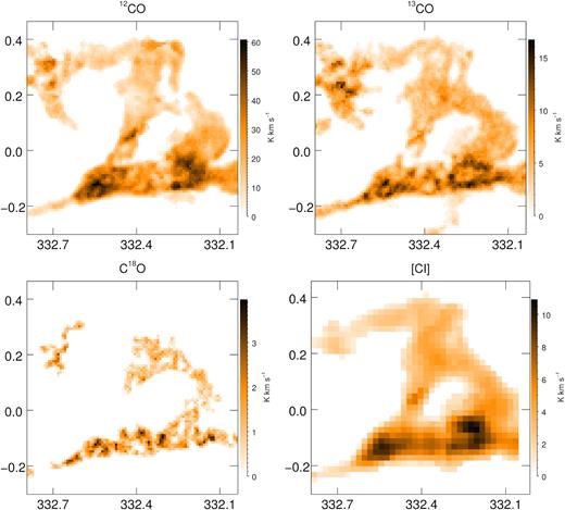
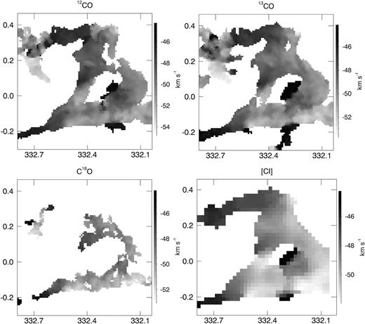
Integrated intensity maps of CO lines (|$\mathrm{T}_{\mathrm{A}}^*$|) and C i (Tmb) over the velocity range |$-55\, \mathrm{km\, s}^{-1} \lt$|VLSR|$\lt -44\, \mathrm{km\, s}^{-1}$|. Axes are Galactic with the x and y indicating longitude and latitude, respectively.
The region delimited by coordinate ℓ > 332.6° and |$0.4^{\circ }\lt \mathit {b}\lt 0.15^{\circ}$| (see Fig. 1), where the North–East extremity of the ring and another cloud extremity coming from the East fall in the same ring VLSR range, is excluded from our study, since the two clouds cannot be clearly separated.
Taking into account the above mentioned constraints, the ring angular dimensions are about 0.8° along both South–North and East–West directions, showing mean velocity FWHMs approximately equal to 9, 5, 4, and |$8.5\rm \, km\, s^{-1}$| for the 12CO, 13CO, C18O, and [C i] average line profiles, respectively.
4 THE KINEMATIC DISTANCE AMBIGUITY
We estimated the distance of the ring by using the Galactic rotation model from McClure-Griffiths & Dickey (2007), resolving the KDA by comparing the SGPS HI survey data to the Mopra CO and HEAT surveys. Velocities profiles in Fig. 3 show a local H i minimum in correspondence of CO and [C i] peaks at around |$-50\rm \, km\, s^{-1}$|. Inspecting the CO and H i spectral lines we found a clear decrease in H i where CO peaks, for all of line of sights passing through the ring, indicating the presence of a cold atomic component at the same velocity of the CO peak. This strengthens the interpretation of the ring as a unique connected structure. The near distance solution for VLSR = |$-50\rm \, km\, s^{-1}$|, using a ring geometrical centre (ℓ, b) = (332.3°, 0.0°), is |${\sim }3.73\rm \, kpc$| from the Sun. Assuming the Galaxy model of Vallée (2014), this distance places the molecular ring inside the Scutum-Crux arm (Fig. 5). For comparison we also used the Bayesian approach12 of Reid et al. (2016) that gave a distance of |$3.22\pm 0.44\rm \, kpc$|. However, in our analysis we will adopt the 3.73 kpc value.
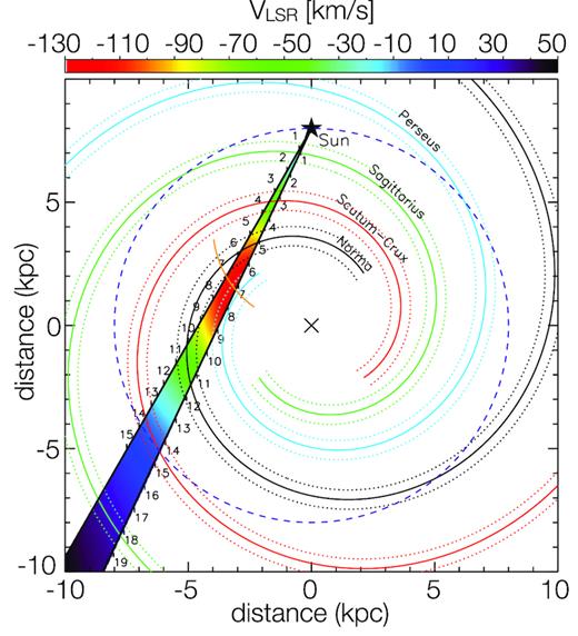
Colour representation of the Galactic velocity field for the 330°–335° longitude range, based on the rotation curve and Galaxy model described in Section 4. The numbers along the line of sight indicate the distance from the Sun in kpc. The Solar circle is indicated by the dashed circle while the orange arc indicates the tangent points to the spiral arms.
In Fig. 6 we present the Galactic spiral arms overplotted with the Position Velocity (PV) image of the 12CO average emission from the region shown in Fig. 1. It is seen that most of the CO is constrained inside the Norma near, Norma far, and Scutum-Crux near arms, while in the Sagittarius near and Scutum-Crux arms, there are only a few small clouds. The position ambiguity between Scutum-Crux near and Norma far is clearly visible as they are superimposed.
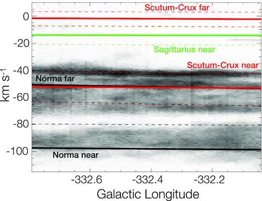
PV spiral arms plot, based on the Galactic rotation curve and Galaxy model as described in Section 4, over the 12CO average intensity PV plot image. The solid lines represent arm mean positions, while segmented lines represent their outer edges. The colour codes for the spiral arms are the same as in Fig. 5.
The analysis of the 12CO spectral lines revealed emission peaks between |$-20\rm \, km\, s^{-1}\lt$|VLSR|$\lt 0\rm \, km\, s^{-1}$|, coming from small weak clouds apparently localized in the Scutum-Crux far arm and in the Sagittarius near arm. Nevertheless, no local H i minimums are present at the same VLSR of these 12CO peaks, suggesting a far distance solution for their KDA of the order of |${\sim }14\rm \, kpc$|.
5 MOMENT MAPS
5.1 Mask for the moment maps
To improve the detection of the faintest CO emission (as in the case of C18O), we used the miriad task imbin13 to bin the original datacubes along the velocity axis by a factor of 4, consequently degrading the spectral resolution to |${\sim }0.35\rm \, km\, s^{-1}$|. To separate real emission from noise we applied, on the binned cubes, a custom idl routine based on the method described by T. M. Dame.14 Selecting the velocity range, and the spatial region, the extracted cube is 3D smoothed by a boxcar average of a certain width.15 For CO and [C i] we used a boxcar kernel width of [3,3,2] voxels: the average is computed considering three voxels in each angular direction and two along the spectral axis. The rms noise of the smoothed cube, σs, is used to select only voxels above a σdet = σs × ϕdet threshold. The selection is then expanded including all the surrounding voxels above the σext = σs × ϕext level. This growing mask procedure is similar to the masking method used in the cprops algorithm (Rosolowsky & Leroy 2006). Both the selection and the expansion steps are done on the smoothed cube. All voxels that pass these two criteria form the mask applied to the original cube to compute the moment maps. For 12CO, 13CO, and C18O the chosen masking threshold values are [6,3], written in the form [ϕdet, ϕext]. In this paper we will always refer to this kind of 3D mask coming from a four-channel binned datacube (specifying from which line originates), if not otherwise stated. The same values of smoothing and threshold are used for [C i] and HI. In Fig. 4 are shown the resulting moment maps for CO and [CI]. We opted a boxcar instead of a Gaussian smooth after performing a series of tests applying a custom genetic algorithm (Holland 1992) to find the best combination of the two threshold and two smoothing parameters.
To simplify the description of this algorithm we will take advantage of terms usually used in genetics. The algorithm basically creates a certain number (population) of moment map individuals from a different choice of the above mentioned four parameters (four genes or genotype), randomly selected from a defined range. To each map (individual) is assigned a score through a custom defined function (fitness function). In our definition the best individuals have the higher fitness function. This function takes into account the number of voxels with negative values included in the 3D mask, the number of voxels of the mask, the number of negative and positive pixels in the final zeroth moment map. In detail, the fitness function is defined as ffit = (P+/1000 − P−) + (V+ − V−)/VN, where P+ and P− are, respectively, the number of positive and negative value pixels in the resulting 2D zeroth moment map, while V+, V−, and VN are, respectively, the number of positive, negative, and total voxels included in the 3D mask. The major weight given to P−, with respect to P+, is to greatly decrease the fitness function for individuals having negative value pixels in the final zeroth moment map. As a consequence, these individuals will have minimal chances of passing their genotype to the next generation. The parameters (genotype) of the elements of the population with the best score are mixed together (crossover) to create a new set of parameters (sons genotype) introducing a small mutation (mutation), thus creating a second generation of the parameter set. When the maximum value of the fitness function does not change for a certain number of iterations, prior to stopping the process, the algorithm increases the variation in the sons parameters (mutation amplification) for a maximum number of iterations, in order to prevent the algorithm stopping on a local maximum, exploring a wider parameter space. If a new individual is found the process continues with the mutation rate set to the initial value.
The integrated flux coming from the masked cubes was found to be the |$51$|, |$70$|, and |$55{{\ \rm per\ cent}}$| of the integrated flux coming from the non-masked cubes, respectively, for the 12CO, 13CO, and C18O lines.
Comparing the 12CO and the 13CO integrated intensity maps, it is possible to see regions in which there is no 12CO counterpart of 13CO emission, in particular around (ℓ, b)∼(332.3°, 0.2°). This apparent cavity in [NW-R] is close to PLW2012 G332.277+00.189-048.9 (Purcell et al. 2012), a dense core at (ℓ, b,) ≈ (332.274°, 0.187°). This is a threshold effect of the 3D mask: in this region 12CO emission in the smoothed cube is below the masking threshold while 13CO is above. Examining the line profile (Fig. 7) this behaviour can be explained as 12CO self-absorption, since the local minimum of the 12CO spectral lines is close to the 13CO and C18O local peaks. However, a deeper inspection of all the ring 12CO spectra reveals that this effect is limited to few lines of sight, mainly distributed in the Northern part of the ring, besides the above mentioned region.
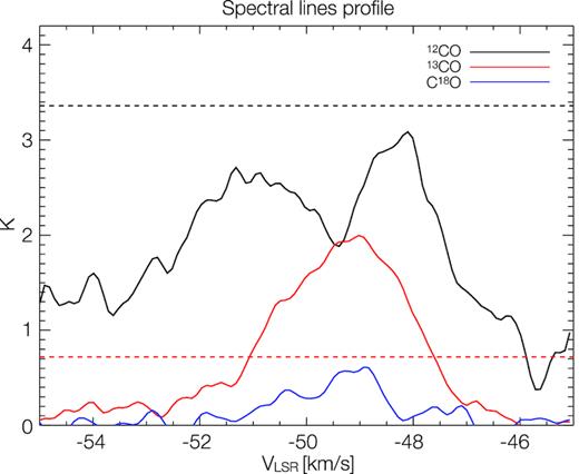
Single pixel spectral line profile of the line of sight (ℓ, b) ≈ (332.3°, 0.2°). 12CO shows self-absorption, while the 13CO and C18O show a peak close to a 12CO minimum. In black is 12CO while in red and blue are 13CO and C18O, respectively. The two dotted horizontal lines represent the 3σ threshold (black for 12CO and red for 13CO) used to derive the mask for the moment maps. The 12CO is thresholded out even though its emission is stronger than 13CO.
5.2 Integrated intensity
Integrated intensity maps of [C i] and all CO lines are shown in Fig. 4. All the lines show the ring shape, with 12CO, 13CO, and [C i] being most similar in shape. Thicker structures seen in C18O are distributed along an arc-like structure interrupted by a few cavities. Here we will briefly describe the main features:
12CO, 13CO, and [C i] are higher in [C-R], [SE-R], and [SW-R]. The first region covers a system of multiple bubbles [CPA2006] S52 that encloses [CPA2006] S53, and [SPK2012] MWP1G332437+000547 (Churchwell et al. 2006; Simpson et al. 2012), presenting a bright |$8\,\hbox{$\mu $m}$| emission enclosing diffuse |$24\,\hbox{$\mu $m}$| emission and no significant C18O detection.
[S-R] and [SW-R] host H ii regions (Urquhart et al. 2014; see Fig. 1) with velocities compatible with the ring velocity interval: AGAL332.544-00.124 at VLSR = −46.7 km s−1, close to the highest 12CO integrated emission and AGAL332.296-00.094 at VLSR = −48.2 km s−1, near to a 13CO and a C18O integrated emission peak.
13CO and C18O maximum integrated emission is at (ℓ, b)∼(332.40°, −0.09°), close to a radio sub-mm source AGAL G332.389-00.091 (Contreras et al. 2013) and a Young Stellar Object (YSO) candidate SSTGLMC G332.3810-00.0992 (Robitaille et al. 2008).
C18O distribution presents a number of dense spots in the southern part, in which there are prestellar and protostellar cores ([SE-R]) as well as dense cores ([SW-R]). The [N-R] shows lower emission, but as in the southern regions there are some YSO candidates (see Fig 1).
The major contribution to the overall ring emission comes from the southern ring that seems to hosts more sites of star formation activity (see Section 10.2) compared to [N-R], [NW-R], and [W-R] regions. As expected, among all the CO lines, 12CO emission is the most widespread. The apparent absence of 12CO emission in [NW-R] where 13CO is present is explained in Section 5.1.
5.3 Ring velocity field
The ring velocity field is shown in Fig. 8. The Southern ring emission comes mainly from VLSR|$=-50\rm \, km\, s^{-1}$|, and is |$3\, \mathrm{ to} \, -4\rm \, km\, s^{-1}$| wide (see Fig. 9). The Eastern part of [SE-R] has velocity centroid shifts of about |$+5\rm \, km\, s^{-1}$| reaching VLSR|$=-44\rm \, km\, s^{-1}$| for all the lines, equal to a velocity gradient of |$0.30\rm \, km\, s^{-1}\, \mathrm{pc}^{ -1}$|. In the same way, the [C1] region shear is about |$0.28\rm \, km\, s^{-1}\, \mathrm{pc}^{ -1}$|.
Velocity centroid maps of the emission for each line derived from the first moment map.
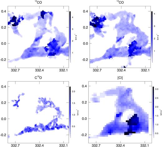
Velocity dispersion distribution of the molecular ring for the four emission lines derived from second moment maps.
[N-R] and [W-R] are sheared by about |${\sim }2\rm \, km\, s^{-1}$| with respect to the Southern part. Differently from [W-R], in which the velocity field is almost constant at VLSR|${\approx }-50\rm \, km\, s^{-1}$|, [SW-R] has a more complex velocity field, which can be related to the objects in the regions (see Fig. 1).
In [C-R] the first moment map shows a rapid shift of about |$5\rm \, km\, s^{-1}$|; as said in Section 5.2, this region is associated with many bubbles. Here, 12CO and 13CO have broader emissions (see Fig. 9) and show spectral lines in which it is possible to identify two peaks separated by a ΔVLSR|${\approx }5.5\rm \, km\, s^{-1}$|.
At coordinates (ℓ, b) = (332.4°, 0.16°) a velocity gradient ΔVLSR = 1.5 |$\rm \, km\, s^{-1}$|, 3 arcmin in diameter, is only visible in 12CO and 13CO emissions, and the [C i] resolution is insufficient to distinguish it. In the literature (Peretto & Fuller 2009) are reported two dark clouds close to this position SDC G332.383+0.182 and G332.419+0.174 and Beichman et al. (1988) an IR source IRAS 16111-5032. In the same position, 12CO and 13CO spectral lines indicate a dip in the 12CO emission in correspondence of a 13CO peak, a scenario compatible with 12CO self-absorption.
Comparing the first (Fig. 8) and the second moment maps (Fig. 9) it is possible to identify, for all the spectral lines except C18O, sharp value changes in [D4] and [D6]. This can be explained as a partial superimposition of cloud fragments detected at a VLSR greater than the main ring VLSR . The second moment maps (Fig. 9) show a pattern in [SW-R] that confirms this interpretation: an increase in the velocity dispersion where the first moment maps are suggesting the superposition between the fragments and the ring emission. The same explanation applies to 12CO in [D1], where both the first and second moment maps show a sharp change in value. In this case, the 12CO emission of the ring cloud is extended towards lower velocities.
To better understand the physical connection between these extensions and the main ring, we made use of VR and AR representations10 (described in Appendix A), which allows us to consider them as part of the ring complex.
6 CO AND [C i] COLUMN DENSITY AND OPTICAL DEPTH
In order to take in account the response of the Mopra radio telescope, the measured signal (|$T_{A}^{*}$|) was converted into the corrected brightness temperature TMB, using the extended beam efficiency ηxb = 0.55 at 115 GHz (Ladd et al. 2005), since the sources considered in this work are more extended than the Mopra main beam. The HEAT datacube is in Tmb. In Fig. A1 we report the column density maps derived for 13CO, C18O, and [C i] using different Tex values. Our approach to derive 12CO, 13CO, C18O, and [C i] column densities is based on assuming LTE conditions, and same LTE temperature for all the CO isotopologues. It is important to note that the latter assumption is not verified in the presence of temperature gradients.
Besides LTE conditions, we considered a beam filling factor equal to unity, optically thick 12CO, and optically thin 13CO and C18O emissions. The last hypothesis was verified by inspecting voxel-by-voxel the C18O/13CO ratio, which was found to be in the range [0.2–0.25] in regions where the C18O is bright enough to yield a significant ratio value within the noise level. It is important to note that this ratio depends also on the oxygen 18O abundance relative to 16O as well.
In the next paragraphs we describe in detail all the steps followed to compute optical depth and column densities.
6.1 13CO and C18O
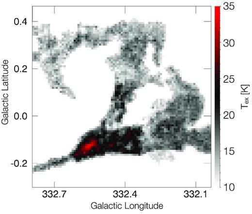
Map of Tex as derived from the 12CO peak emission for each line of sight. The maximum value is ∼35 K.

We applied the same approach used for 13CO to the C18O column density and optical depth computation. To derive the relative column density, we adopted the value from Frerking et al. (1982) of |$\mathrm{[H_{2}/C{^{18}}O]}=5.88\times 10^6$|, an order of magnitude less abundant than 13CO.
6.2 12CO to H2 column density
6.3 [CI] 3P2 → 3P1
![Map of [C i] optical depth peak values for each line of sight, derived for a Tex = 30 K. The highest values are in correspondence of the highest Tex derived from the 12CO peak emission, as shown in Fig. 10, and of the highest dust temperature as plotted in Fig. 11.](https://oup.silverchair-cdn.com/oup/backfile/Content_public/Journal/mnras/484/2/10.1093_mnras_sty3510/1/m_sty3510fig12.jpeg?Expires=1749926495&Signature=yegBEg-J4a66oQJiCjBDn9oVVTFrBSnzXdF5HrWM5Vd2ZGVRuhw51F6GFc0tbiB-uA6rxNW4rclRl0HoUrqIPzKGc4G0b1IioIiB9KUGbGblqKthlT0Zts28Sq88t6pIqZlfixg5B7t4gm1JwyvgmroO~aE~8f8R4QHmvz5YWwFvj4hxSEae4cCyHNMxHbZLJcVGWVNIVZKrA3MJ-P6Co70jVkQvco70L5C4dEvfxgfgHI5dXdWhkeJ3cJHGhY7xK4hOhZB3rwR4PeaXzwdDfS6tyL-kyWUwUp8zYojg52zzWSNV2W0jWHOA-Q37ihML5zbqVIAR3NUWvzUc52XSlA__&Key-Pair-Id=APKAIE5G5CRDK6RD3PGA)
a = 16.51
b = 7.12 × 10⁻²
c = −17.44
We followed the same method used in the CO optical depth calculation shown in equation (4). Differently to CO we choose two a priori excitation temperatures: Tex = 30 and 50 K, both of them higher than the typical CO Tmb to take into account that [C i] exists in warmer physical conditions (e.g. the surface regions of molecular clouds, or in the neighbourhood of intense radiation sources). We find comparing to Tex = 50 K, N(CI) increases by a factor of ∼4 and decreases by |${\sim }70{{\ \rm per\ cent}}$|, when using Tex = 20 and 80 K, respectively.
Inspecting the [C i] data we found that the emission is coming from both the external layers around the ring and from the inner part, in a web pattern, in particular in the southern ring. This indicates that localized sources of Far-UV (FUV) radiation are present in the cloud interior. In Section 10.2 we will discuss further the behaviour and interpretation of the [C i] emission.
6.4 Column density sensitivity
We derived the CO and [C i] column density 1σ sensitivity by applying the same approach described in Section 6 to an emission-free region |$5\rm \, km\, s^{-1}$| wide (equal to 14 channels in the four-channel binned CO datacube), coherently with the typical spectral width of the lines along the ring. We used a different velocity interval [−130 to |$-120\rm \, km\, s^{-1}]$| for atomic carbon, since the HEAT datacube has a smaller spectral range than the CO data (see Table 1). The resulting column densities and relative N(H2) 1σ levels are shown in Table 3 for different Tex values; in Table 4 we report N(H2) quantities derived from different tracers.
N(H2), CO, and [C i] column density 1σ sensitivity level for |$5\rm \, km\, s^{-1}$| velocity interval. In the derivation of N(H2) from 12CO we used |$\mathrm{X_{co}=2.7\times 10^{20}}\, \mathrm{cm^{-2}\,K^{-1}\, km^{-1}\, s}$|.
| N(H2) 1σ sensitivity | |||
|---|---|---|---|
| (× 1021 cm−2) | |||
| 12CO | 13CO | C18O | Tex |
| 2.62 | 0.83 | 8.85 | 10 K |
| – | 1.52 | 16.2 | 30 K |
| CO and [C i] column density 1σ | |||
| (× 1015 cm−2) | |||
| 13CO | C18O | C | Tex |
| 1.42 | 1.50 | – | 10 K |
| 2.60 | 2.76 | 6.78 | 30 K |
| – | – | 3.60 | 50 K |
Summary of N(H2) LTE column densities derived from different tracers and from different assumption on the gas temperature, Tex. In the first column is indicated the tracer and the corresponding mask: mask 18, mask 13, mask [C i], and mask 12/13 indicates, respectively, the 3D mask created for the moment maps derivation of C18O, 13CO, and [C i] and the intersection between the 12CO and 13CO 3D masks (see Section 5.1 for details on mask creation). Mean, max, and sum values are presented for each tracer at different excitation temperatures (sixth column). In particular, Tmap refers to the Tex derived pixel-by-pixel considering the 12CO peak emission for each line of sight. The seventh column is the angular size covered by the ring in units of square degrees, while the final column indicates the cloud mass in units of solar masses.
| Tracer | 3D mask | Mean | Max | Mass surface density | Tex | Area | Mass |
|---|---|---|---|---|---|---|---|
| (cm−2) | (cm−2) | (M⊙ pc−2) | K | (°2) | (M⊙) | ||
| C18O | mask 18 | 1.42 × 10²² | 6.51 × 10²² | 277 | 10 | 0.08 | 0.94 × 10⁵ |
| 1.87 × 10²² | 7.09 × 10²² | 375 | 20 | – | 1.27 × 10⁵ | ||
| 2.48 × 10²² | 9.30 × 10²² | 484 | 30 | – | 1.64 × 10⁵ | ||
| 2.01 × 10²² | 8.14 × 10²² | 392 | Tdust | – | 1.33 × 10⁵ | ||
| 1.85 × 10²² | 9.86 × 10²² | 345 | Tmap | – | 1.17 × 10⁵ | ||
| 13CO | mask 13 | 7.93 × 10²¹ | 3.40 × 10²² | 166 | 10 | 0.19 | 1.34 × 10⁵ |
| 1.14 × 10²² | 4.25 × 10²² | 245 | 30 | – | 1.97 × 10⁵ | ||
| 9.48 × 10²¹ | 3.91 × 10²² | 192 | Tdust | – | 1.55 × 10⁵ | ||
| 9.15 × 10²¹ | 4.50 × 10²² | 169 | Tmap | – | 1.36 × 10⁵ | ||
| 13CO | mask 12/13 | 7.88 × 10²¹ | 3.40 × 10²² | 153 | 10 | 0.17 | 1.10 × 10⁵ |
| 1.12 × 10²² | 4.25 × 10²² | 217 | 30 | – | 1.56 × 10⁵ | ||
| 9.28 × 10²¹ | 3.91 × 10²² | 179 | Tdust | – | 1.29 × 10⁵ | ||
| 8.39 × 10²¹ | 4.50 × 10²² | 164 | Tmap | – | 1.18 × 10⁵ | ||
| 12CO | mask 12/13 | 8.39 × 10²¹ | 2.85 × 10²² | 162 | – | as mask 12/13 | 1.17 × 10⁵ |
| Dust | mask 18 | 1.41 × 10²² | 5.63 × 10²² | 271 | Tdust | as mask 18 | 0.92 × 10⁵ |
| Dust | mask 13 | 1.09 × 10²² | 212 | as mask 13 | 1.71 × 10⁵ | ||
| Dust | mask 12/13 | 1.11 × 10²² | 214 | as mask 12/13 | 1.54 × 10⁵ | ||
| 13CO | mask [CI] | 6.78 × 10²¹ | 2.75 × 10²² | 118 | 10 | 0.25 | 1.25 × 10⁵ |
| 1.03 × 10²² | 3.00 × 10²² | 180 | 30 | – | 1.91 × 10⁵ |
6.5 Dust spectral energy distribution
6.6 Dust to H2 column density
The map of N(H2) dust is shown in Fig. 13, overlaid by the 13CO moment zero map, computed considering the VLSR range [−115 to 10 |$\rm \, km\, s^{-1}$|].
![H2 column density map derived from the modified blackbody fit to the Hi-GAL data. The black contours represent the 13CO integrated intensity relative to the VLSR interval $[-115\ \mathrm{to}\ 10\rm \, km\, s^{-1}]$. The contours steps are 25, 50, 75, and 100 per cent of the maximum value of $30\rm \, K\, km\, s^{-1}$. Scale bar shows the column density in units of cm−2.](https://oup.silverchair-cdn.com/oup/backfile/Content_public/Journal/mnras/484/2/10.1093_mnras_sty3510/1/m_sty3510fig13.jpeg?Expires=1749926495&Signature=kAAw-6EF97kzvdwYRNaMpbexPyuGHhXcLEmi9FgSilpvQqqfTXukkssDUN8VzAybaNvPhkzUkLKt8DBXhQr77e2vpq5Y3zg7NXKjmIezNRFRqDP-YkkjuyYPxxrCJuUWVO9bfm8EiOGalM-3rxtei-DNxwe6H-s2XnUHq5lzmeQLBq0cT8lG~GebiM2Jv4t4hAi~J55e-inAoGXGCvXTN9rIMB9N5~CldZG9rHkXHqKRsgYeFUz9-1Pn-U91KLV9bPlKYe6bAJmTXt44r5lmE21LRNgmjdFMTUxjsXS-RSL1885xmGeT1WvlO8Nbl6SZhcSIvMNOTcU3JGdGpSye4A__&Key-Pair-Id=APKAIE5G5CRDK6RD3PGA)
H2 column density map derived from the modified blackbody fit to the Hi-GAL data. The black contours represent the 13CO integrated intensity relative to the VLSR interval |$[-115\ \mathrm{to}\ 10\rm \, km\, s^{-1}]$|. The contours steps are 25, 50, 75, and 100 per cent of the maximum value of |$30\rm \, K\, km\, s^{-1}$|. Scale bar shows the column density in units of cm−2.
In order to seek a correlation between N(H2) dust and total CO emission along the whole line of sight, in Fig. 14 we shown a scatter plot between these two quantities. Depending on the correlation between N(H2) dust and 13CO integrated intensity, two groups of points were identified: the red ellipse group (A) possesses an higher correlation compared to the black ellipse group (B). The linear fit overlaid on the scatter plot is computed on group A points only. In doing so, we are assuming N(H2) traced by 13CO is proportional to 13CO integrated intensity. We used a 2D heat map representation to show pixel values for density distribution, as shown in the scale bar in Fig. 14 (further discussed in Section 10.1).
![2D heat map scatter plot between N(H2) dust and 13CO integrated intensity along the whole VLSR emission range $[-115\ \mathrm{to}\ 10\rm \, km\, s^{-1}]$. We distinguished two groups of points. Group A (red ellipse) showing a greater correlation between N(H2) dust and 13CO integrated intensity compared to the group B (black ellipse). They will be further discussed in Section 10.1. The fit line in black is computed only on group A points, fit parameters are shown at the top, $\mathrm{N(H_2)_{dust}=m\cdot F_{^{13}CO}+b}$.](https://oup.silverchair-cdn.com/oup/backfile/Content_public/Journal/mnras/484/2/10.1093_mnras_sty3510/1/m_sty3510fig14.jpeg?Expires=1749926495&Signature=cKiNqiCuUeus4VAfYfPItKDY~ek1svRpBTPG-eHMRLqc4V3SgeOgUTXqsP-TeJ9lM5BdKvgU2oDOgm2FOwONlW9tPNN4bR8oqX5UNzIpb47ezSatQ~2aResisSZdiyTSNoGif7zH5uyA4yn5LWvVom8FPULc1OAQxHYWiYXpXtBtATegYtaw~o0emb5Zurs9~grqnt5nOQawa24iDSq35NtCTQS0~E8AZyjXrfHsn1qLaPJKo7-TBUJ~JFi0oGxwWjn31MnAwlCJU5kbSJNing2KeIj2f5-2JgAwC6hlxNLqRZMcuQ99ILbIUISpTMjCBdVb-FbBH64E1dntgxOmNQ__&Key-Pair-Id=APKAIE5G5CRDK6RD3PGA)
2D heat map scatter plot between N(H2) dust and 13CO integrated intensity along the whole VLSR emission range |$[-115\ \mathrm{to}\ 10\rm \, km\, s^{-1}]$|. We distinguished two groups of points. Group A (red ellipse) showing a greater correlation between N(H2) dust and 13CO integrated intensity compared to the group B (black ellipse). They will be further discussed in Section 10.1. The fit line in black is computed only on group A points, fit parameters are shown at the top, |$\mathrm{N(H_2)_{dust}=m\cdot F_{^{13}CO}+b}$|.
6.7 Column densities distribution
![N(H2) histograms (x axis are in logarithmic scale) of N(H2) column densities traced by 13CO for different Tex as indicated on each graph. Histograms are derived from voxels belonging to the 3D mask resulting from the intersection between 12CO and 13CO relative masks. The red dashed lines indicate the column density sensitivity limits in units of Log[cm−2]. Their values are 21.2 and 20.9, respectively, for Tex = $30$ and $10\rm \, K$.](https://oup.silverchair-cdn.com/oup/backfile/Content_public/Journal/mnras/484/2/10.1093_mnras_sty3510/1/m_sty3510fig15.jpeg?Expires=1749926495&Signature=yu3rq4MiVdNF0g5P4xJjMlxXe5j5O0YC-I9F1kfwkj3GT48Cupws5OjQj9cGDMvwCYIVz24m19hUdlh1DyK~cXa-12NmooxhzEm9AGFHUB-MGX1cVA1hoXnDFNC5So-SbKS1V4C0c12Wlgpf3ZvHf0ets9gF3D8q5anawdV5mPVp-cKuDL0g37TqQ-8IRD0Y4NlmRHf3OfQ~q-lVC7q3mcBZ3bv24gvTkR3Psb2pWRe7abTuX1kZ~jl6Jv1cunzj6GGe2cmPoQM~ZNsMBsige268AhpIHwYmv8oAedP~jYKrYnYXnL5u2t1MQ2GvYs2yrFn2eBmO2DaNl08RaJmPow__&Key-Pair-Id=APKAIE5G5CRDK6RD3PGA)
N(H2) histograms (x axis are in logarithmic scale) of N(H2) column densities traced by 13CO for different Tex as indicated on each graph. Histograms are derived from voxels belonging to the 3D mask resulting from the intersection between 12CO and 13CO relative masks. The red dashed lines indicate the column density sensitivity limits in units of Log[cm−2]. Their values are 21.2 and 20.9, respectively, for Tex = |$30$| and |$10\rm \, K$|.
Summary table of the parameters for the lognormal fits done on the histogram distribution of the column densities derived at different excitation temperatures as shown in Fig. 15.
| Lognormal fit parameters | |||
|---|---|---|---|
| Tex | Log[N(H2)p] | FWHM | |$\mathrm{N^{peak}_{pix}}$| |
| K | Log[cm−2] | Log[cm−2] | – |
| 10 | 21.773 ± 0.012 | 0.845 ± 0.031 | 220 |
| 30 | 21.952 ± 0.013 | 0.756 ± 0.031 | 230 |
| Lognormal fit parameters | |||
|---|---|---|---|
| Tex | Log[N(H2)p] | FWHM | |$\mathrm{N^{peak}_{pix}}$| |
| K | Log[cm−2] | Log[cm−2] | – |
| 10 | 21.773 ± 0.012 | 0.845 ± 0.031 | 220 |
| 30 | 21.952 ± 0.013 | 0.756 ± 0.031 | 230 |
7 [C i] AND Dark MOLECULAR GAS
Examining the images, in Fig. 16 further we see that, in general, the dark gas fraction possesses lower values on lines of sights passing through the innermost part of the molecular cloud, while increasing towards the edges of the CO ring. In particular, the lowest values are located in [NW-R]. This is consistent with an increased fraction of dark gas in molecular cloud surfaces where CO is photodissociated.
![Dark molecular gas fraction map across the molecular ring. We used a fixed Tex = 30 K for the [C i] column density while for CO the used two Tex values as indicated above each panel. The scale is the same for both pictures.](https://oup.silverchair-cdn.com/oup/backfile/Content_public/Journal/mnras/484/2/10.1093_mnras_sty3510/1/m_sty3510fig16.jpeg?Expires=1749926495&Signature=He2RIfQt2QBHIyEWEUnABY0NzVeoflVzRor41YNVijMtpSSOWYfIzGBycferGf5MTaOB7A1sLXWg6bVf8uTcAMQxH-yfrpeA-HD2x1HJlucZ0qvQPjWQe4dDW1o6~izqdFo~WFHY8fk~aW-CDwZfnTGZd6n1--uKbTJP60qdQNtvMggrEaEkuSzg2C-NOtE~eGY~5fliRfTHC7~yteW~jtttPl14vhKJUEvJZhXffwgoSwubCJM5Et18pgpFyVnZDcYRuysGMhst6i46DQas7WUwwwe~VWP5AUIk-WCMqGPhEkZ2GHuTMNIog2XYRq9xmUwcmzNLF-NxRWV4E2mQhA__&Key-Pair-Id=APKAIE5G5CRDK6RD3PGA)
Dark molecular gas fraction map across the molecular ring. We used a fixed Tex = 30 K for the [C i] column density while for CO the used two Tex values as indicated above each panel. The scale is the same for both pictures.
Since column density increases almost linearly with the assumed Tex (for excitation temperatures above the energy of the considered emission line), we found lower fDG values for NCO computed at Tex = 20 K than at Tex = 10 K. In particular the average fDG at Tex = 20 K is 16 per cent, while at Tex = 10 K it is 18 per cent. The latter is similar to the fDG computed assuming a Tex derived from the 12CO peak temperature map (Fig. 10). The molecular dark gas fraction decreases if we instead assume [C i] Tex = |$50\rm \, K$|. In this case the average fDG values are equal to |$10{{\ \rm per\ cent}}$| for a CO Tex = |$10,20\rm \, K$|, or derived from the 12CO peak temperature map. Comparing with other estimates, our average values are nearly half of the value estimated in Burton et al. (2015), which gave a value of |${\sim }30{{\ \rm per\ cent}}$| for the average dark molecular gas fraction, for a cold quiescent molecular cloud in G328.
7.1 Xco factor
We inferred the Xco factor by comparing the 12CO integrated intensity map with the N(H2) map obtained from 13CO computed at different Tex. In the derivation of these maps, we adopt for the 3D mask the intersection of the single 3D masks coming from 12CO and 13CO (see Section 5.1), in order to ensure comparison of the emission from the same voxels.
In Fig. 17 is shown the ratio between the Xco derived from different Tex and the Xco computed at Tex = 10 K, indicated as XCO(T10). In doing so, we used the Tex values of 20, 30, |$50\rm \, K$|, and the Tex derived from the 12CO peak emission map for each line of sight, indicated in the plot as Tex = Tmap. We note that the Xco factor is nearly inversely dependent on Tex. In particular, taking as reference the Xco derived at Tex = |$10\rm \, K$| (for which the median value is |${\approx }2.1\times 10^{20}\,\mathrm{cm}^{-2}\, \mathrm{K}^{-1}\, \mathrm{km}^{-1}\, \mathrm{s}$|), the Xco at Tex = |$50\rm \, K$| is three times higher at lower Xco values while for higher Xco the ratio decreases to 2. Further, the scatter increases increasing Xco. A similar trend is found for all assumed values of Tex.
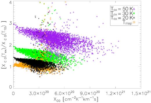
Xco factor distribution comparison (derived as described in Section 7.1), y axis is in the form Xco(Tex)/Xco(T10), where the excitation temperature |$\mathrm{T_{\mathrm{ex}}}$| is equal to 20, 30, and 50 K, respectively (T10 is for Tex = 10K), T10 median value is |$2.2\times 10^{20}\,\mathrm{cm}^{-2}\, \mathrm{K}^{-1}\, \mathrm{km}^{-1}\, \mathrm{s}$|. Tmap means that column density calculation was based on the pixel-by-pixel Tex map (Fig. 10), derived for each line of sight from the 12CO peak emission.
In Fig. 18 we plotted the angular distribution of Xco for Tex = Tmap, the median value is |$2.2\times 10^{20}\,\mathrm{cm}^{-2}\, \mathrm{K}^{-1}\, \mathrm{km}^{-1}\, \mathrm{s}$|. Small scale (compared to cloud extension) Xco variations are present in almost all the cloud, up to a factor of 2. In general, there is no direct relation between Xco and integrated intensity (Fig. 4). An exception is in [C2], [D2], and [E2], where there are evidences of an inverse proportion between Xco and 12CO integrated intensity. This is not unexpected since 12CO self-absorption in these regions (see last part of Section 5.1).
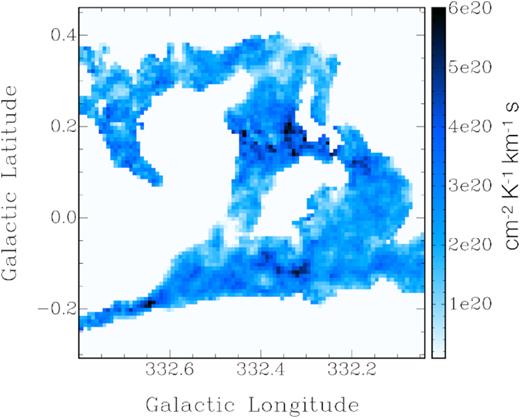
Xco factor local variation map derived from the ratio between the 12CO integrated intensity and the N(H2) computed from 13CO for a Tex derived from the 12CO peak temperature map.
In Fig. 19 is illustrated the corresponding histogram, showing that the values are mostly (|${\sim }80{{\ \rm per\ cent}}$|) in the range between 1.7 × 10²⁰ and |$3.5\times 10^{20}\,\mathrm{cm}^{-2}\, \mathrm{K}^{-1}\, \mathrm{km}^{-1}\, \mathrm{s}$|.
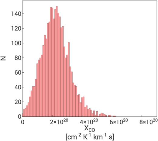
Histogram of the Xco distribution derived from a Tex computed from 12CO peak emission map as in Fig. 18. The median value is |${\approx }2.2\times 10^{20}\,\mathrm{cm}^{-2}\, \mathrm{K}^{-1}\, \mathrm{km}^{-1}\, \mathrm{s}$|.
A deeper discussion on Xco variation across the ring molecular cloud is presented in Section 10.3.
7.2 X|$\mathrm{_{CI}^{809}}$| factor
The linear fit m · FCI, being FCI the [C i] integrated intensity in |$\rm \, K\, km\, s^{-1}$|, gives for X|$\mathrm{_{CI}^{809}}$| the values of (1.77 ± 0.03) × 1021, (1.83 ± 0.02) × 1021, and |$(1.97\pm 0.02)\times 10^{21}\,\mathrm{cm}^{-2}\, \mathrm{K}^{-1}\, \mathrm{km}^{-1}\, \mathrm{s}$|, respectively, for N(H2) traced by 12CO, 13CO without adding dark gas and 13CO adding the dark gas fraction.
We report the value of |$X_{\mathrm{CI}}=1.10\times 10^{21}\,\mathrm{cm}^{-2}\, \mathrm{K}^{-1}\, \mathrm{km}^{-1}\, \mathrm{s}$| by Offner et al. (2014) and |$X_{\mathrm{CI}}=1.01\times 10^{21}\,\mathrm{cm}^{-2}\, \mathrm{K}^{-1}\, \mathrm{km}^{-1}\, \mathrm{s}$| obtained from the numerical simulation of Glover et al. (2015) that were derived for the CI emission at 609 μm, about half of the value we derive from the data.
8 CO AND [C i] LINE RATIOS
8.1 evans plot
In the following, we present ratios between the 12CO, 13CO, and [C i] lines using a signal-to-noise (SNR) visual discriminator type of graph known as an evans17 plot, where high SNR pixels are more evident than lower ones. Here we give a brief description on how to read evans plot taking as reference Fig. 20 (see also Burton et al. 2015). Each plot consists of two pictures, one showing data (left-hand panel) and one showing a Hue Vs Saturation colour table (right-hand panel). Each pixel in the data map has hue and saturation values, which are codified into SNR and data values (the ratio value in this case) using the colour table, according to the axes scales. In this way, those pixels with high SNR values are more evident with respect to lower SNR pixels, which fade into grey independently from their ratio value, giving them a lower visual weight.
evans plot of the 12CO/13CO integrated intensity map over the ring VLSR range. Left-hand panel – Each pixel in the ratio map possesses hue and saturation values that are decoded to SNR and ratio values using the colour table on the right-hand panel (see 8.1 for details on evans plot). In white is the contour representing 13CO integrated emission at |$3\rm \, K\, km\, s^{-1}$|.
8.2 12CO/13CO ratio
In Fig. 20 is shown the ratio between integrated intensity map of 12CO and 13CO, over the ring spectral channel range. Each zeroth moment map was derived applying the same 13CO 3D mask to both datacubes. The ratio exhibits almost everywhere a value >1, increasing towards the cloud edge respect to innermost regions, in which it assumes values in the range [2–4]. A small region located in [D2], around (ℓ, b) = (332.3°, 0.2°), shows a ratio <1; this could be explained by 12CO self-absorption (Fig. 7).
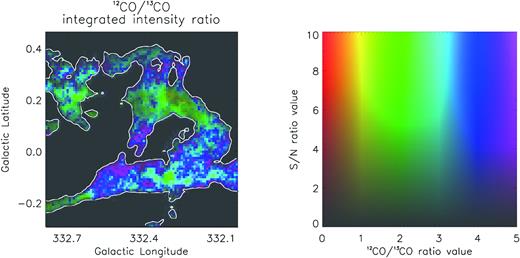
8.3 [C i]/13CO ratio
The C abundance is expected to increase in the external layers of GMCs where the FUV radiation dissociates the CO, so that the [CI]/CO ratio may be greater than in the innermost parts of the cloud. To investigate the [CI]/13CO in the ring we regrid the 13CO cube to the [C i] coarser resolution and applied to both the same [C i] 3D mask. In Fig. 21 we present the integrated intensity maps ratio between [C i] and 13CO.
![evans plot of the integrated intensity map [CI]/13CO ratio along the ring VLSR velocity range. White contour is 13CO integrated intensity at $2\rm \, K\, km\, s^{-1}$.](https://oup.silverchair-cdn.com/oup/backfile/Content_public/Journal/mnras/484/2/10.1093_mnras_sty3510/1/m_sty3510fig21.jpeg?Expires=1749926495&Signature=Sr3qYhr6rNLHDBl7sCTJktwiFzmS-yzGBoSgG9Ry~J-2YLH12IYjO036dPx8dMiuqfRdgHuzJaezGfE3~sR9nJ9fKud5T8DNohaRfGQollfQ7rbjrFpMdYycaUe1fwz-5xtoaGSt9uHZ6HpAnYDyfXVolLfHCwhyX~~Bk4A42lkNJz8ggsyDxzFZvl~lGNwmGXViMy-7CNpKh5FB7wkcK0uDsHY2snxjjTbs7Y~A5kWnFlz-gkOcaH4sXnvv-ou7LDIObOk6hyhdM9Qtl35r26a35MymnPr9ArfGpAH2ihIne6uhJ5WA6K3KaIA-lyax0dTjohqmtwERxN~zyZk5ig__&Key-Pair-Id=APKAIE5G5CRDK6RD3PGA)
evans plot of the integrated intensity map [CI]/13CO ratio along the ring VLSR velocity range. White contour is 13CO integrated intensity at |$2\rm \, K\, km\, s^{-1}$|.
The ratio between the zeroth moment maps possess values <1 along almost all the lines of sight passing through the thickest region of the molecular ring, with lower peaks in [NW-R] and [N-R]. Ratio values are >1 at the edge of the cloud subregions [SE-R], [SW-R], [C-R], and [N-R], although here 13CO detection drastically decreases, lowering the signal-to-noise level and making pixels less distinguishable. Interestingly, some sections of the ring edge have a ratio <1, in [NW-R], in eastern [C2] and around (ℓ, b) = (332.25°, 0.0°).
To better characterize the ratio values dispersion, we explore the ratio voxels distribution along the ring velocity range considering only those included in the 3D [C i] mask (see Fig. 22, 2D heatmap scatter plot between 13CO and [CI]/13CO). The median of the ratio for the whole cloud is equal to 0.5, and its tendency is to decrease with the increase of 13CO emission, following a |$y_0 +\frac{a}{x-x_0}$| law, with a = 0.43 ± 5.2 × 10⁻³, y0 = 0.27 ± 3.8 × 10−3 and x0 = (8 ± 1) × 10−3. There are few ratio >1 voxels that come from low 13CO emission, the analysis of their position with respect to the molecular ring confirms that all of them are at the edge of the CO molecular ring.
![2D heat map between 13CO datacube regridded to [C i] resolution and [CI]/13CO voxels. The black line represents the fit in form: $y_0+\frac{a}{x-x_0}$ (parameters are reported in Section 8.3).](https://oup.silverchair-cdn.com/oup/backfile/Content_public/Journal/mnras/484/2/10.1093_mnras_sty3510/1/m_sty3510fig22.jpeg?Expires=1749926495&Signature=VvOjCACh73w1CY71yStr2b7pVqO82fZ~UX9lE8QiFN0sIbctBLYazGN84ruq2mYBGY2Cy3JDCXpb-xSatsKVl14uHllP18~Z2ronsw26SodJnhm4FrIefa57UuxB~5TC08KVNnKDvz0DxIoFNa2MWxKYBOmCame~RxQRGTU3gLasFoihNlvqkT7P~Ob0CdjyF05qFjxqCxgvSdozBmEKh6PdhczqAdtNQbcV1bPohbvCcOX8wkp-8HeVyac7~85UunUIj4FKnJGootRJiRoqtYI5vJ43zzvT3-ZbOSkmWbbSFS3OpgEFQ7AIwFpcdvIJxIisMnn-yxeGaUvlShcZBg__&Key-Pair-Id=APKAIE5G5CRDK6RD3PGA)
2D heat map between 13CO datacube regridded to [C i] resolution and [CI]/13CO voxels. The black line represents the fit in form: |$y_0+\frac{a}{x-x_0}$| (parameters are reported in Section 8.3).
9 C18O CLUMPS CLASSIFICATION
Since C18O emission is generally weak, due to the low isotopic abundance ratio compared to 12CO and 13CO, its detection is mostly likely to be optically thin. This makes the C18O line a probe through the entire molecular clouds column, sensitive in particular to the highest column density regions, when 13CO (and even more so 12CO), is optically thick. In order to investigate the highest column density clumps within the molecular ring, we decomposed it applying the clumpfind algorithm (Williams, de Geus & Blitz 1994) to the C18O emission cube, binned and smoothed in the same way as in moment maps computation (see Section 5.1). We limited our analysis to the ring velocity range; however an expansion of this work, performed on 10° of the Galactic Plane binned C18O datacube, is presented in Braiding et al. (2018). After a series of tests we selected the value of 0.35 K, equivalent to 3.5σ, for both input parameters inc and low. We set a threshold of 10 voxels on the minimum voxel number for a clump to be detected. We verified for false detection comparing C18O and 13CO spectral lines passing through each clump centroid. To avoid false detection of a single clump as two distinct clumps we set a minimum centroid distance equal to seven voxels; all the clumps passed this verification step. The final detections are summarized in Table A1 with their physical characteristics.
The resulting total virial mass is |$\mathrm{M^{tot}_{vir}}=4.9\times 10^4\,\mathrm{ M}_{\odot}$|. In order to compare it to the total mass derived under LTE assumption |$(\mathrm{M^{20}_{LTE}}$|) we applied the method described in Section 6 including only voxels belonging to a clump related to the ring. According to the different Tex used, the total LTE clump mass traced by C18O is 0.8 × 10⁵, 1.1 × 10⁵, and 1.5 × 10⁵ M⊙, respectively, for Tex = 10, 20, and 30 K. These values are similar to the LTE masses calculated for voxels included in the 3D smooth mask (Table 4). Comparing the total mass of the C18O clumps and the total mass of the ring derived from 13CO, under the LTE assumption and taking the same Tex for both tracers, the fraction of gas in C18O clumps is 59 and |$76{{\ \rm per\ cent}}$|, respectively, for Tex = 10 and 30 K. Changing inc and low parameters in clumpfind, from 0.35 to 0.4 or 0.3 K, respectively, decreases or increases the LTE mass by |${\sim }20{{\ \rm per\ cent}}$| for all Tex, as a consequence of smaller or bigger clumps being identified by the algorithm.
We note that the clumpfind algorithm found four clumps that are in a portion of the sky in which the C18O integrated intensity has values equal to zero. This discrepancy is due to the C18O 3D mask process creation. As described in Section 5.1, the 3D mask is derived from the smoothed cube. This operation decreases the intensity level of a weak emission extended for few voxels. As a consequence, this emission could result below the sigma threshold set on the smoothed cube in order to define the 3D mask extension. These off mask clumps are indicated with A, B, C, and D in Fig. 23 and, respectively, correspond to GMCC332.50+0.32, GMCC332.39+0.35, GMCC332.42+0.02, and GMCC332.29-0.01 in Table A1. Because of the exclusion from the 3D mask, the mass of these clumps is not present in the N(H2) derivation as in Section 6 and reported in Table 4. Assuming a Tex = |$20\rm \, K$| their total mass results to be 104 M⊙, equal to |${\sim }8{{\ \rm per\ cent}}$| of the total C18O clump mass.
![Plot of Hi-GAL compact sources (see Section 10.2) with a near distance solution between [3,4] kpc (red) and C18O clump ellipsoids as reported in Table A1 (green). The black spline is the path along which are plotted the Hi-Gal dust clumps properties as in Fig. 27.](https://oup.silverchair-cdn.com/oup/backfile/Content_public/Journal/mnras/484/2/10.1093_mnras_sty3510/1/m_sty3510fig23.jpeg?Expires=1749926495&Signature=IJMr8DnI7vKQ8zXor1Oh5uyzFX6a66tYTm7CMxfNmKpF9C6mJuLht3LcD6cChR~~SEZrRDGPqZgdsA3~rA0ND7PecMEAMyaucRdrsMl6-K5bEJ1kLgP2uNOT0BQcJmvo9qDBOh3LrQxPAdhgxhDnbCsy7IwgoDROpeYmMX68amUFJ8QlogtPZzVro1vG6cJLD0f66uREGZFwMf4w91uXR6GBZ8FSBCUg7NbMHpveN8ReauMzj5pkr8vschVkMcLfzsBkU72mnzFA0c2gX9W~ULbGoMsoWvHgAA76Nu0-nyNdwAyl2PC-Ua9ErCS8EQREu1NX0M5vU4vr1FkEEf4Iwg__&Key-Pair-Id=APKAIE5G5CRDK6RD3PGA)
The virial parameter, defined as |$\mathrm{\alpha _{vir}}=\mathrm{M_{vir}/M^{20}_{LTE}}$| and plotted in the Table A1 (column 11), gives an indication about the dynamical state of each clumps. Typical values are in the range [0.2–0.4] suggesting that they are not being supported against gravitational collapse. Though care is needed in this interpretation since masses derived under LTE assumptions applied depend on the Tex and C18O abundance ratio choice.
10 DISCUSSION
In the following sections we will describe a method, based on the 13CO emission, to separate dust emission across the Galactic spiral arms, giving an estimate of the total mass traced by dust through the ring region. We will also discuss the different physical conditions in the cloud and how these suggest a scenario in which the molecular structure shows different evolutionary stages: quiescent clouds in which star formation is occurring at its earliest stage or not yet initiated, and active clouds in which star formation is ongoing at a later stage. In doing so, we will compare the C18O with Hi-Gal clumps associated with the G332 ring cloud.
10.1 Dust across the Galaxy
As discussed in Section 6.5, the overall N(H2) derived from the dust emission is the sum of all contributions along the line of sight. To compare it to N(H2) traced by the 13CO we first consider Fig. 14, relating dust column to 13CO line flux. There are two sets of point here, one (group A) showing a linear correlation, the other (B) not. The former demonstrates the link between flux and column density for most regions, which we now decompose into contributions coming from separate spiral arms along the line of sight.
We note that in the N(H2) column density traced by dust (Fig. 13, which comprises all infrared emission from this region) it is possible to find, to first approximation, a coherency between the dust and 13CO and 12CO integrated flux (Fig. 4). In particular, as shown in Fig. 13, in [SE-R] and [SW-R] 13CO integrated flux peaks are close to dust column peaks. The West side of the ring, [W-R], and part of [NW-R], present low integrated CO emission while the dust is bright. Bright dust, in general, follows the ring, a likely consequence of it arising from the region too. However, focusing on the ring CO and dust emission, we need to separate dust related to different Galactic spiral arms. In the following we describe our approach.
According to the average CO spectral line profile and following the spiral arm scheme adopted in this paper (Fig. 5), we separated the 13CO emission into four velocity ranges (R1, R2, R3, and R4), choosing the near or far solution coherently with any H i emission local minimum (see Fig. 3):
R1: [−115 to |$-75\rm \, km\, s^{-1}$|] [intra-arm Perseus/Norma far]
R2: [−74 to |$-56\rm \, km\, s^{-1}$|] [Norma far]
R3: [−55 to |$-44\rm \, km\, s^{-1}$|] [Scutum-Crux near] (ring)
R4: [−44 to |$-30\rm \, km\, s^{-1}$|] [Scutum-Crux near]
This scheme follows the position velocity (PV) plot of Fig. 6. We excluded 13CO emission coming from −30 to |$+10\rm \, km\, s^{-1}$| since it is localized in small structures and its integrated intensity is negligible with respect to other velocity intervals. To separate the dust emission coming from each of the spiral arms we computed, following the method of Section 5.2, for each velocity interval, a 13CO pixel-by-pixel moment zero map normalized to the total integrated intensity relative to the VLSR interval [|$-115,-30\rm \, km\, s^{-1}$|] (see Fig. 24), each of which is subsequently multiplied by the N(H2) derived from dust SED fit (Fig. 13). In this way we created four different N(H2) dust maps (see Fig. 25 one for each spiral arm). Our approach is based on two assumptions that N(H2) traced by 13CO is proportional to 13CO integrated intensity and that the emission from dust coming from regions where there is no CO emission is negligible (see below for H i contributions). Thus, we are able to compare a directly measured quantity (13CO emission) to N(H2) dust. We also excluded the molecular hydrogen not traced by CO in this analysis.
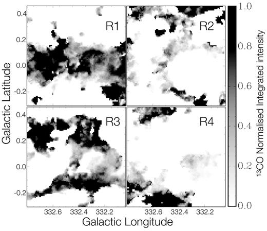
Normalized 13CO integrated intensity map belonging to the defined velocity ranges as in Section 10.1. Each pixel represents the multiplication factor applied to the corresponding pixel in the dust derived N(H2) map; thus it is possible to obtain a fractional molecular hydrogen column density traced by dust for each velocity range.

Scatter plots, between 13CO integrated intensity and N(H2) dust for each spiral arm, are shown in Fig. 26. Higher column densities belong to [R1] and [R3]. In each plot we use different colours for those pixels having a normalized 13CO integrated intensity map equal to 1, while the other pixels are in grey. Both of them follow a direct proportional relation but have not the same offset: grey points starts at zero while coloured pixels begins at about 1022 cm−2 for all the ranges. Pixels belonging to the offset group comes from regions in which the normalized 13CO moment zero map has values equal to 1, which means the total 13CO integrated intensity (along the whole line of sight) has contributions coming from a single velocity interval only, without contamination from other clouds at different distances. These are those pixels in black (value equal to 1) in the normalized moment zero maps (Fig. 24); for them dust emission can be constrained in a specific velocity range since there is no other CO detection on the same line of sight.
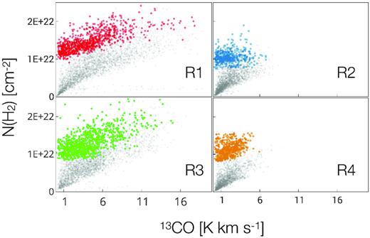
Scatter plots between normalized moment zero 13CO (x axis) and fractional N(H2) dust relative to all velocity intervals (as defined in Section 10.1). For each scatter plot we use colours for those pixels whose normalized 13CO integrated intensity map is equal to 1 (see Fig. 24). The grey points represent all the other pixels.
In Table 6 are reported linear fit parameters for each velocity interval, considering only coloured points as in Fig. 26. The offset value is almost the same for every range, around 1022 cm−2, this value is similar to the mean H2 column density traced by dust in regions where no CO emission is detected along the whole Galactic velocity range (considering the 12CO integrated intensity map in the [|$-110, +10\rm \, km\, s^{-1}$|] VLSR range). This could be a consequence of the infrared background emission coming from this part of the sky, [R1] shows the largest background having the largest velocity width. The fit parameters (except for [R2], but this has the lowest contribution to the total emission), are comparable to the fit parameters reported in Fig. 14. The relative contributions of each velocity range with respect to total 13CO integrated intensity, along the whole line of sight, are 35, 8, 47, and 10 per cent, respectively, for R1, R2, R3, and R4. Although, R3 is only |$10\rm \, km\, s^{-1}$| wide, it accounts for almost half of the total 13CO emission in G332.
Linear fit parameters for each velocity interval from plots in Fig. 26 derived using the unity value pixels in the normalized moment zero maps (coloured pixels). Numbers between parenthesis are interval widths.
| Fit parameters | ||
|---|---|---|
| N(H2)dust = m · F13CO + b | ||
| Interval | m | b |
| |$(\rm \, km\, s^{-1})$| | |$\mathrm{(cm^{-2}\,K^{-1}\, km^{-1}\, s)}$| | (cm−2) |
| R1 (40) | 6.1 × 10²⁰ ± 0.2 × 10²⁰ | 1.21 × 10²² ± 1.0 × 10²⁰ |
| R2 (18) | 1.3 × 10²⁰ ± 0.6 × 10²⁰ | 1.03 × 10²² ± 1.3 × 10²⁰ |
| R3 (11) | 7.4 × 10²⁰ ± 0.3 × 10²⁰ | 1.01 × 10²² ± 1.5 × 10²⁰ |
| R4 (14) | 6.1 × 10²⁰ ± 0.7 × 10²⁰ | 1.02 × 10²² ± 1.5 × 10²⁰ |
Taking into account a near or a far distance solution, the mass traced by the disentangled dust in each velocity interval is reported in Table 7, together with the mean neutral hydrogen column density, N(HI), which is the |$13,$||$13,$||$6,$| and |$8{{\ \rm per\ cent}}$| of N(H2) column density (derived from dust) in [R1], [R2], [R3], and [R4], respectively.
Summary table of the four velocity ranges in which is divided the dust emission of the G332 Galactic plane sector. The mean N(H2) is traced from the fractional dust emission as described in the Section 10.1. The distance is computed from the VLSR value of the centroid velocity of each interval.
| Interval | Distance | Mass | Mean N(HI) | Mean N(H2) |
|---|---|---|---|---|
| kpc | M⊙ | 1020 cm−2 | 1020 cm−2 | |
| R1 | 8.8 | 12.2 × 10⁵ | 13.0 | 100 |
| R2 | 10.5 | 6.6 × 10⁵ | 6.9 | 54 |
| R3 | 3.7 | 2.00 × 10⁵ | 6.1 | 95 |
| R4 | 2.9 | 0.5 × 10⁵ | 4.6 | 56 |
| Interval | Distance | Mass | Mean N(HI) | Mean N(H2) |
|---|---|---|---|---|
| kpc | M⊙ | 1020 cm−2 | 1020 cm−2 | |
| R1 | 8.8 | 12.2 × 10⁵ | 13.0 | 100 |
| R2 | 10.5 | 6.6 × 10⁵ | 6.9 | 54 |
| R3 | 3.7 | 2.00 × 10⁵ | 6.1 | 95 |
| R4 | 2.9 | 0.5 × 10⁵ | 4.6 | 56 |
Comparing HI and CO column densities, across the −110 <VLSR|$\lt +10\rm \, km\, s^{-1}$| velocity range, we found that the amount of atomic gas is about |${\sim }10{{\ \rm per\ cent}}$| of the column density of the molecular gas, so that the dust column density is dominated by emission from dust within molecular clouds. The total mass traced by dust across the whole sky portion defined by the ring region in the Galaxy velocity range (−110 <VLSR|$\lt +10\rm \, km\, s^{-1}$|) is ∼2.15 × 10⁶ M⊙.
10.2 Star formation activity along the molecular ring
The overview image in Fig. 1 shows the Southern side of the ring hosting several signposts of star formation with activity (masers and H ii regions) counterpoised a less active Northern side. In order to investigate this difference we compared the C18O clumps distribution (reported in Table A1) to the compact sources distribution taken from the Hi-GAL catalogue (Elia et al. 2017) classified for different stages of star evolution.
The Hi-GAL sources (hereafter called dust clumps) selected for our analysis have coordinates that fall inside the C18O clumps ellipsoid extension (with semi-axis defined by Δℓ and Δb FWHMs derived by clumpfind), and a near distance solution between 3 and 4 kpc. In order to avoid the exclusion of sources not satisfying these criterion, but potentially linked to the molecular ring, we included all the dust clumps that totally (or partially) fall in the portion of sky covered by the angular extension of the C18O integrated intensity map (see Fig. 23). The total mass of all the dust clumps considered is ≈6.8 × 10⁴ M⊙, equal to the |$35{{\ \rm per\ cent}}$| of the ring mass traced by 13CO at Tex = |$30\rm \, K$|.
The Lbol/Mclump ratio is a useful indicator of the star formation activity ongoing in the hosting clump (Molinari et al. 2008; Elia & Pezzuto 2016). In order to examine the star formation activity along the molecular ring, in Fig. 27 we plot the Lbol/Mclump and Tclump values of the dust clumps following the path defined from the [E,SE-R] to the northern part of [C-R] (see Fig. 23).
![Plot of Hi-Gal Tclump (left-hand panel) and of ln[Lbol/Mclump] (right-hand panel) ratio derived from the bolometric luminosity of the clump and its mass (in M⊙). The x axis is the offset distance from the initial point of the path (at coordinates ℓ ∼ 332.75° and b ∼ −0.25°) defined in Fig. 23 by the black spline.](https://oup.silverchair-cdn.com/oup/backfile/Content_public/Journal/mnras/484/2/10.1093_mnras_sty3510/1/m_sty3510fig27.jpeg?Expires=1749926495&Signature=o0-0cKMWTv0yFLbnfj~ZcdMcVTHXncILhAbDuu5hs1Q1id1kcMeNbZSBcmBmyNCf9RZREtS2jr2d3Xnl2mAfYNNP0XqhvuQ3qPrz5rabkbbCm9zf9wRPSndLGUS8C3wgRpbOdHWvFZYTAm5TaAXpL07cTrhQ7eKyBHDSjogav9E7gNsx1wx2ufP1-O-6gt-f7QNXyfosEOz3VDqt6gvmlMjwJZdbzz~xMSo3QHDtkkKPfadvCLZc7GsIGwBBewEgMfH1MqSLt2DhYmfRn-KC60ZPzgj-guSHpd8hRtCC3atz-M7gFz5zZTdAHdH6Ewk7-Q~WgAE2lg~GIf4pzqD5pQ__&Key-Pair-Id=APKAIE5G5CRDK6RD3PGA)
Plot of Hi-Gal Tclump (left-hand panel) and of ln[Lbol/Mclump] (right-hand panel) ratio derived from the bolometric luminosity of the clump and its mass (in M⊙). The x axis is the offset distance from the initial point of the path (at coordinates ℓ ∼ 332.75° and b ∼ −0.25°) defined in Fig. 23 by the black spline.
The highest dust clump temperatures are in the Southern ring, as well as the highest Lbol/Mclump ratios, both decrease following the path. The C18O clumps corresponding to the Southern ring (as reported in Table A1) exhibit in mean, higher values in 13CO, C18O average temperatures and in velocity dispersion, while those relative to the Northern cloud show lower values for the same quantities. These factors suggest a difference in the star formation activity along the cloud: the dust cores in the Southern ring exhibits (on average) hotter temperatures suggesting that star formation activity is going on, while the Northern cores, colder, indicate that the star formation has not yet started, or at an earlier stage.
10.3 Local Xco variation
12CO (J = 1 → 0) emission is often used in the determination of the N(H2), and total molecular mass, through the use of the Xco factor, especially for extra-Galactic sources. Thus, it is important to understand how the physical conditions of the emitting gas contribute to any variation in the X factor. Considering the cloud distance and the pixel dimension of 30 arcsec we are able to examine Xco variations on parsec scales (at |${\sim }0.5\rm \, pc$|).
The approach of our Xco analysis uses equation (7), where N(H2) is traced by 13CO under different Tex assumptions, or N(H2) traced by dust. As shown in Section 7.1, the average Xco is found to increase with the assumed Tex used to derive the column density.
A pixel-by-pixel map of the cloud Xco values is shown in Fig. 18, the highest values are in [NW-R], and in part of [N-R] (at b ∼ 0.2° and 332.45° < ℓ < 332.15°), in [A6], in [B6], and around the position (ℓ, b) = (332.3°, −0.1°) of typically |${\sim }5\times 10^{20}\,\mathrm{cm}^{-2}\, \mathrm{K}^{-1}\, \mathrm{km}^{-1}\, \mathrm{s}$|.
12CO spectral lines, where the Xco is higher, show lower 12CO intensity compared to ring average, as does 13CO as well, and in general present a non-Gaussian spectrum profile. In many cases, 12CO is self-absorbed, while 13CO and C18O peak at the 12CO local minimum (as shown in Fig. 7).
Local decrease in intensity of the 12CO/13CO ratio (Fig. 20) corresponds to higher Xco factor (Fig. 18), where the 12CO/13CO ratio is lowest, the CO is most optically thick and the Xco is highest.
This is not unexpected since, by definition, our Xco map derives from the ratio between N(H2) traced by 13CO (proportional to 13CO integrated intensity through the optical depth integration; see equations 4 and 5) and 12CO integrated intensity. These optically thickest regions show significant decrease in 12CO emission with respect to 13CO.
10.3.1 Xco and Tex
To further investigate the physical conditions underlying the observed Xco distribution (Fig. 19), we looked at the variation of Tex around the molecular ring. In Fig. 28 are shown the scatter plots of Tex versus Xco for each sub-region of the cloud. The Tex value was derived from the 12CO peak temperature for each sight line, while the Xco was computed by using the N(H2) traced by 13CO, assuming in the 13CO column density a Tex derived from the dust temperature computed by the SED fit (see Section 6.5). In Table 8 are summarized the Xco and Tex mean values for each region.
![Xco factor plots for each ring sub-region as per Fig. 1. The range of x and y axes are the same for each plot. The plot [SE-R] comprises only pixels coming from [SE-R], excluding those with ℓ > 332.65°, which are reported in the sub-plot indicated with [E,SE-R] (Eastern-South East, Region).](https://oup.silverchair-cdn.com/oup/backfile/Content_public/Journal/mnras/484/2/10.1093_mnras_sty3510/1/m_sty3510fig28.jpeg?Expires=1749926495&Signature=no3H2iJn9FrWNFC6Pv6X5tCMB4vpxOf0mVqfgoz4gplAL57hsJuBRX-vNInUFiwY-QB4caBRLpyuBn-mQNAhowHZH6~SYNuTtq2r7Sv4wVDf6mn7rv91L2mMUX3qsDtqXWIlMyz5tE8nULmxkA6Xya9-gtlRhzANnp~oFKOFem5AdEzLCCd6RBHHRbbdxjaFBCAJ8inBDYHFLE~wL7B-oPVmWIbht0GW5mBYrpwO9sYgjUHpVq57qCS4Xq-d40WOXQKKwZq2~xJC7TIfgzUZfWcDdXVAeSR-pCq60oK86XlDBIFKWRMWX8KPytLLESej4cnpxCVIwh2Xh0xMANO0pA__&Key-Pair-Id=APKAIE5G5CRDK6RD3PGA)
Xco factor plots for each ring sub-region as per Fig. 1. The range of x and y axes are the same for each plot. The plot [SE-R] comprises only pixels coming from [SE-R], excluding those with ℓ > 332.65°, which are reported in the sub-plot indicated with [E,SE-R] (Eastern-South East, Region).
Summary table of mean Xco, Tex, and mean [CI]/13CO ratio values per region in Fig. 28. The mean value for the Tex is derived from the mean peak emission of the 12CO along the line of sight of each region.
| Region | Mean Tex | Mean Xco | [CI]/13CO |
|---|---|---|---|
| K | |$\mathrm{cm}^{-2}\, \mathrm{K}^{-1}\, \mathrm{km}^{-1}\, \mathrm{s}$| | ||
| [N-R] | 14 | 2.6 × 10²⁰ | 0.7 |
| [NW-R] | 15 | 3.8 × 10²⁰ | 0.5 |
| [W-R] | 16 | 2.5 × 10²⁰ | 0.5 |
| [SW-R] | 18 | 2.6 × 10²⁰ | 0.6 |
| [SE-R] | 21 | 2.4 × 10²⁰ | 0.6 |
| [E, SE-R] | 15 | 3.3 × 10²⁰ | 0.4 |
| [C-R] | 17 | 2.1 × 10²⁰ | 0.7 |
Examining Fig. 28 we note a general decrease in the dispersion of Xco values, moving from [N-R] towards [SE-R], while Tex increases. This behaviour in Tex is similar to the temperatures and Lbol/Mclump ratio trend observed in the dust clumps (Fig. 23) and is consistent with a stellar evolution gradient scenario: the Southern cloud hosts active and more evolved star formation sites, which heat the surrounding gas so increasing its temperature. On the contrary, the Northern cloud hosts less and, on average, earlier stage star formation sites, the gas is colder compared to the South and the peak emissions are the lowest, as well as the velocity dispersion and the column densities.
Supporting a scenario in which the Southern cloud is more active than the Northern, as illustrated in Fig. 1, the literature reports many indicators of star formation activity, as H ii regions (see Section 5.2) and masers, localized in the Southern ring: 6 GHz methanol maser (Caswell et al. 2010), water maser (Walsh et al. 2014), class I methanol maser at 36 and 49 GHz (Voronkov et al. 2014), and 95 GHz maser (Yang et al. 2017).
Recently Kong et al. (2015) reported for the California Molecular Cloud high Xco values dispersion for cold quiescent regions and an inverse correlation between Xco and Tex. They argued that this correlation could explain the range of Xco values, found for different GMCs, as a consequence of the different amount of warm gas heated by OB stars in the cloud. The G332 molecular cloud presents similar behaviour, where the coldest parts of the cloud show the most scattering and highest Xco values and the lowest Tex, while the most active regions show the opposite behaviour.
10.4 [C i]
The UV radiation coming from the massive young stars photodissociates the surrounding gas, creating a PhotoDissociation Region (PDR), where the carbon is mainly in atomic form, in neutral or singly ionized state (Tielens & Hollenbach 1985; van Dishoeck & Black 1988); similarly, the external layer of molecular clouds are exposed to the diffuse far-UV radiation, photodissociating the CO before it reaches a column density high enough to enable self-shielding. To inspect the atomic carbon distribution around the cloud, in Fig. 21 is illustrated the ratio between the integrated intensities of [C i] and 13CO. As expected, the outskirts of the clouds possess the highest ratio values, though with the lowest SNR. Interestingly, [NW-R] and [W-R] present an exception: low ratio values at the edge facing the North–West direction, while the edge towards South–East presents higher values. Looking at the sightlines passing through the innermost part of the cloud, the regions with the lowest [CI]/13CO ratio values are [N-R], [NW-R], [E,SE-R], and part of [W-R]. Profiles showing the ratio as a function of velocity are in Fig. 29. They were derived from the [C i] and 13CO (regridded to the [C i] resolution) datacubes, both masked using the same [C i] 3D mask, the resulting profiles were then plotted applying a Hanning smooth of order 3. The resulting picture is of a northern ring, [N-R] and [NW-R], with mean ratio values of 0.3 centred at VLSR = |$-50\rm \, km\, s^{-1}$| (we consider the second peak at VLSR = |$-42\rm \, km\, s^{-1}$| belonging to another cloud; see Fig. 3), while the southern ring has a mean ratio value of 0.5, peaking at 0.6 in the external layer of the cloud. In [SW-R] (aperture D) the mean ratio spectral profile shows a constant value going deeper in the cloud, a possible indication of photodissociation in the cloud interior caused by star formation activity. Apertures A and C, belonging to the southern cloud, show a small dip in the innermost part of the ring, where the 13CO emission increases. Regarding aperture E, we note that the emission velocity centroids of the [C i] and the 13CO emissions are close to VLSR = |$-50\rm \, km\, s^{-1}$| (Fig. 8), while we consider the second peak at VLSR = |$-42\rm \, km\, s^{-1}$| belonging to another cloud.
![Plots of the mean spectral profiles of [CI]/13CO ratio right for the different apertures indicated with different letters in the left-hand image. The image map represents the 13CO integrated intensity map, with the green contours its extent.](https://oup.silverchair-cdn.com/oup/backfile/Content_public/Journal/mnras/484/2/10.1093_mnras_sty3510/1/m_sty3510fig29.jpeg?Expires=1749926495&Signature=c4akyf4ZkQPBkMNE3R5BH2SWcl6eAIePpOcbPzqvVHhAPSxYmH9FC1q-6u8l3la3YKb~K1zZWoGBkyIEYEf77H9Hpbos0jCd23YW7k0PkFrGoT-24dnnhIe5EB1mXOGb8CzMXd4qIXmXKhBR9splgcjR8KW59MZk8Y5P1In3B5B-TShTRabdaMOYpA7SvcT84flaRDaNIzdfvcgq9rVldZBytDQmmqIODxqhhq1kq-aqwQ~l1dsNEBizRep-FjXYGX3CEgA~AJsbf41XHfvAu5wfUs4WkX6ACB3jG2cXSShZlpHL1WWeSS9~WbF7kQEgNhdEETvx3B40ltkXERHRXQ__&Key-Pair-Id=APKAIE5G5CRDK6RD3PGA)
Plots of the mean spectral profiles of [CI]/13CO ratio right for the different apertures indicated with different letters in the left-hand image. The image map represents the 13CO integrated intensity map, with the green contours its extent.
We conclude that the fraction of atomic carbon, with respect to its molecular form, is lower in the Northern cloud than in the Southern cloud. The latter possesses the highest photodissociation levels due to increased radiation fields. We speculate that [NW-R] is the most quiescent part of the cloud, and the difference between North and South is driven by a star formation activity ongoing at a later stage in [SW-R] and [SE-R], compared to [N-R], [NW-R], and [E,SE-R]. This further strengthens the hypothesis of a difference in the star formation activity between northern and southern ring.
10.5 CO and 8 |$\mu$|m emission
IRDCs are regions in which the gas is cold and dense, absorbing background IR emission. They provide suitable targets to look for signposts of early star formation activity (Teyssier, Hennebelle & Pérault 2002; Rathborne, Jackson & Simon 2006; Simon et al. 2006). The dust temperature map reported in Fig. 11 suggests that the North–Western ring is the coldest region, thus it is likely to host IRDCs. In Fig. 30 we plot the angular positions and equivalent radius size of the IRDCs (red circles) identified by Peretto et al. (2016), overlaid on the Xco map. Despite the coarser angular resolution of the Xco, compared to the 16 arcsec Hi-GAL maps, it is possible to see a spatial correlation between their positions and the angular extent of the molecular cloud.

In Fig. 31 is shown the Spitzer|$8\,\hbox{$\mu $m}$| image, in green contour is the angular extension of the 13CO integrated intensity map, while the red contours represents the dust temperature as per Fig. 11. We note that the distribution of cores with lowest dust temperatures precisely follow the extinction features seen in |$8\,\hbox{$\mu $m}$|. Moreover, between 332.3° < ℓ < 332.1° and −0.1° < b < 0.3°, an arc-like extinction feature is clearly seen, following the CO emission in the sky portion defined by northern [SW-R], [W-R], and [NW-R] and southern [N-R]. The same correspondence between lowest dust temperatures values and |$8\,\hbox{$\mu $m}$| extinction is seen in [E,SE-R]. On the other hand, the highest dust temperatures match the highest |$8\,\hbox{$\mu $m}$| emission. We found correspondence between the distribution of N(H2) traced by C18O and the extinction features (see Fig. 32), also in [E,SE-R], and in small localized regions of the southern cloud, i.e. (ℓ, b) = (332.4°, −0.1°), suggesting a strong correlation between the IRDC position, the gas in the molecular cloud, and the coldest dust.
![Spitzer $8\,\hbox{$\mu $m}$ map, overlaid contours in green are the extent of the 13CO while in red is the dust temperature as per Fig. 11. The temperature contours are in the range [15,$27\rm \, K$] in steps of $1\rm \, K$. The red square delimits where the CO data are used.](https://oup.silverchair-cdn.com/oup/backfile/Content_public/Journal/mnras/484/2/10.1093_mnras_sty3510/1/m_sty3510fig31.jpeg?Expires=1749926495&Signature=s0~A6BpsWZmIythdeUF3kufial5Vq7frEm-XZ48WKGO9Et9aI0KhuRfVp50lQlQBSSfCcu5cPSXniKBWAkhmUkvmmxoZhpZoa2YlfycHi6MIivRvgf2wT1JyTSHcXJqwOZb5gNtNPw3YxqNUsWYeYFKbBO3Zt2Akl1su7ddL7mYztE5-Q1WRNAmGpVwP7-9AwlEmHidSPhttpCdP-I-2J1aZ1~6SBKOk8Bk47nLVfdrtm9yOaylRKK50KmfSLEb2459o6HV~G6qh8nQSZkltfbu~IfGf3UTWE7XTdxyKdrmqdk~z4rY0hUit8sd91ytRAMnPGJ7L~B1K0QqciJYTEQ__&Key-Pair-Id=APKAIE5G5CRDK6RD3PGA)
Spitzer |$8\,\hbox{$\mu $m}$| map, overlaid contours in green are the extent of the 13CO while in red is the dust temperature as per Fig. 11. The temperature contours are in the range [15,|$27\rm \, K$|] in steps of |$1\rm \, K$|. The red square delimits where the CO data are used.

Spitzer |$8\,\hbox{$\mu $m}$| overlaid with the extent of the ring defined by 13CO (green contours) and in the cyan contours N(H2) as traced by C18O. Contour levels are from 5 × 10²⁰ to 6 × 10²² in steps of 7 × 1021 cm−2.
Carbon monoxide depletion has been observed (Alves, Lada & Lada 1999; Kramer et al. 1999; Kong et al. 2015) in dense and cold regions. Thus, the cold and dense environment of IRDCs could favour CO depletion caused by CO removal from gas phase due to freeze out on to dust grains. It is important to note that could affect the CO to dust comparison method presented in Section 10.1, which was used to decompose the dust emission along the line of sight across the Galaxy spiral arms, since we assumed that the dust and CO emission are proportional. A consequence of the CO depletion would be an underestimate of the dust content.
Comparing N(H2) traced by dust and N(H2) traced by C18O to probe the densest regions of molecular cloud, we found the distribution of N(H2) by C18O follows the IRDC position in the Northern part of [SW-R], in [W-R] and [NW-R], as well as in localized regions of the southern ring. In particular, in cold dust regions (Fig. 33), we found an offset between the C18O N(H2) peaks and dust N(H2) peaks, which could be an indication of CO depletion in the highest column density dust regions.
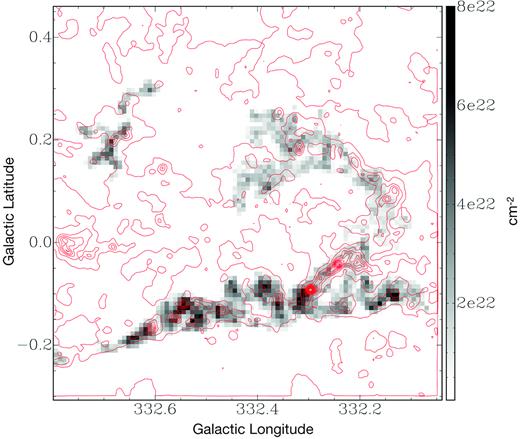
Molecular hydrogen column density from C18O and in red contours N(H2) traced by dust as per Fig. 13.
The emission at 8 μm comes mainly from PAHs (Tielens & Hollenbach 1985) excited by UV radiation from high-mass stars in PDRs. The highest |$8\,\hbox{$\mu $m}$| emission (in Fig. 31) are localized in [SW-R], [SE-R], and [C-R] regions, where the CO spectral lines show the highest emission peaks and the highest velocity dispersion. If the gas in the molecular cloud and the IRDC are part of the same structure, we expect to observe a decreasing gradient in the Tex from [SE-R] to [N-R], similar to that observed from the Southern to Northern cloud (see Table 8).
Taking into account all these factors, we hypothesize that this IRDC arc-like structure, and its extension in the souther ring, is associated with the coldest and densest parts of the cloud, a unique structure along which the star formation activity is at a later stage in the southern ring than the northern ring. Considering [E,SE-R] and [N-R] as the extremities of the IRDC, its length is |${\sim }65\rm \, pc$|.
11 VIRTUAL REALITY AND AUGMENTED REALITY: AN APPLICATION TO RADIO ASTRONOMY
In this section we present a new perspective for looking at astronomical data, developed during the analysis of the G332 molecular ring and applicable to other 3D surveys. The aim is to find a visualization method to better understand the distribution of CO data and to perform an efficient multiwavelength synergy with other surveys. This is not only a data-driven problem but also a data visualization issue, which we tried to solve by experimenting with the use of VR and AR environments and applications.
Currently, the astronomy community is experiencing a growing interest in AR/VR software and hardware to improve data visualization and analysis (Ferrand, English & Irani 2016; Fluke & Barnes 2018). However, most of the software used by astronomers does not offer advanced visualization tools, mainly because it was developed before the current available hardware, but also because its 3D plot capabilities have limited user interaction. On the other hand, the possibility given by VR/AR tools to literally fly through data sets dramatically improves the analysis process. Since our senses evolved in a 3D world, a more intuitive data interpretation is likely to occur in a 3D environment rather than in a 2D representation; this is why immersive techniques have the potential to boost data examination. We made use of VR/AR visualization in our data CO investigation10 to discriminate between emissions related to the main molecular ring structure (as in Section 5.3) and not. Standard 2D datacube plots (as moments maps or PV plots) could lead to data misinterpretations, because of projection effects, while a 3D immersive visualization could help showing data in a greater dimensional space. To solve the above ambiguity, we inspected 12CO, 13CO, and C18O emissions at different thresholds at the same time (2σ, 3σ, 3.5σ, 4σ, and 4.5σ). Such an amount of details is hard to clearly represent on a standard 3D plot, restricting analysis to a limited amount of information.
However, it is important to say that care is needed in PPV 3D datacube inspection since the velocity (or spectral) dimension could lead to misinterpretation in the analysis of the emission morphology (as discussed in Clarke et al. 2018).
A digression on the limits of VR/AR application in astronomy is beyond the purpose of this paper; they were analysed by Vogt & Shingles (2013). Here we note that the continuous increase of computing power, and the consequent increase in smartphone performance, makes it possible to use complex software capable of achieving advanced results without increasing its complexity.
In Appendix A we describe in detail three examples of our VR and AR visualization techniques. All of them are based on the same initial step: convert the fits format into another 3D format, which can be easily read by VR (or AR) frameworks.
12 SUMMARY
We used data from the Mopra Southern Galactic Plane CO Survey of the 12CO, 13CO, and C18O J = 1 → 0 transition lines (Braiding et al. 2018) to perform a morphological and a physical characterization of a GMC (G332 molecular ring) sited in the G332 region of the Galactic plane. The CO emission peaks at VLSR = |$-50\rm \, km\, s^{-1}$|, which is equal to a distance of ∼3.3 kpc from the Sun (assuming correct a near distance solution for KDA) and to a Galactocentric distance of ∼5.5 kpc. The cloud shape is similar to a ring of |${\sim }42\rm \, pc$| in diameter. The total mass of the cloud is estimated in ∼2 × 10⁵ M⊙, assuming [12CO]/[13CO] = 53, [H2]/[12CO] = 1.1 × 10⁴, and uniform Tex = |$30\rm \, K$| for all the subregions of the molecular structure. We found a strong spatial correlation between the C18O and an IRDC structure that was seen as an extinction feature at |$8\,\hbox{$\mu $m}$|.
We derived the Xco variation along the ring for different Tex values, ranging from Xco = 2.1 × 10²⁰ to |$2.3\times 10^{20}\,\mathrm{cm}^{-2}\, \mathrm{K}^{-1}\, \mathrm{km}^{-1}\, \mathrm{s}$|, respectively, for a Tex = |$10\rm \, K$| and for a Tex derived from peak temperature map of 12CO.
We defined an X|$\mathrm{_{CI}^{809}}$| factor, using the [C i] 3P2 → 3P1 transition at 809 GHz and N(H2) traced by 13CO. The derived values are (1.77 ± 0.03) × 1021, (1.83 ± 0.02) × 1021, and |$(1.97\pm 0.02)\times 10^{21}\,\mathrm{cm}^{-2}\, \mathrm{K}^{-1}\, \mathrm{km}^{-1}\, \mathrm{s}$|, respectively, for N(H2) traced by the three assumptions of 12CO, 13CO without adding dark gas, and 13CO adding the dark gas fraction.
The median value of the 12CO/13CO ratio is ∼3.3, with a minimum value close to 1, mostly in the [NW-R], region that we concluded to be the most quiescent part of the cloud. The median [C i]/13CO ratio for the whole cloud is equal to 0.5, ranging in the interval [0.4–1], with the lowest values in [NW-R] and [W-R].
The [C i] emission is lowest in the [NW-R] and [W-R], while the maximum values are found to be in the Southern cloud regions.
The mean dark molecular gas mass fraction of N(H2) not traced by CO results to be equal to |${\sim }16{{\ \rm per\ cent}}$|, in average, considering a Tex = |$20\rm \, K$| for 13CO, and a Tex = |$30\rm \, K$| for [C i].
We compiled a catalogue of clumps decomposing the ring GMC C18O emission and reporting the main physical characteristics derived from CO line, mostly all possess a virial parameter <1.
HiGAL maps were used to derive the dust SED and the N(H2) traced by dust. The derived dust temperature is in the range between 16 and |$27\rm \, K$|. The linear fit between N(H2) traced by dust and the 13CO integrated intensity along all the line of sight gives a coefficient m = |$5.9\times 10^{20}\,\mathrm{cm}^{-2}\, \mathrm{K}^{-1}\, \mathrm{km}^{-1}\, \mathrm{s}$| and b = 9.8 × 1021 cm−2.
We presented a method to disentangle dust emission across the spiral arms from our adopted Galactic model (McClure-Griffiths & Dickey 2007; Vallée 2014), through the use of the 13CO emission along the velocity range |$[-115,-30]\rm \, km\, s^{-1}$| (Table 6).
We found a decreasing gradient in Hi-Gal clumps temperatures and Lbol/Mclump ratio going from [SE-R] towards [N-R], which corresponds to a Tex decrease and to an increase of Xco median value and values dispersion.
The spatial distribution of cold dust and C18O follows an arc-like |$8\,\hbox{$\mu $m}$| extinction feature in northern [SW-R], [W-R], [NW-R], and [E,SE-R]. We found correspondences between the lowest |$8\,\hbox{$\mu $m}$| emission, cold dust, and C18O distribution also in the southern ring. We consider this extinction feature as an IRDC that is inside the molecular ring. Along the IRDC we found that, in general, the peak position of N(H2) traced by C18O present an offset position with respect to N(H2) traced by dust peaks.
We concluded that the observed gas properties are influenced by the stellar formation activity occurring along the identified IRDC, which is an unique structure around which the molecular cloud is wrapped. The path from [E,SE-R] to Southern [N-R] is |${\sim }65\rm \, pc$|. We found evidence of a different star formation activity between the southern and northern ring.
We presented a new visualization approach for the 3D radio astronomy datacubes by using VR and AR environment, based on unity, javascript, and online platforms in combination with non-specifically designed equipment.
ACKNOWLEDGEMENTS
The Mopra radio telescope is part of the Australia Telescope National Facility. Operations support was provided by the University of New South Wales, the University of Adelaide, and Western Sydney University. Many staff of the ATNF have contributed to the success of the remote operations at Mopra. We particularly wish to acknowledge the contributions of Balthasar Indermuehle, David Brodrick, Philip Edwards, Brett Hiscock, and Peter Mirtschin.
Funding for the HEAT telescope is provided by the National Science Foundation under grant number PLR-0944335. PLATO-R was funded by Astronomy Australia Limited, as well as the University of New South Wales, as an initiative of the Australian Government being conducted as part of the Super Science Initiative and financed from the Education Investment Fund. Logistical support for HEAT and PLATO-R is provided by the United States Antarctic Program. We also acknowledge ARC support through Discovery Project DP120101585.
This research made use of astropy, a community-developed core python package for Astronomy (Astropy Collaboration 2013) and the idl astronomy library (Landsman 1995), the simbad data base (Wenger et al. 2000), and aladin sky atlas desktop program (Bonnarel et al. 1999, 2000; Chilingarian & Zolotukhin 2008), maintained by the CDS in Strasbourg, France, and the glue18 (Beaumont, Goodman & Greenfield 2015) visualization package. We thank the anonymous referee for the useful comments that helped us to enrich the work presented in this paper. We would also thank, for the stimulating discussions, Shaila Akhter, Nigel Maxted, Davide Elia, Matthew Freeman, Anant Tanna, and John Lopez.
Footnotes
HEAT is a 62 cm off-axis Gregorian FFTS (Fast Fourier Transform Spectrometer) with heterodyne receivers cooled to |$50\rm \, K$|.
A 2D heat map is a graph in which scatter plot points are encoded in a discrete grid, each cell of the grid has a different colour representing the number of points inside that cell.
https://sketchfab.com/models/57aa5cacc17c4fd2b95516d43669b1f8 shows the 3D model of the 13CO emission represented by two isosurfaces 3D meshes: one at 3.5σ level and one at |$3\rm \, K$|. The mesh grid is 30 arcsec in angular size and |$0.35\rm \, km\, s^{-1}$| in VLSR. In Section 11 we will give a description of how we apply augmented reality to radio data.
We note that 12CO emission in the range |$-44\lt \text{$V_{\mathrm{LSR}}$ }\lt -30\rm \, km\, s^{-1}$|, constrained in the same ring Galactic coordinates, possesses voxels apparently connected to the ring that are not detected by the threshold masks (3σ).
The specific idl command used is smooth.
webvr is an open project to create VR content accessible via the web regardless of the used device; it requires a VR headset, an ios, or android mobile device with accelerometers, and a compatible browser: https://webvr.info/.
https://github.com/borismus/webvr-boilerplate, a framework to develop cross-platform (smartphone with VR headset or desktop VR systems) webvr applications.
At the moment of writing we note that it works on safari and firefox browsers but not on chrome; more informations at https://security.googleblog.com/2017/09/chromes-plan-to-distrust-symantec.html.
REFERENCES
APPENDIX A: HOW TO CREATE VR/AR CONTENT FROM FITS DATACUBES
An example of our VR approach is the 13CO ring emission at 3σ level, presented in a web page we created based on webvr,19 using the webvr boilerplate20 framework. It requires an ios or android device and a VR headset. We will now outline the three steps required to create the VR version of the 13CO ring emission.
![Column densities map for as indicated in the header. With A and B are indicated the column densities derived at a [C i] resolution for an assumed excitation temperature of 30 K. With D and C are indicated the column densities of C18O and 13CO, respectively, computed at the native CO resolution, assuming a Tex derived from the 12CO peak temperature emission.](https://oup.silverchair-cdn.com/oup/backfile/Content_public/Journal/mnras/484/2/10.1093_mnras_sty3510/1/m_sty3510figa1.jpeg?Expires=1749926495&Signature=KzYjJBo4bszaPONcvl8nx~Sr~YnFMJvq5y~p1UWBsQh9eJstiErRdmwBLW2L183L2WcXgMhXJoHpraF7~t0jMeWNgBZzmtoCCDh364U~srZ5imMy7wNHUXjUt85UJQo9JMMlQs651mV4KdIEfZJKIbuN36qguYXwAgS7QaNU5U~-0l~rMpUWkf6WEsNnNtXvO6WYdrCwnJLhncb~4Bcs653z-NGYmdbzLn5r0KklcU8fDbv4luPtvE8ZhQpZ~nUOUlsIFzqGX1UVCk1OFaxsFpAVBE4xQBgfXFPuLCVZ4qK5NB0eYLHwnc~JTaPRK9Ahq7g2Gxp98UR0S9slp0fStg__&Key-Pair-Id=APKAIE5G5CRDK6RD3PGA)
Column densities map for as indicated in the header. With A and B are indicated the column densities derived at a [C i] resolution for an assumed excitation temperature of 30 K. With D and C are indicated the column densities of C18O and 13CO, respectively, computed at the native CO resolution, assuming a Tex derived from the 12CO peak temperature emission.
First step: Convert the fits format to another 3D format. Using a custom python routine based on the mayavi21 package, we extracted a portion of the 13CO 3D fits radio datacube and converted it to wrl22 3D format to make it compatible to other 3D software. A 3D mesh is then created applying a sigma threshold (in this case equal to 3σ) on the extracted datacube section; this mesh is a connected surface (isosurface) that comprises all the voxels whose emission levels are above the threshold. It is important to note that the mesh grid is the same of the starting fits datacube.
Second step: the mesh in wrl format is converted to json 3D format by using the 3D online editor clara.io.23 In this way it becomes readable by the javascript24 library three.js.25 This step is necessary to allow the reading of the 3D model by the webvr boilerplate, which uses three.js library to create VR content.
Third step: web page creation, putting together html and javascript code to configure the webvr environment, linking and setting the 3D json model to three.js javascript library. The final web page is at http://hologhost.altervista.org/VR/index.html. To experience the best view we recommend the use of a pair of VR headset and a smartphone or dedicated VR hardware. We tested it on both ios and android devices.
We verified the coherency between the 3D CO emission distribution, as in the original fits datacube, and the final mesh plotted by three.js in webvr environment. Comparing the mesh grid spacing and the original emission distribution we found no discrepancy between the two representations.
The limit of this method is the impossibility to move inside the VR environment without using a dedicated controller. A solution could be to change the point of view coordinates, but this drastically decreases the interaction rapidity with the model. The advantages are its accessibility and the use of non-proprietary software.
An alternative we explored is based on the sketchfab26 on-line platform,27 which gives the possibility to inspect 3D models both in VR or AR on mobile devices (both ios or android with VR headset) or on desktop PC equipped with VR hardware. This solution is partially free, there is the possibility to choose between a basic or paid accounts, the major difference is on the size limits of the uploaded model. The advantage of this solution is the immediate creation of cross-platform VR and AR environments without any required coding. Here28 there is an AR/VR example of the C18O 3D clumps distribution as reported in Section 9 and in Table A1. The most interesting feature is the AR function accessible via mobile app. In other words it is possible to virtually place the object on a real detected surface and move around it as it is in the real world. Here29 there is a fully navigable 3D representation (VR/AR mode) of the molecular ring 4σ emission coming from all the three CO isotopologues.
Clumps found applying clumpfind to the C18O box smoothed datacube (see Section 5.1 for smooth parameters). In the first column the ID is followed by the flags x, |$v$| indicating that the clump partially extends, respectively, outside the Galactic Longitude interval of the ring or outside the ring velocity range, while or flags means that the clump is outside any of the ring regions (as defined in Fig. 1). The second, third, fourth, and fifth columns are for ℓ b clump centroid coordinates and the angular FWHMs of the corresponding clump ellipsoid, while VLSR is the velocity coordinate and ΔV is its FWHM. Rc is the clump radius, used to derive Mvir under a constant spherical density profile assumption. |$\mathrm{M^{20}_{LTE}}$| is the clump mass computed using the method described in Section 6, for Tex = 20 K and considering C18O emission. αvir is the virial parameter between Mvir and |$\mathrm{M^{20}_{LTE}}$|. |$\mathrm{T^{18}_{AVG}}$|, |$\mathrm{T^{13}_{AVG}}$|, |$\mathrm{T^{AVG}_{12/13}}$| and |$\mathrm{T^{AVG}_{13/18}}$| are, respectively, average Tmb temperatures of the clump in the corresponding line and mean values of the relative lines ratio. |$\mathrm{T^{18}_p}$| is the clump peak brightness temperature in the C18O line emission.
| C18O clumps properties | |||||||||||||||
|---|---|---|---|---|---|---|---|---|---|---|---|---|---|---|---|
| ID | Centroid | Δℓ | Δb | VLSR | ΔV | Rc | Mvir | |$\mathrm{M^{20}_{LTE}}$| | αvir | |$\mathrm{T^{18}_{AVG}}$| | |$\mathrm{T^{13}_{AVG}}$| | |$\mathrm{T^{AVG}_{12/13}}$| | |$\mathrm{T^{AVG}_{13/18}}$| | |$\mathrm{T^{18}_p}$| | |
| ℓ | b | (arcsec) | (arcsec) | |$(\rm \, km\, s^{-1})$| | |$(\rm \, km\, s^{-1})$| | (pc) | (M⊙) | (M⊙) | (K) | (K) | (K) | ||||
| GMCC332.14–0.11x | 332.14° | −0.11° | 325.5 | 132.3 | −52.56 | 2.16 | 3.5 | 3440 | 11 085 | 0.31 | 0.91 | 4.23 | 3.02 | 4.78 | 1.87 |
| GMCC332.19+0.11 | 332.19° | 0.11° | 217.8 | 279.3 | −49.98 | 1.63 | 3.3 | 1824 | 6526 | 0.28 | 0.84 | 4.00 | 2.48 | 4.85 | 1.51 |
| GMCC332.20–0.04 | 332.20° | −0.04° | 272.7 | 269.4 | −48.88 | 1.73 | 2.7 | 2420 | 8474 | 0.29 | 0.79 | 4.24 | 3.02 | 5.41 | 1.29 |
| GMCC332.24–0.13 | 332.24° | −0.13° | 259.8 | 195.6 | −50.72 | 2.05 | 3.2 | 3067 | 9816 | 0.31 | 0.82 | 4.00 | 2.99 | 4.90 | 1.27 |
| GMCC332.28+0.15 | 332.28° | 0.15° | 197.1 | 200.7 | −49.62 | 1.62 | 3.6 | 1652 | 5592 | 0.3 | 0.84 | 3.74 | 1.67 | 4.51 | 1.44 |
| GMCC332.29–0.01|$v$| | 332.29° | −0.01° | 42.3 | 71.7 | −44.83 | 0.63 | 0.9 | 74 | 236 | 0.32 | 0.73 | 2.42 | 2.79 | 3.33 | 0.87 |
| GMCC332.24+0.18 | 332.34° | 0.18° | 168.6 | 210.6 | −49.25 | 1.92 | 2.6 | 2045 | 5000 | 0.41 | 0.89 | 4.27 | 1.86 | 4.86 | 1.47 |
| GMCC332.36+0.20 | 332.36° | 0.20° | 229.8 | 200.7 | −49.25 | 1.91 | 3.9 | 2418 | 5734 | 0.42 | 0.83 | 3.92 | 2.58 | 4.73 | 1.27 |
| GMCC332.37–0.12 | 332.37° | −0.12° | 243.3 | 188.4 | −50.72 | 2.09 | 3.4 | 3159 | 13 253 | 0.24 | 1.03 | 4.59 | 2.78 | 4.54 | 1.98 |
| GMCC332.39–0.09 | 332.39° | −0.09° | 135.6 | 119.4 | −49.62 | 1.37 | 2.3 | 917 | 5504 | 0.17 | 1.20 | 5.06 | 3.39 | 4.29 | 2.53 |
| GMCC332.39+0.11 | 332.39° | 0.11° | 247.5 | 199.5 | −48.14 | 1.39 | 3.4 | 1392 | 7179 | 0.19 | 0.93 | 4.20 | 2.92 | 4.61 | 1.73 |
| GMCC332.39+0.35 | 332.39° | 0.35° | 147.3 | 136.2 | −47.78 | 1.00 | 2.3 | 445 | 1580 | 0.28 | 0.77 | 3.42 | 3.10 | 4.47 | 1.07 |
| GMCC332.42+0.02 | 332.42° | 0.02° | 47.1 | 52.5 | −51.09 | 0.93 | 1.6 | 149 | 380 | 0.39 | 0.80 | 4.42 | 3.51 | 5.58 | 1.11 |
| GMCC332.45–0.10 | 332.45° | −0.10° | 221.4 | 240.6 | −50.35 | 2.50 | 3.6 | 4693 | 9867 | 0.48 | 0.90 | 4.41 | 3.55 | 4.98 | 1.47 |
| GMCC332.50+0.32 | 332.50° | 0.32° | 194.7 | 146.7 | −46.67 | 0.98 | 1.0 | 472 | 2112 | 0.22 | 0.77 | 3.03 | 2.90 | 3.99 | 1.07 |
| GMCC332.55–0.13 | 332.55° | −0.13° | 256.2 | 143.4 | −48.14 | 3.58 | 3.2 | 8571 | 11280 | 0.76 | 1.12 | 5.53 | 3.72 | 5.01 | 2.13 |
| GMCC332.59–0.13 | 332.59° | −0.13° | 186 | 167.4 | −48.88 | 2.92 | 3.0 | 4798 | 4024 | 1.19 | 0.85 | 4.74 | 4.07 | 5.57 | 1.33 |
| GMCC332.62+0.30o | 332.62° | 0.30° | 92.7 | 68.4 | −46.67 | 0.99 | 1.3 | 271 | 1227 | 0.22 | 0.96 | 4.10 | 2.89 | 4.39 | 1.55 |
| GMCC332.65–0.20 | 332.65° | −0.20° | 225.3 | 110.4 | −46.3 | 1.81 | 2.3 | 1599 | 5127 | 0.31 | 1.04 | 4.47 | 2.49 | 4.45 | 2.04 |
| GMCC332.67+0.20o | 332.67° | 0.20° | 64.5 | 35.4 | −47.41 | 0.89 | 0.8 | 138 | 355 | 0.39 | 0.78 | 3.96 | 1.35 | 5.15 | 0.93 |
| GMCC332.70+0.17o | 332.70° | 0.17° | 170.4 | 348.6 | −51.46 | 2.46 | 3.1 | 3981 | 7766 | 0.51 | 0.84 | 2.83 | 2.42 | 3.44 | 1.51 |
| GMCC332.74+0.21|$v$|, o | 332.74° | 0.21° | 132.6 | 88.8 | −44.83 | 1.49 | 3.5 | 755 | 1318 | 0.57 | 0.84 | 3.81 | 2.09 | 4.65 | 1.27 |
| GMCC332.74+0.31o | 332.74° | 0.31° | 93.3 | 91.8 | −45.2 | 0.89 | 1.4 | 237 | 716 | 0.33 | 0.74 | 3.79 | 2.83 | 5.09 | 0.96 |
| GMCC332.79+0.24o | 332.79° | 0.24° | 57.3 | 106.8 | −46.67 | 0.92 | 0.8 | 175 | 383 | 0.46 | 0.77 | 3.85 | 2.50 | 4.97 | 1.09 |
| GMCC332.80–0.23x, |$v$| | 332.80° | −0.23° | 102.9 | 82.2 | −44.46 | 1.40 | 1.4 | 574 | 1058 | 0.54 | 0.98 | 3.71 | 1.47 | 4.04 | 1.84 |
Another approach made use of the unity30 engine to build AR ios applications for both smartphones and tablets. Though giving details on the programming techniques used in this methodology is beyond the purpose of this paper, we report the principal steps through which we created an application usable on mobile devices alone or in combination with a mobile headset system.
The first step is necessarily the conversion of the fits datacube into a readable format for unity. We perform this step using the same custom python routine above mentioned then converting the mesh in obj31 or dae32 3D format. The datacube is thus transformed in a single (or multiple) mesh (depending on how the number of the visualized isosurfaces) ready to be imported in unity. The VR (and AR) capabilities we experimented with made use of the vuforia33 framework, which offers the possibility to create virtual buttons, making possible to build virtual user interfaces through which we interact with the model. The porting on mobile device can be done in unity itself using the vuforia library, depending on the mobile operating system. As expected, we found that the increment in the complexity of the model dramatically slows the visualization experience on mobile devices, even though the meshes corresponding to the 3σ emission of 12CO, 13CO, and C18O, coming from the G332 molecular ring, are easily displayed. Even though we tested this technology on mobile devices, a full immersion visualization experience can be achieved only with dedicated hardware, overcoming the limited computational constraints. On the other hand, the software tools complexity is continuously decreasing, making easier the creation of high-quality full immersion visualization solutions.
