


ABSTRACT
Advances in astronomy are often driven by serendipitous discoveries. As survey astronomy continues to grow, the size and complexity of astronomical data bases will increase, and the ability of astronomers to manually scour data and make such discoveries decreases. In this work, we introduce a machine learning-based method to identify anomalies in large data sets to facilitate such discoveries, and apply this method to long cadence light curves from NASA’s Kepler Mission. Our method clusters data based on density, identifying anomalies as data that lie outside of dense regions. This work serves as a proof-of-concept case study and we test our method on four quarters of the Kepler long cadence light curves. We use Kepler’s most notorious anomaly, Boyajian’s star (KIC 8462852), as a rare ‘ground truth’ for testing outlier identification to verify that objects of genuine scientific interest are included among the identified anomalies. We evaluate the method’s ability to identify known anomalies by identifying unusual behaviour in Boyajian’s star; we report the full list of identified anomalies for these quarters, and present a sample subset of identified outliers that includes unusual phenomena, objects that are rare in the Kepler field, and data artefacts. By identifying <4 per cent of each quarter as outlying data, we demonstrate that this anomaly detection method can create a more targeted approach in searching for rare and novel phenomena.
1 INTRODUCTION
Survey astronomy is producing more data than ever before, both expanding the number of objects observed and the number of observations per object. PanSTARRS, for example, recently delivered to astronomy the first petabyte scale data release (Chambers et al. 2016), Gaia has released data for nearly 2 billion sources (Gaia Collaboration 2016, 2018), and others, like the Transiting Exoplanet Survey Satellite (TESS; Ricker 2014), and the Zwicky Transient Facility (ZTF; Smith et al. 2014), have launched and will release data in short order. The Large Synoptic Survey Telescope (LSST; LSST Science Collaboration 2009) will have first light in the next few years and deliver 10 to 30 terabytes of data per night. These surveys yield unprecedented insights into the universe by observing billions of stars and galaxies through space and time, adding new objects to every category of known phenomena, and creating new categories of previously unknown, unobserved events. Identifying new, anomalous, and outlying observations pose a significant challenge given the scale of data. In this work we present a proof-of-concept for a methodology we’ve developed to address this challenge.
As Douglas Hawkins puts it, ‘An outlier is an observation which deviates so much from the other observations as to arouse suspicions that it was generated by a different mechanism’ (Hawkins 1980). The need for, and by extension the application of, anomaly detection in large-scale astronomy is still relatively new, but anomaly detection is well precedented outside of the astronomical community. Computer scientists have developed techniques to identify abnormalities for a multitude of reasons, including detecting network attacks (Agrawal & Agrawal 2015), fraud (Ahmed, Mahmood & Islam 2016), and malware (Menahem et al. 2009). A survey of different anomaly detection methods is presented by Chandola, Banerjee & Kumar (2009) and initial applications to astronomical survey data have been pursued (for example Wagstaff et al. 2013; Baron & Poznanski 2017). To date, though, discoveries of novel phenomena in astronomy have often been more serendipitous than intentional (see Thompson et al. 2012; Wright et al. 2014; Boyajian et al. 2016). The scale of modern astronomical surveys does not lend itself to discoveries of anomalies by happenstance, rather there must be a concerted effort to mine the data with machine-based methods to have any hope of identifying anomalous, or outlying data.
Broadly speaking, machine learning falls into two categories: supervised and unsupervised learning, which largely relate to the goals of classifying and clustering, respectively (Ivezić et al. 2013). In supervised classification, data are sorted into pre-determined categories that must be taught to the algorithm through well-studied training sets. This method is well suited to quickly identifying objects of known categories with sizable training sets, but is poorly suited to finding rare, novel, or anomalous objects. Finding these sorts of objects after classification generally requires a concerted effort to scour the data. Unsupervised clustering, on the other hand, groups data based on a cluster metric (i.e. proximity or density) in feature space. Unsupervised methods do not require a training set, nor do they require initial categories to create groupings. Likewise, these methods do not carry the implication or requirement of prior knowledge pertaining to any underlying mechanisms driving the measured features. Notably, those mechanisms likely exist (e.g. light curves of Cepheid variables are self-similar because they share an underlying physical cause), and can potentially be discovered as a result of studying clustered data. Anomalies in clustered data are apparent in the form of outlying data, i.e. data that is unclustered.
The strength of unsupervised learning not requiring training data, however, also carries the issue of validation. Particularly in attempting to successfully identify outlying data, there is no simple, universal way to establish a ground truth as anomalies can only be defined in relation to other data. Anomaly detection in astronomy seeks outliers that have the nebulous quality of being scientifically interesting. In this work, we take a look at a single object known to exhibit aberrant behaviour that is of scientific interest: KID 8462852, also known as Boyajian’s star for the first author on its discovery paper. Boyajian’s star was serendipitously discovered to have unusual behaviours by citizen scientists working on Planet Hunters, a Zooniverse project to identify transiting exoplanets in the Kepler data (Boyajian et al. 2016). The discrepant behaviour identified by citizen scientists, asymmetrical dips of varying duration at non-periodic times, can be seen in Quarters 8 and 16 of the Kepler data, shown in the second and fourth panels of Fig. 4. Boyajian’s star also has an observed long-term dimming trend (Montet & Simon 2016; Meng et al. 2017) but is otherwise a typical, main-sequence F3 V star (Teff = 6584 K, log g = 4.124, mass = 1.4 M⊙, radius = 1.699 R⊙). It caught public attention for its odd behaviour, and interest was further fuelled by the potential explanation of this behaviour being due to an alien megastructure (Wright et al. 2014). It has been the subject of intense public and scientific scrutiny, garnering 44 references on ADS between the discovery of its behaviour in 2016 at the time of this writing. As of January 2018, its erratic behaviour has been most consistent with an occulter of ordinary dust (Boyajian et al. 2018).
In this paper, we propose a method for identifying potential outliers in astronomical data bases, and use the behaviour of the well-known, occasionally anomalous source Boyajian’s star as a proof-of-concept by evaluating its identifications in different quarters after applying the methodology described below. In the next section, we discuss the properties of the data we consider: in Section 3 we describe our methods; in Section 4 we present our results on anomaly detection, in which we highlight a small sample of identified outliers including Boyajian’s star; and in Section 5 we discuss future directions and applications of our work.
2 DATA
The data we consider in this study are long-cadence photometric light curves from Quarters 4, 8, 11, and 16 of NASA’s Kepler mission. We utilize Data Release 25 that reprocessed all Q0-Q17 data with the updated data pipeline. We summarize some key features of the Kepler mission and the data we utilize here, but full specifications for Kepler can be found for instrumentation (Van Cleve & Caldwell 2016), data characteristics (Van Cleve et al. 2016), data processing (Jenkins 2017), and the input catalogue (Batalha et al. 2010).1
The Kepler spacecraft was designed to obtain near-continuous photometry for stars in a single, star-rich 105 deg2 field of view (FOV) centred at R.A. = 19h22m40s and Dec = 44°30′00″ from 2009 March to 2013 May. The photometer camera contains 42 CCDs with 2200 × 1024 pixels, where each pixel covers 4 arcsec. However, only pre-selected stars of interest were downloaded (Batalha et al. 2010). The primary goal of the mission was to identify the fraction of terrestrial exoplanets located in the habitable zone of their host star. The Kepler mission took incredibly well-sampled and precise observations, achieving about 30 ppm for solar-type stars (Gilliland et al. 2011, 2015). Stars where an exoplanetary transit signature of around 100 ppm is impossible to detect (i.e. giants, stars fainter than 16th mag, stars in overcrowded fields) were omitted from the target list. Of the roughly half-million targets in the FOV brighter than 16th mag, approximately 30 per cent were targeted. Beyond the primary target list, additional high-priority targets included all known eclipsing binaries in the FOV (>600), all members of open clusters in the FOV, and the nearest main sequence stars. For this work we have utilized the long-cadence observations that are composed of 270, 6.02 s exposures totalling about a half hour per observation and over 4000 observations per epoch. Four times a year, every 3 months, the Kepler spacecraft rolled by 90 deg to re-align its solar panels, and these define epochs known as ‘Quarters’. This will place any given star in one of four different positions on the focal plane depending on season: in this study Quarters 4, 8, and 16 are the same orientation with Quarter 11 in the preceding orientation.
The calibration pipeline for Kepler light curves is optimized towards the goal of identifying exoplanetary transits; light curves for a particular target are not necessarily free from artefacts. The primary means to identify and clean instrumental signatures and systematic errors, the Presearch Data Conditioning pipeline, corrects or removes affected data where possible, but does not perform well for systematics that are non-temporally correlated between targets. Details on the Kepler data processing are available in the Kepler Data Processing Handbook (Jenkins 2017), and known, ongoing phenomena are documented in the Kepler Data Characteristics Handbook (Van Cleve et al. 2016). We do not attempt to remove any remaining artefacts in the Kepler data prior to our analysis, and expect that those artefacts may show up as anomalies (indeed, the identification of artefacts is one of the motivations for this work – in an ongoing survey, such as TESS, the ability to identify artefacts may result in changes to observing that improve mission data quality overall).
We demonstrate our method for this case study on four quarters of data: two that feature Boyajian’s star exhibiting no noteworthy activity or variability (quarters 4 and 11), and two that feature Boyajian’s star exhibiting the unusual behaviour that has attracted the attention and speculation of astronomers world wide (quarters 8 and 16). The data from each quarter is pared down to only the sources that appear in all four quarters to facilitate comparison between quarters.
3 METHODS
In this section, we describe our method for identifying anomalous objects in Kepler data. We begin by processing photometric data into numerical features, detail how we cluster data based on the derived features, and finally discuss how we evaluate outlier identifications.2
We utilize the standard python machine learning package, scikit-learn (Pedregosa et al. 2011), and astropy, a community-developed core Python package for Astronomy (Astropy Collaboration 2013), for the purposes of our analysis. We also make heavy use of scipy packages (Jones et al. 2001) including numpy(Oliphant 2015), matplotlib (Hunter 2007), and pandas (McKinney 2010).
3.1 Feature calculation
The methods here described have been developed for application to the Kepler data, but are applicable to time-series data in general. The data from the Kepler mission are consistently well-sampled and of regular duration; however, astronomical data in general are not. In the interest of eventually applying these methods to sparser data, we treat Kepler data in the same way we would other data. Instead of clustering based on the photometric data itself, we derive a set of 60 numerical features that describe the light curve. These features were created as part of previous data mining work on the Kepler light curves (Walkowicz et al. 2014), several of which are drawn from the features prescribed in Richards et al. (2011) and others developed specifically for Kepler analysis. The features developed and evaluated by Richards et al. (2011) emphasize utility in separating classes of known phenomena and were found to substantially facilitate this. Where features were deemed less important, their inclusion or removal had minimal impact on the results of classification. Initial principle component analyses indicated that more than 40 of the features were required to explain 90 per cent of the variance and we opted to include all features used in the previous Kepler work. The full set of features, and a brief description of each, can be found in Appendix A. Using derived features provides the additional benefit of standardizing clustering compute time after the light curves have been initially processed. Processing a single, long-cadence light curve on a 2.70 GHz Intel Xeon CPU running Linux Ubuntu took 6.7 s on average. Derived features for each object are saved to a pandas data frame by quarter. For clustering, all derived features are scaled to have unit variance and shifted to have a zero mean with scikit-learn’s standardscaler module, but scaled data is not stored.
3.2 Cluster and outlier designation
Cluster input discussed in Section 3.2.
| Variable | Description |
|---|---|
| ε | Radius within which neighbouring points are considered to be associated |
| k | Minimum number of neighbours within ε to qualify a point as part of a cluster |
| i | Index of a point in the data |
| j | Place-holding integer |
| n | Size of range to consider when determining location of elbow |
| di, j | Distance to the jth nearest neighbour of the ith point |
| Ntotal | Size of the entire data set |
| Nsample | Size of the data set sampled for ε determination |
| S | The set of all potential elbow points, defined in equation (2) |
A point may be a core cluster member if it has the minimum number of neighbours within the radius ε, an edge cluster member if it contains fewer than k neighbours but has at least one neighbour within ε that is a core cluster member, or an outlier if it does not contain enough neighbours within the cutoff and no neighbours within ε are themselves core cluster members. As density is defined as the number of samples within a given volume, small changes in the ε can produce significantly different clustering results.
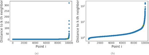
A sample of data from Quarter 4. A clear elbow can be seen in the plots illustrating the distance to the kth neighbour. The point in green represents the elbow found by the method described in Section 3.1. The points in orange are the points before and after the elbow. (a) shows the entire sample, (b) the elbow in log-scale.
In the data we have considered, which is scaled to unit variance on each feature, distance to the fourth neighbour is consistently flat until the elbow. In the case of the sampled 104 points, we look at 0.2 per cent of values on either side of each point (20 points). The elbow is determined to be the first point where the average of the following values is at least 5 per cent greater than the preceding average. This definition is less sensitive to point-to-point variation and is prone to catch the early edge of the elbow as in Fig. 1(a). By pre-empting the elbow a bit and finding lower value of epsilon, cluster membership is more exclusive ensuring data after the true elbow is outliers and more objects on the edge are identified as edge cluster members. We find this preferable to a larger epsilon which would lead to increased core cluster membership and fewer outliers.
3.3 Dimensionality reduction and outlier evaluation
The focus of this initial work is to produce an initial list of outliers and evaluate how this method performs using Boyajian’s star as an example. Beyond this, we examine and present a small sample of outlying objects from the full list of outliers produced. We have developed a user interface for visualization and data exploration in python 2.7. Data exploration relies on a reduction of the data to a 2D representation that maintains clustering relationships. In the GUI, we tie the reduced data to the original light curves to explore different clusterings and outliers; selecting a point in the reduction displays that point’s associated light curve and it’s Kepler ID. An example showing Boyajian’s star selected in Quarter 16 can be seen in Fig. 2.
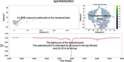
This GUI facilitates exploration of the data. A user can click on any outlying point in the t-SNE reduced plot and the light curve for that object will be displayed in the bottom. Outliers are scattered points in red and clustered data have been log-scale hex-binned into a 35x35 grid to illustrate cluster density. Over 96 per cent of objects are concentrated in the core cluster.
The clustering method we’ve used, detailed in Section 3.2, determines clusters based on density by considering nearest neighbours. In visually representing the high dimensional feature space of the data, we have found the most illustrative reductions focus on maintaining nearest neighbour relationships. One of the best methods for this particular need is t-SNE (t-distributed Stochastic Neighbourhood Embedding; Van Der Maaten & Hinton 2008). As well as it can, t-SNE preserves the relative proximity of nearest neighbours (via a similarity score) with the consequence of exaggerating the distance of other data points. This is accomplished by calculating similarity scores between points of the full-dimensional set and generating a uniform random distribution in the desired dimensionality assigning each random point to a corresponding data point. The algorithm then calculates the similarity scores for the low dimensional distribution and the differences between the scores for each point, and uses that difference to move each point towards, or away from each other point in the low dimensional space, and this is repeated until the Kullback–Leibler divergence is minimized. As t-SNE is computationally expensive, it was necessary to break the larger data set, on the scale of 105, into smaller, 104 scale chunks. Unfortunately, the reduction of a sample cannot be simply generalized to a larger population. Since t-SNE fundamentally relies on an n-body simulation, inclusion of additional data would affect the resulting positions of all points. With that limitation noted, only clustered data has been omitted and subsets of data have proven effective in illustrating clusters and outlier relationships. In following plots, a common sample is used between all four quarters with clustering done on the full quarters. This sample was chosen with two primary considerations: every object identified as an outlier in any quarter are included, plus 104 points are randomly sampled from the remaining objects that were consistently clustered. In each of the full quarters, around 95 per cent of the objects are clustered, while clustered objects constitute only around two-thirds of each quarter’s sample.
We visually inspect the t-SNE reduced data and cluster determinations. We display their light curves to determine if outlier classifications are justified using a GUI developed for exploration as shown in Fig. 2. We assess the ‘movement’ of individual points in the feature space from quarter to quarter to better understand what type of an outlier each point is as it appears that smaller movements correspond to noise and measurement errors, and larger movements to more drastic feature differences.
4 RESULTS AND DISCUSSION
We discuss the results of our outlier identification method first as a whole, then by quarter. We evaluate how this performed for our proof-of-concept case, Boyajian’s star, and finally we discuss a sample of objects from the outliers including some of the most noticeable outliers from the reduction.
Across all quarters we considered 149 789 objects, of which 8507 unique objects were identified as outliers representing 5.68 per cent of all objects considered. A total of 141 282 objects, 94.32 per cent of all objects, were identified only as part of a cluster, either as core cluster members or edge cluster members. Objects that were identified as outliers in every quarter constituted 3584 of the outliers (2.39 per cent of all objects and 42 per cent of all outliers), and the remaining 4923 objects were found to be transient outliers, identified as an outlier and as a cluster member at least once each in different quarters. We summarize the designations made overall in Table 2 and by quarter in Table 3.
Outlier summary.
| Description | Count | Percent of total objects (per cent) | Percent of outliers (per cent) |
|---|---|---|---|
| Total outliers | 8507 | 5.68 | – |
| Outliers in every quarter | 3584 | 2.39 | 42.13 |
| Transient outliers | 4923 | 3.29 | 57.87 |
| Description | Count | Percent of total objects (per cent) | Percent of outliers (per cent) |
|---|---|---|---|
| Total outliers | 8507 | 5.68 | – |
| Outliers in every quarter | 3584 | 2.39 | 42.13 |
| Transient outliers | 4923 | 3.29 | 57.87 |
Designations by quarter.
| Quarter | Core cluster members | Edge cluster members | Outliers |
|---|---|---|---|
| (per cent of total population) | (per cent of total population) | (per cent of total population) | |
| Q4 | 142 534 | 2389 | 4866 |
| (95.16 per cent) | (1.59 per cent) | (3.25 per cent) | |
| Q8 | 142 235 | 2510 | 5044 |
| (94.96 per cent) | (1.68 per cent) | (3.37 per cent) | |
| Q11 | 140 933 | 2977 | 5879 |
| (94.09 per cent) | (1.99 per cent) | (3.92 per cent) | |
| Q16 | 141 129 | 2910 | 5750 |
| (94.22 per cent) | (1.94 per cent) | (3.84 per cent) |
List of outliers.
| KID | RA | Dec | Teff | Teff err | Teff err | log g | log g err | log g err | Kepmag | Q4 | Q8 | Q11 | Q16 |
|---|---|---|---|---|---|---|---|---|---|---|---|---|---|
| (K) | (K) | (K) | |||||||||||
| 757099 | 19 24 10.334 | + 36 35 37.72 | 5519 | 182 | −149 | 3.82 | 0.64 | −0.21 | 13.15 | −1 | −1 | −1 | −1 |
| 757450 | 19 24 33.024 | + 36 34 38.57 | 5332 | 106 | −96 | 4.50 | 0.05 | −0.04 | 15.26 | 0 | 1 | −1 | 0 |
| 892376 | 19 24 15.329 | + 36 38 08.92 | 3973 | 124 | −152 | 4.66 | 0.06 | −0.02 | 13.96 | −1 | −1 | −1 | −1 |
| 893507 | 19 25 15.007 | + 36 37 59.62 | 5382 | 177 | −144 | 3.92 | 0.67 | −0.29 | 12.52 | −1 | 1 | −1 | −1 |
| 893647 | 19 25 21.108 | + 36 41 24.86 | 4856 | 146 | −131 | 4.58 | 0.06 | −0.04 | 15.28 | −1 | 1 | −1 | −1 |
| 1025986 | 19 24 08.086 | + 36 46 15.75 | 5604 | 84 | −67 | 4.23 | 0.21 | −0.11 | 10.15 | −1 | 1 | 1 | −1 |
| 1026032 | 19 24 10.577 | + 36 43 45.38 | 5951 | 160 | −178 | 4.64 | 0.03 | −0.13 | 14.81 | −1 | −1 | −1 | −1 |
| 1026474 | 19 24 35.786 | + 36 43 25.75 | 4276 | 150 | −165 | 4.60 | 0.05 | −0.02 | 15.28 | 1 | −1 | −1 | −1 |
| 1026861 | 19 24 56.220 | + 36 43 44.62 | 7063 | 74 | −95 | 4.04 | 0.14 | −0.11 | 11.00 | 0 | −1 | −1 | −1 |
| 1026957 | 19 25 01.078 | + 36 44 37.00 | 4859 | 97 | −97 | 4.61 | 0.02 | −0.05 | 12.56 | 0 | 0 | 0 | −1 |
Note: For Q4, Q8, Q11, and Q16: −1 indicates that an object is outlying in that quarter, 0 core cluster membership, and 1 that an object is an edge cluster member. Full, machine readable table available at https://github.com/d-giles/KeplerML/blob/paperwork/KIC_Outlier_Properties.csv.
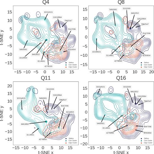
We examine the relationships between clustered, edge of cluster, and outlier data in Fig. 3. We separate each quarter into the different designations, representing each group with a different Kernel Density Estimate (KDE) plot. While these reductions are limited to a sample only and do not contain the entirety of the data, they are still a helpful visual guide to the data relationships. The general shapes of each KDE plot for each of the designations seem to be fairly consistent, even in Quarter 11 that has the same general form but is lopsided.
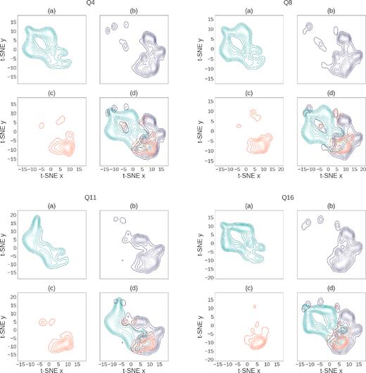
Above, we visualize each quarter with a common sample to illustrate how clustered data and the outlying data relates to each other within each quarter. We have chosen the sample such that all objects that are identified as outliers in at least one quarter have been included (8507 objects), alongside 10k additional objects randomly sampled from the remaining data. Outliers constitute up to a third of the data in each quarter’s sample; however, in the full Quarter about 96 per cent of light curves are clustered and only only up to 4 per cent are identified as outliers. We cluster the full data in 60-D feature space, use t-SNE to represent the sample in 2D, and show the density of data using three Gaussian Kernel Density Estimates for each quarter. In each subplot (a) shows the KDE for the clustered data of that quarter in blue, (b) shows the KDE for outlying data in purple, (c) shows the KDE for edge-of-cluster data in orange, and (d) shows all three KDEs overplotted. Lighter coloured lines indicate higher density regions.
4.1 Results for Boyajian’s star
As mentioned in Section 1, we considered Boyajian’s star as a proof-of-concept case to evaluate whether or not our method would be able to recreate the serendipitous discovery of anomalous behaviour made by human evaluation. As can be seen in Fig. 4, our method was able to identify Boyajian’s star as an outlier only where odd behaviour existed, proving consistent with previous human evaluation. Finding genuine outliers and anomalies of potential interest in hundreds of thousands of sources by circumstance is not trivial, but neither is it impossible (as evidenced by the discovery of Boyajian’s star). As we move to millions and billions of sources per survey, however, it becomes much less likely that scientists, or even crowd-sourced searches, will turn up serendipitous discoveries. The method we have developed has identified less than 4 per cent of the objects as outlying in any given quarter, significantly more manageable than the whole data set. Coupled with the inclusion of genuine anomalous data like Boyajian’s star, this indicates that our methodology can significantly facilitate these discoveries.
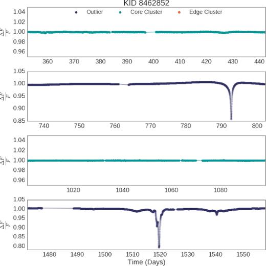
Here we can see that our method has successfully identified the behaviour of Boyajian’s star in each quarter. It has only been identified as an outlier in the quarters also noted by scientists and citizen scientists as anomalous (Boyajian et al. 2016).
In Fig. 5 we look at Boyajian star’s position relative to other data in each quarter. In Quarters 4 and 11 where Boyajian’s star exhibits no aberrant behaviour, it falls neatly into the core clustered data. In Quarters 8 and 16, Boyajian’s star can be found outside the core cluster, illustrating its identification as an outlier.
Here we highlight 10 objects that have been identified as an outlier in at least one quarter. Three of these objects are outliers in all quarters and the remaining objects are transient outliers that are identified in one or more quarters as an outlier, but not in all quarters. Boyajian’s star, KID 8462852, itself is a transient outlier in Quarters 8 and 16 but as a core cluster member in Quarters 4 and 11, its light curves can be found in Fig. 4.
4.2 Example outlier objects
Here we show a few example objects semirandomly selected from the larger sample of outliers. These examples have been selected to include objects that were identified as outliers in all quarters, some that were identified as an outlier in only one quarter, and others with multiple outlier identifications. Notably, they were not individually selected as specific types of outliers and are presented largely without thorough investigation into the origin of their anomalous behaviour. They are provided purely to illustrate a small sample of the outlying data. In Fig. 5 we highlight the example outlier object excepting the most outlying objects discussed in Section 4.2.1 as their positions in the reduction are significantly removed from the rest of the data.
4.2.1 Anomalous phenomena
When we examine the t-SNE reduced data, there are three objects that stand out more than any others: KIC 7679979, KIC 7446357, and KIC 7659570 (Fig. 6). KIC 7679979 exhibits extreme behaviour in only Quarter 4. On inspection of its light curve, this does not seem to be due to astrophysical mechanisms, rather it seems more likely to be an artefact and is discussed further in Section 4.2.4.
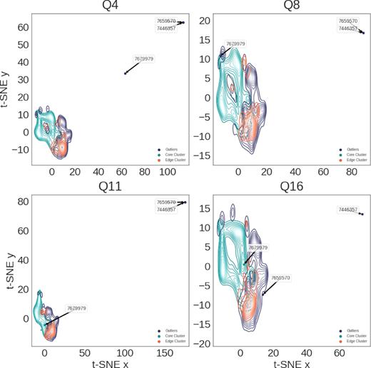
Three objects in this sample extend well beyond all other data in the t-SNE reduction. Two of these, KID 7446357 and KID 7659570, are extreme outliers in all quarters and their light curves are shown in Figs 7(a) and 8(b), respectively. These two objects are SU-Uma cataclysmic variables. KID 7679979 is an extreme outlier only in quarter 4, its light curves are shown in Fig. 10(c) and is included in the discussion of artefacts in Section 4.2.4.
KICs 7446357 and 7659570 are V1504 Cyg and V344 Lyr, respectively. Light curves for these objects are shown in Fig. 7. These stars have been identified as VW Hydri, a subclass of SU-UMa Cataclysmic Variables, itself a subclass of dwarf novae distinguished by superhumps (Kato et al. 2004; Cannizzo et al. 2012). These stars, and the dwarf nova class of stars in general, have been the subject of extensive study for the past century as these semidetached binary systems present unique, periodic outburst behaviours. The first reference to V1504 Cyg comes from Kukarkin et al. (1977) and discovery of V344 Lyr from Hoffmeister (1966). Both appear in the original A catalog and Atlas of Cataclysmic Variables by Downes & Shara (1993). Cannizzo et al. (2012) present a study of the outburst properties of these two CVs contained in the Kepler field.
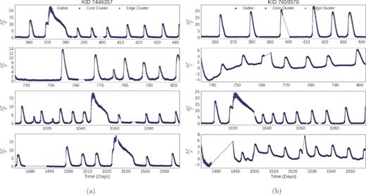
SU-Uma cataclysmic variables have extreme features, are very rare in the Kepler data set, and are identified as outliers by our method. (a) KIC 7446357 has been identified as an SU Uma cataclysmic variable and as an outlier in each quarter. (b) KIC 7446357 has been identified as an SU Uma cataclysmic variable and as an outlier in each quarter. In Quarters 8 and 16, the normalized flux of KIC 7659570 is negative in the first 20 d. These negative fluxes appear to coincide with an outburst at the start of those observation cycles.
4.2.2 Rare objects
As we search for anomalies, we are, by definition, searching for rare objects. Rarity is determined by the data each object is compared to. When looking at a subset of data, the rarity of different objects may differ from their rarity in the full set. Three of the outliers from our example objects have been identified as eclipsing binary stars, KID 3102000, KID 7960547, and KID 11619964. Notably, none of these three objects were found to be core cluster members in any quarter. This would suggest that binary stars are relatively rare in the Kepler data set. The Kepler Eclipsing Binary Catalogue contains 2878 entries at the time of this writing, accounting for only 1.3 per cent of Kepler objects (Kirk et al. 2016). KIC 3102000 is a highly eccentric, long period, detached eclipsing binary system of spectral type G1V (Teff = 5933 K), with a period of 57.06 d. It was identified as a Kepler Object of Interest (KOI) with clear transit activity by Tenenbaum et al. (2012), but Dong, Katz & Socrates (2013) later recognized that it was, in fact, an eclipsing binary with a highly eccentric (emin = 0.73) period. The light curve for KIC 3102000 is shown in Fig. 8(a).
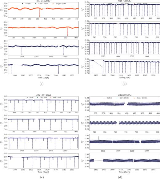
Objects that are relatively rare within the Kepler data set, like eclipsing binaries in (a), (b), and (c) and the B-type star in (d), are determined to by outliers by our method. (a) KIC 3102000 is identified as a long-term eclipsing binary and as an outlier in Quarters 11 and 16. (b) KIC 7960547 shows standard behaviour for an eclipsing binary. (c) KIC 11619964 exhibits standard behaviour for an eclipsing binary with regular transits of two unique depths. (d) KIC 8233804 B type star. Its variability is likely due to rotation or binarity (McNamara, Jackiewicz & McKeever 2012).
KIC 7960547 was identified as a detached eclipsing binary with a transit period of 6.767 d by Prsa et al. (2011) in the first comprehensive catalogue of eclipsing binaries for the Kepler field and as a KOI based on transit activity (Teff = 5669 K, T1/T2 = 0.94428, R1 + R2 = 0.07233R⊙, and sin i = 1.00059; Fig. 8b).
KIC 11619964 was identified as a detached eclipsing binary with a transit period of 10.368 d by Prsa et al. (2011) in the first comprehensive catalogue of eclipsing binaries for the Kepler field and had properties refined by Slawson et al. (2011) (Teff = 5582 K, log g = 4.42, T1/T2 = 0.87462, R1 + R2 = 0.09842⊙, and sin i = 0.99486; Fig. 8c).
KIC 8233804 is a main sequence B9V star(Teff = 11068 K, log g = 4.377, mass = 2.102 M⊙, and radius = 1.555R⊙). As discussed in Section 2, the Kepler Input Catalogue is curated to find exoplanets and there are very few B-type stars. McNamara et al. (2012) studied 252 B-star candidates and classified this object’s variability due to rotation or binarity rather than pulsations given its relative smoothness. The light curve for KIC 8233809 is shown in Fig. 8(d).
4.2.3 Edge of cluster outliers
There is a particular challenge in clustering associated with sparsity at cluster edges that makes the distinction between clustered data and unclustered data nebulous. In Gaussian distributions, a majority of data lies near the mean with sparser data in the tails. Any cluster with one or more Gaussian distributed features will inevitably have an uneven density with sparser data at the edges. Two objects, KID 3547996 (Fig. 9a) and KID 4276000 (Fig. 9b), are sometimes identified as outliers, and as edge cluster members at other times. These two objects exist on the edge of the clustered data, oscillating from quarter to quarter in relation to other data. Rather than being truly anomalous, these would appear to vary in designation due to the relative sparsity at the edge of the cluster.
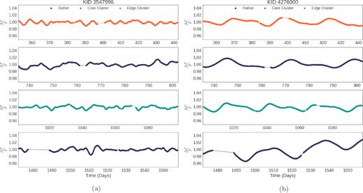
Some objects are identified as outliers, core cluster members, and edge cluster members. An examination of the reductions in 5 show that these objects maintain similar relationships relative to the rest of the population in each quarter, consistently on the edge, fluctuating between outlier and cluster members. (a) KIC 3547996 is identified as an outlier in Quarters 8 and 16. This object has been identified as a star by the GAIA (Gaia Collaboration 2016). (b) KIC 4276000 moves between all identifications and appears as an outlier twice in Quarters 8 and 16. It has been identified as a rotationally variable star by Debosscher et al. (2011).
KIC 3547996 is contained in the Simbad data base as TYC 3134-24-1 from the Tycho-2 Catalogue of the brightest 2.5 million stars and as 2MASS J19291519 + 3841290. This star appears to be a K7 III giant (Teff = 4023 K, log g = 1.091, mass = 1.63M⊙, and radius 60.23R⊙). The light curve for KIC 3547996 is shown in Fig. 9(a).
KIC 4276000 appears to be a G6 IV subgiant (Teff = 5510 K, log g = 3.508, mass = 1.79M⊙, and radius = 3.901R⊙). This object was classified by Debosscher et al. (2011) as a rotationally variable star following the Q0 and Q1 data release via an automated method, a new classification made by this paper unique from other sources of stellar variability. The light curve for KIC 4276000 is shown in Fig. 9(b).
4.2.4 Data Artefacts
In addition to finding novel or rare phenomena, anomaly detection can be useful in finding aberrant data caused by processing. This can help refine data processing techniques, clean data bases of corrupt data, and reveal unaccounted for systematics. Several of the identified outliers, KID 3114661 (Fig. 10a), KID 5460981 (Fig. 10b), KID 7679979 (Fig. 10c), and KID 10334631 (Fig. 10d), are core cluster members except for quarters where features would appear to be related to data artefacts rather than the behaviour of the objects themselves.
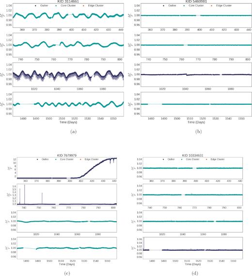
Many of the outliers our method identified exhibit features that appear to be artefacts from data processing or collection, rather than behaviours of the objects themselves. In either case, our method is able to identify objects with anomalous behaviour. (a) KIC 3114661 shows exaggerated features in Quarter 11, apparently related to the quarterly roll that Kepler performed. (b) KIC 5460981 is identified as an outlier only in Quarter 11 where there is odd jump around day 1040. (c) KIC 7679979 exhibits odd behaviours in Quarters 4 and 8 that are not present in any other quarter. (d) KIC10334631 has an odd jump at the beginning of Quarter 16, where it is identified as an outlier.
KIC 3114661 appears to be a G7 VI subdwarf (Teff = 5243 K, log g = 4.674, mass = 0.69M⊙, and radius = 0.635R⊙). It was identified in a study by Walkowicz & Basri (2013) as a rotationally variable star and as a potential planet candidate. This was identified later by Coughlin et al. (2014) to be a false-positive via ephemeris through direct pixel response function and by Morton et al. (2016) by calculation of the False Positive Probability. KID 3114661 exhibits a persistent and periodic variance that is exaggerated in Quarter 11. Examining other quarters of this objects data reveals that this behaviour coincides neatly with the quarterly roll that Kepler performed. The light curve for KIC 3114661 is shown in Fig. 10(a).
KIC 5460981 is a main sequence F5 V star (Teff = 6692 K, log g = 4.275, mass = 1.26M⊙, and radius = 1.351R⊙). McQuillan, Mazeh & Aigrain (2014) determined this object to have no significant period detection or transit features. The light curve of KID 5460981 shows an odd jump around day 1040. The light curve for KIC 5460981 is shown in Fig. 10(b).
KIC 7679979 appears to be a main sequence G3VI subdwarf (Teff = 5693 K, log g = 4.551, mass = 0.95M⊙, and radius 0.856R⊙) with no previously documented variability or properties of note. The light curve of KID7679979 exhibits abnormal brightening at the end of Quarter 4 and shows some odd spikes in Quarter 11 around days 740 and 750, as can be seen in Fig. 10(c). This object is identified only as a star by McQuillan et al. (2014). This does not appear to coincide with any known phenomena nor do either of these behaviours present themselves in other quarters.
KIC 10334631 appears to be a K1VI subdwarf (Teff = 4991 K, log g = 4.631, mass = 0.852M⊙, and radius = 0.944R⊙). KID10334631 exhibits an individual, bright observation exceeding a 6 per cent increase around day 1470. The light curve for KIC 10334631 is shown in Fig. 10(d).
4.3 Discussion
These example outliers show that our method is adept at identifying anomalous behaviour where it occurs including rare objects within a data set and data potentially corrupted. Notably, however, not every outlier identified exhibited behaviour we might recognize as anomalous. Objects on the edge of clusters that do not exhibit particularly interesting behaviour, are identified as outlying due to the non-uniform density of data given the features we consider. This poses a problem for our method, as we define a cluster based on its density. However, the consistency of relative position from quarter to quarter for such objects may present an opportunity to utilize intraquarter movement to further characterize an object’s outlying nature. This method effectively pares data sets down to the most promising potential objects containing anomalous behaviour. It does not, however, have the ability to identify the cause of this behaviour or the ability to predict what objects might be of interest. The use of this method is to supplement surveys by focusing the search for novel phenomena and data anomalies to a manageable size, so that as data is made available, additional observation may be focused more effectively.
5 CONCLUSIONS AND FUTURE WORK
We have demonstrated the effectiveness of our method on Kepler data by successfully identifying anomalous behaviour of Boyajian’s star in addition to showing how this method can quickly identify interesting subsamples (like eclipsing binaries), truly unique, or rare objects (cataclysmic variables, Boyajian’s star, or data artefacts). We have also seen that in an individual quarter, the list of outliers will contain objects that consistently reside on or near the edge of clustered data, but which do not present anomalous behaviour. This demonstrates a limitation of the methodology, clusters are defined to have constant density, but evidently do not. Gaussian distributions within clustered data lead to sparser regions at the edges of clusters. Problematically, this also appears to be where some of the genuinely anomalous data resides. We see, though, that a potential solution presents itself if we examine intraquarter movement.
Following this work, we will examine outlier distributions in more depth with particular attention paid to formalize outlier scoring. Having established the utility of this method using a feature set curated for classification and datamining, we will evaluate the utility of features in the interest of maximizing impact while reducing computational cost. We will examine the utility of other outlier identification methods as well, and apply these methods to the full Kepler data set of long cadence light curves. We also intend to apply our method to other time-series data as they become available, including the TESS, and eventually LSST. As larger scale surveys release data, computational methods will be relied upon to identify novel sources. Wagstaff et al. (2013) identify the need to not only develop methods of outlier identification and rank, but further to develop a diversity of methods to highlight outliers of different types and of different origins as we seek to enable scientific discovery through data prioritization.
SUPPORTING INFORMATION
Table 4. List of Outliers.
Please note: Oxford University Press is not responsible for the content or functionality of any supporting materials supplied by the authors. Any queries (other than missing material) should be directed to the corresponding author for the article.
ACKNOWLEDGEMENTS
DG acknowledges the support of the Illinois Space Grant Consortium Graduate Fellowship and thanks the LSSTC Data Science Fellowship Program, his time as a Fellow has benefitted this work. LW thanks the New Frontiers in Astronomy and Cosmology grant, administered by Don York of the University of Chicago and funded by the John Templeton Foundation, for support of initial development of the methods used herein, and collaborators Revant Nayar, Ed Turner, Jeff Scargle, Vikki Meadows, and Tony Zee for their contributions to this project’s inception. All of the data presented in this paper includes data collected by the Kepler mission and were obtained from the Mikulski Archive for Space Telescopes (MAST). STScI is operated by the Association of Universities for Research in Astronomy, Inc., under NASA contract NAS5-26555. Funding for the Kepler mission is provided by the NASA Science Mission directorate. Stellar properties reported are the revised stellar properties of Kepler targets reported by Huber et al. (2014) except where otherwise noted, accessed through the NASA Exoplanet Archive, operated by the California Institute of Technology under contract with the National Aeronautics and Space Administration under the Exoplanet Exploration Program. This research has made use of the SIMBAD data base, operated at CDS, Strasbourg, France (Wenger et al. 2000).
Software: scikit-learn (Pedregosa et al. 2011), astropy (Astropy Collaboration 2013), scipy(Jones et al. 2001), numpy (Oliphant 2015), matplotlib (Hunter 2007), and pandas (McKinney 2010).
Footnotes
These resources are available via the Mikulski Archive for Space Telescopes at http://archive.stsci.edu/kepler/.
Our code is made publicly available at https://github.com/d-giles/KeplerML.
REFERENCES
APPENDIX A: FEATURES
Features.
| Feature | Code reference | Description |
|---|---|---|
| Long-term trend | longtermtrend | Linear trend of fluxes over whole series |
| Mean to median ratio | meanmedrat | Ratio between the mean and the median |
| Skewness of fluxes | skews | Skewness of the fluxes |
| Variance | varss | Variance of the fluxes |
| Coefficient of variability | coeffvar | Ratio of the standard deviation to the mean of the fluxes |
| Standard deviation | stds | Standard deviation of the fluxes |
| Number of outliers beyond 1σ | numout1s | Count of flux values beyond 1σ deviation from the mean |
| Number of negative outliers | numnegoutliers | Count of flux values beyond 4σ deviation from the mean, less than the mean |
| Number of positive outliers | numposoutliers | Count of flux values beyond 4σ deviation from the mean, greater than the mean |
| Number of outliers | numoutliers | Count of total flux values beyond 4σ deviation from the mean |
| Kurtosis | kurt | Kurtosis of the fluxes |
| Median absolute difference | mad | Median absolute difference from the median flux |
| Maximum slopes | maxslope | Value defining the 99th percentile of slopes between 2 sequential fluxes |
| Minimum slopes | minslope | Value defining the 1st percentile of slopes between 2 sequential fluxes |
| Mean of postive slopes | meanpslope | Mean of positive slopes between 2 sequential fluxes |
| Mean of negative slopes | meannslope | Mean of negative slopes between 2 sequential fluxes |
| G asymmetry | g_asymm | Ratio of mean positive slopes to negative slopes (large dummy value of 10 given if no negative slopes) |
| Rough g asymmetry | rough_g_asymm | Ratio of number of positive slopes to negative slopes (large dummy value of 10 given if no negative slopes) |
| Diffence asymmetry | diff_asymm | Difference between the mean of the positive slopes and the absolute mean of the negative slopes |
| Skewness of slopes | skewslope | Skewness of slopes |
| Slopes mean value | meanabsslope | Mean of the absolute value slopes |
| Variance of absolute slopes | varabsslope | Variance of the absolute value slopes |
| Variance of the slopes | varslope | Variance of the slopes |
| Absolute mean of the second derivative | absmeansecder | Mean of the absolute second derivative of the fluxes |
| Number of positive spikes | num_pspikes | Count of positive spikes as defined by a positive slope 3σ or greater than the mean positive slope |
| Number of negative spikes | num_nspikes | Count of negative spikes as defined by a negative slope 3σ or smaller than the mean negative slope |
| Number of positive second derivative spikes | num_psdspikes | Count of second derivative values beyond 4σ deviation from the mean of second derivative values, greater than the mean |
| Number of negative second derivative spikes | num_nsdspikes | Count of second derivative values beyond 4σ deviation from the mean of second derivative values, less than the mean |
| Standard deviation ratio | stdratio | Ratio of the standard deviation of the positive slopes to the standard deviation of the negative slopes (large dummy value of 10 given if negative standard deviation is zero) |
| Pair slope trend | pstrend | Ratio of positive slopes with a subsequent positive slope to the total number of slopes |
| Number of ‘zero’ crossings | num_zcross | Count of occurences where sequential observations cross the longterm trendline |
| Number of ‘plus-minus’ slope switches | num_pm | Count of slope transitions from positive to negative |
| Length of naive maxima | len_nmax | Count of naive maxima where a maxima is the largest flux value within 10 points on either side |
| Length of naive minima | len_nmin | Count of naive minima where a minima is the smallest flux value within 10 points on either side |
| Maxima autocorrelation coefficient | mautocorrcoef | Autocorrelation coefficient of one maxima to the next |
| Peak-to-peak slopes | ptpslopes | Mean of the slopes from naive peak-to-peak |
| Periodicity | periodicity | Coefficient of variability for time-differences, ratio of the standard deviation to the mean of time-difference between maxima |
| Periodicity residual | periodicityr | Coefficient of variability for time-differences of maxima using residuals |
| Naive periodicity | naiveperiod | Mean of the time-differences between naive maxima |
| Maxima variation | maxvars | Coefficient of variation of the maxima, ratio of the standard deviation to the mean of the naive maxima flux values |
| Maxima variation residuals | maxvarsr | Coefficient of variation of maxima flux values using residuals instead of standard deviation |
| Odd to even ratio | oeratio | Ratio of odd indice minima flux values to even indice means flux values |
| Amplitude analogue | amp_2 | Peak-to-peak based on 1st and 99th percentile |
| Normalized amplitude analogue | normamp | amp_2 divided by the mean flux value |
| Median buffer percentile | mbp | Fraction of the number of points within 10% of the amplitude to the median |
| Ratio of flux percentiles (60th to 40th) | mid20 | Ratio of flux percentiles (60th to 40th) over (95th to 5th) |
| Ratio of flux percentiles (67th to 32nd) | mid35 | Ratio of flux percentiles (67th to 32nd) over (95th to 5th) |
| Ratio of flux percentiles (75th to 25th) | mid50 | Ratio of flux percentiles (75th to 25th) over (95th to 5th) |
| Ratio of flux percentiles (82nd to 17th) | mid65 | Ratio of flux percentiles (82nd to 17th) over (95th to 5th) |
| Ratio of flux percentiles (90th to 10th) | mid80 | Ratio of flux percentiles (90th to 10th) over (95th to 5th) |
| Percent amplitude | per centamp | Largest absolute difference between the max or min flux and the median (as apercentage of the median) |
| Maximum ratio | magratio | Ratio of the maximum flux value to amp_2 |
| Auto-correletion coefficient | autocorrcoef | Auto-correlation coefficient of the fluxes |
| Slopes autocorrelation coefficient | sautocorrcoef | Auto-correlation coefficient of the slopes |
| Flatness mean around naive maxima | flatmean | Mean average of flatness values around maxima, where flatness is the mean of the absolute value of 6 slopes on either side of each maxima |
| Flatness mean around naive minima | tflatmean | Mean average of flatness values around minima, where flatness is the mean of the absolute value of 6 slopes on either side of each minima |
| Roundness mean around naive maxima | roundmean | Mean average of roundness values around maxima, where roundness is the mean of 6 second derivative values on either side of maxima |
| Roundness mean around naive minima | troundmean | Mean average of roundness values around minima, where roundness is the mean of 6 second derivative values on either side of minima |
| Roundness ratio | roundrat | Ratio of roundness of maxima to roundness of minima |
| Flatness ratio | flatrat | Ratio of flatness of maxima to flatness of minima |
Note: Sample code snippets for all features are available at
Author notes
LSSTC Data Science Fellow
