


ABSTRACT
We have studied 4265 giant pulses (GPs) from the millisecond pulsar B1937+21; the largest-ever sample gathered for this pulsar, in observations made with the Large European Array for Pulsars. The pulse energy distribution of GPs associated with the interpulse are well-described by a power law, with index α = −3.99 ± 0.04, while those associated with the main pulse are best-described by a broken power law, with the break occurring at ∼7 Jy |$\mu$|s, with power-law indices αlow = −3.48 ± 0.04 and αhigh = −2.10 ± 0.09. The modulation indices of the GP emission are measured, which are found to vary by ∼0.5 at pulse phases close to the centre of the GP phase distributions. We find the frequency-resolved structure of GPs to vary significantly, and in a manner that cannot be attributed to the interstellar medium influence on the observed pulses. We examine the distribution of polarization fractions of the GPs and find no correlation between GP emission phase and fractional polarization. We use the GPs to time PSR B1937+21 and although the achievable time of arrival precision of the GPs is approximately a factor of two greater than that of the average pulse profile, there is a negligible difference in the precision of the overall timing solution when using the GPs.
1 INTRODUCTION
PSR B1937+21 (PSR J1939+2134) was the first millisecond pulsar (MSP) to be discovered (Backer et al. 1982), and with a period of 1.56 ms, was the fastest-spinning known pulsar, until the discovery of the 1.40 ms PSR J1748 − 2446ad (Hessels et al. 2006). After the Crab Pulsar (PSR B0531+21, Staelin & Reifenstein 1968; Heiles & Campbell 1970; Staelin & Sutton 1970), PSR B1937+21 was the second pulsar found to exhibit so-called ‘giant pulse’ (GP) emission (Wolszczan, Cordes & Stinebring 1984; Cognard et al. 1996); occasional very short-duration single pulses with flux densities greatly exceeding that of the single-pulse average. GPs are thought to be generated by a different emission mechanism to that of the regular pulsed emission, and originate from a different magnetospheric height, due to the following observational evidence:
The pulse width of individual GPs is typically much narrower than that of regular single pulses, with (unresolved) durations as short as 2 ns, in the case of the Crab Pulsar (Hankins et al. 2003).
The pulse energy distributions of the regular emission are usually well-modelled as a log-normal distribution, while pulse energies of GPs are found to follow a power-law distribution (Argyle & Gower 1972, and see more recent examples by Cordes et al. 2004; Oronsaye et al. 2015).
GP emission often occurs in a narrow phase window (Kinkhabwala & Thorsett 2000), which in most cases is offset from the regular pulse emission region, and is often found to be phase-aligned with high-energy (X-ray and γ-ray) emission (Romani & Johnston 2001), which suggests that GPs may be a radio component of the high-energy emission (Cusumano et al. 2003, Shearer et al. 2003).
PSR B1937+21 is considered to be an orthogonal rotator (Stairs, Thorsett & Camilo 1999), with two main emission regions separated by ∼0.5 in pulse phase (Fig. 1). The pulsar has GP emission regions associated with the trailing edge of both the main pulse (MP) and interpulse (IP) emission regions, which are coincident with the relative pulse phase of the X-ray emission in both pulse profile components (Cusumano et al. 2003). To differentiate between these two emission regions, we use the terms MGP and IGP to refer to GPs from the MP and IP, respectively, and use GP to refer to the phenomenon regardless of pulse phase.
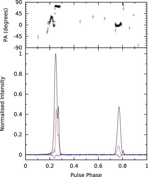
PSR B1937+21 coherently added LEAP profile from observations made on 2014 May 22 (MJD 56799), with the polarization position angles displayed in the top panel. The higher- and lower-amplitude peaks are referred to as the main pulse (MP) and interpulse (IP), respectively. The line types indicate the Stokes parameters: total intensity (I, solid black), total linear (L, dashed red), and total circular (V, dotted blue).
PSR B1937+21 is one of the most luminous MSPs discovered to date, and is included in all currently ongoing pulsar timing arrays (Desvignes et al. 2016; Reardon et al. 2016; Verbiest et al. 2016; Arzoumanian et al. 2018). It is one of the few MSPs that is presently known to exhibit significant timing noise (Kaspi, Taylor & Ryba 1994; Shannon et al. 2013; Caballero et al. 2016), in addition to large variations in dispersion measure (DM) and scattering (Ramachandran et al. 2006; Keith et al. 2013; Levin et al. 2016), all of which impose limitations on the achievable timing precision of the pulsar. It has been shown that the non-GP single-pulse emission from PSR B1937+21 is extremely regular, with no evidence for intrinsic pulse-shape variations over millions of rotations (Jenet, Anderson & Prince 2001), and information gathered from individual rotations of the pulsar may shed light on the nature of the pulsar’s timing noise.
The structure of our paper is as follows: in Section 2, we describe our observations, data reduction, and calibration process. In Section 3, we describe the method we have used to search for GPs in our data set. In Section 4, we present the results of our GP search, and show results of analyses using our GP data set. We discuss our findings in Section 5, and make general concluding comments in Section 6.
2 OBSERVATIONS
Our observations were made using the Large European Array for Pulsars (LEAP); a tied-array telescope comprised of various combinations of five European 100-m class radio telescopes: the Effelsberg Telescope, the Lovell Telescope, the Nançay Radio Telescope (NRT), the Westerbork Synthesis Radio Telescope (WSRT), and the Sardinia Radio Telescope (SRT). Observations with the participating telescopes are made simultaneously and are combined coherently into a tied-array beam, forming a virtual 195-m dish when using all five telescopes. The design of the LEAP experiment is detailed in Bassa et al. (2016).
Monthly observations have been made in LEAP mode since 2012 February, and a summary of the observations analysed here is presented in Table 1. This includes details of the telescopes included in the observing sessions, the central frequency (typically 1396 MHz) and bandwidth (typically 128 MHz), and the observing duration. Differences in bandwidth are due to either the instrumental setup used in the observation or due to data loss, and in all cases the bandwidth uses contiguous sub-bands. Following an observation, the baseband data (raw complex voltages) from the individual telescopes are shipped to Jodrell Bank Observatory (in the case of NRT, data are transferred electronically), where the signals are correlated on a CPU cluster, using a software pipeline detailed in Smits et al. (2017). By correlating the single-telescope data, initially on a nearby calibrator and later on the pulsar itself, time and phase delays are measured between pairs of telescopes, and used to coherently add the single-telescope data to form the LEAP tied-array beam. We define the coherency of a correlated observation as the ratio of the S/N of the combined LEAP profile to the sum of the individual telescope S/Ns. An ideal addition will have a coherency of |$100{{\ \rm per\ cent}}$|, while an incoherent addition (i.e. simply adding the signals without using the phase information of the raw voltages) will have a coherency of |${\sim } N_{\text{tels}}^{-1/2}$|, in cases where the instruments and noise are identical. Prior to 2014 September, data recorded during LEAP observations were archived for future reduction in monthly correlation campaigns. Currently, data are reduced at most two months after an observation, while archived observations are analysed in parallel. As the reduction of the archived data is still ongoing, there are gaps in our reduced data sets prior to 2014 May.
Summary of the 21 LEAP observations of PSR B1937+21 used in this work, and the number of GPs from each observation. Note that two separate observations were made on 2012 September 23, separated by ∼13 min. S/Nprofile refers to the integrated signal-to-noise of the average pulse profile. The ‘Telescopes’ heading refers to the telescopes included in the combined LEAP observation. Telescope code: E: Effelsberg Telescope; J: Jodrell Bank (Lovell Telescope); N: Nançay Radio Telescope; S: Sardinia Radio Telescope; W: Westerbork Synthesis Radio Telescope.
| Date | MJD | Telescopes | fc (MHz) | BW (MHz) | Tobs (s) | S/Nprofile | Coherency (per cent) | NMGP | NIGP | NGP |
|---|---|---|---|---|---|---|---|---|---|---|
| 2012-09-23 (1) | 56193 | EJW | 1412 | 64 | 1240 | 719 | 80 | 125 | 77 | 202 |
| 2012-09-23 (2) | 56193 | EJW | 1412 | 64 | 1020 | 808 | 86 | 124 | 74 | 198 |
| 2013-07-27 | 56500 | EJW | 1404 | 112 | 1800 | 525 | 63 | 138 | 106 | 244 |
| 2013-08-25 | 56529 | EW | 1364 | 64 | 2700 | 1065 | 98 | 278 | 154 | 432 |
| 2014-05-22 | 56799 | ESW | 1396 | 128 | 2760 | 904 | 86 | 168 | 83 | 251 |
| 2014-07-07 | 56845 | EW | 1420 | 80 | 2770 | 435 | 88 | 172 | 84 | 256 |
| 2014-07-27 | 56865 | EW | 1380 | 96 | 2760 | 492 | 97 | 31 | 22 | 53 |
| 2014-08-24 | 56893 | EJNW | 1396 | 128 | 2490 | 852 | 92 | 155 | 75 | 230 |
| 2014-10-15 | 56945 | EJNW | 1380 | 64 | 1470 | 587 | 57 | 139 | 76 | 215 |
| 2015-02-25 | 57078 | EJNW | 1396 | 128 | 2120 | 715 | 76 | 145 | 94 | 239 |
| 2015-03-26 | 57107 | EJNSW | 1396 | 128 | 2510 | 1232 | 82 | 171 | 87 | 258 |
| 2015-04-17 | 57129 | EJNSW | 1396 | 128 | 2510 | 1202 | 80 | 137 | 52 | 189 |
| 2015-06-20 | 57193 | EJW | 1396 | 128 | 2230 | 598 | 100 | 112 | 63 | 175 |
| 2015-07-19 | 57222 | EJS | 1412 | 96 | 2790 | 458 | 67 | 112 | 92 | 204 |
| 2015-09-18 | 57283 | EJN | 1404 | 112 | 2520 | 429 | 78 | 90 | 32 | 122 |
| 2015-10-10 | 57305 | EJ | 1412 | 96 | 2790 | 543 | 86 | 112 | 52 | 164 |
| 2015-11-07 | 57333 | EJS | 1396 | 128 | 2790 | 729 | 99 | 81 | 55 | 136 |
| 2015-12-12 | 57368 | EJNS | 1396 | 128 | 2520 | 755 | 75 | 138 | 55 | 193 |
| 2016-01-09 | 57396 | EJNS | 1396 | 128 | 2520 | 1122 | 83 | 154 | 99 | 253 |
| 2016-02-05 | 57423 | EJNS | 1404 | 112 | 2390 | 629 | 75 | 97 | 49 | 146 |
| 2016-04-07 | 57485 | EJNS | 1388 | 80 | 2380 | 924 | 78 | 110 | 48 | 158 |
| Mean | – | – | – | – | 2337 | 709 | 82 | 133 | 70 | 203 |
| Total | – | – | – | – | 49 080 | – | – | 2789 | 1476 | 4265 |
For each observation, the data were polarization-calibrated using baseband data from observations of PSR J1022+1001 and/or PSR B1933+16, made during the same LEAP observing session, with corresponding polarization templates obtained from the European Pulsar Network data base1 (Stairs et al. 1999). An example of a polarization-calibrated coherently added pulse profile is shown in Fig. 1. Our polarization calibration procedure uses a template-matching algorithm, similar to the method developed by van Straten (2006), which we discuss in detail in Bassa et al. (2016). Coherently added baseband data for the combined LEAP observations are saved to tape for future scientific use.
3 GIANT PULSE SEARCH PIPELINE
Our 21 observations recorded a total of 3.1 × 10⁷ rotations of PSR B1937+21 (equivalent to 13.6 h of observations), and each rotation was searched for GPs. The LEAP baseband data are split into 10-s sub-integrations for each 16-MHz sub-band. These files were concatenated in time and frequency to obtain a single file per observation. During the search, the frequency channels were summed, and both polarizations were summed in quadrature in each rotation. The DM used for coherent dedispersion was chosen using an initial value derived from multifrequency observations of PSR B1937+21 using the Lovell Telescope at 1532 MHz and the Jodrell Bank 42-ft telescope at 610 MHz (Fig. 2). This value was then used to dedisperse data from the first few minutes of the observation, while high S/N (>15σ) GP candidates were searched for (full details of the search follow this paragraph). These initial candidates were then used to recalibrate the DM by finding the values that minimized the pulse width of each of these GPs, and taking the final DM as the mean, and the RMS of the values as the uncertainty. Errors in the DM used to dedisperse the observation can smear out the signal, and lead to a decreased sensitivity to GPs. However, in the case where the full 128 MHz bandwidth is used, we calculate a maximum smearing of |${\sim }0.4\, {}\, \mu {\rm s}$| for a DM error of 0.001 cm−3 pc (i.e. similar to the maximum uncertainty of our DM values used for folding), which does not significantly impact our sensitivity. We note that although we have used the same DM value to dedisperse both the MGPs and IGPs, the true quantity may not be consistent between GPs from each component, which potentially include different contributions from the magnetosphere (Hankins & Eilek 2007). The full search was then performed on the entire observation, which was coherently dedispersed with the optimized DM using dspsr2 (van Straten & Bailes 2011).
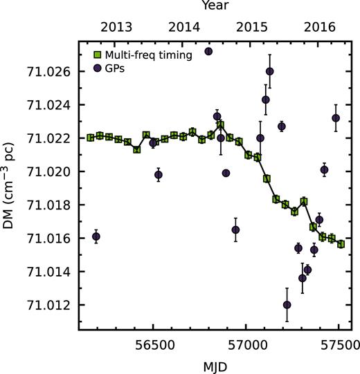
Measured DMs for PSR B1937+21 from multifrequency timing (yellow squares, dashed line) used as the initial guess for the value used in the dedispersion process, and the mean DM measured from GPs from each observation (purple circles). The initial DMs were derived by fitting for DM over 50-d windows in a data set composed of TOAs from the Lovell Telescope’s ROACH backend at a centre frequency of 1532 MHz with 400 MHz of bandwidth, and from the Jodrell Bank 42-ft telescope’s COBRA2 backend at a centre frequency of 610 MHz, with 10 MHz of bandwidth. The 42-ft telescope data are obtained almost daily, and the Lovell Telescope data approximately every 1–2 weeks.
Our DM values obtained from minimizing the pulse width of bright GPs (described above) differ from those obtained from the multifrequency timing (Fig. 2). This may indicate that the DM value that best-optimized our GP search over a small 64 to 128 MHz bandwidth does not optimally describe the DM for observations at widely separated observing frequencies, or that there is a frequency-dependence of the GP structure that contaminates the DM measurement. Scattering and scintillation were not accounted for when choosing the optimal DM. These effects can also cause a frequency-dependent broadening of the pulse and therefore contaminate the DM measurement, but the magnitude is not sufficient to significantly alter measured DMs at our observing frequencies and over our small bandwidth. The DM values obtained via both techniques are in agreement with that of Popov & Stappers (2003) (71.025 cm−3 pc), and the portion of the data set that overlaps with measurements made using the European Pulsar Timing Array data release 1.0 (∼71.02 cm−3 pc; Desvignes et al. 2016), but are consistently lower than those of Cognard et al. (1995) (71.041 cm−3 pc) and Soglasnov et al. (2004) (71.036 ± 0.004 cm−3 pc), which is expected, given the large known DM variations in this pulsar.
The entire data set was divided into single pulses, each with 8192 phase bins and a time resolution of ∼47 ns. This slightly oversampled the data, which has an intrinsic resolution of 62.5 ns, based on the 16 MHz-wide bands. As scattering reduces this peak S/N of pulses, each rotation was searched for pulses that exceeded an S/N threshold of 7σ at three time resolutions of approximately 47, 95, and 190 ns, corresponding to the initial resolution, and downsampling by factors of two and four, respectively, to ensure that scattered GPs were not missed. This also ensured that the diminished signal at high time resolutions did not cause GPs with low flux densities or sub-pulse structure to be missed. Candidates were further selected by generating an intensity versus phase plot from each rotation, and excluding rotations with a peak intensity that occurred outside of a pulse phase window of width 0.06, centred on the peak of the intensity versus phase distribution. This final set of candidates was then inspected by eye, using total-intensity versus pulse phase and frequency channel versus pulse phase plots, to ensure that the signal was not narrow-band RFI (i.e. located in a single band), and that false positives from time-varying broadband RFI were removed.
4 RESULTS
4.1 Giant pulses
Our search yielded 2789 MGPs and 1476 IGPs, for a total of 4265 GPs, which is the largest sample of GPs ever gathered for PSR B1937+21. Our sample has a mean MGP:IGP ratio of 65:35, which is consistent with the findings of Soglasnov et al. (2004), who observed an MGP:IGP ratio of 61:39 for a GP sample size of 309, from a 39-min observation in 1999 May. The mean GP occurrence rate across all of our observations was 205 h−1 for MGPs, and 108 h−1 for IGPs, for a total of 313 h−1. This is lower than the rate of 475 h−1 found by Soglasnov et al. (2004), although we note that there appears to be intrinsic variability in the emission rate, with the rate varying by approximately an order of magnitude across all our observations (from 69 to 699 h−1).
We observe no correlation between integrated pulse profile S/N and number of observed GPs (Fig. 3), which indicates that the variation in emission rate is intrinsic, rather than related to diffractive interstellar scintillation, and that our detection rate is very close to the emission rate at our sensitivities. The number of GPs from each observation is summarized in Table 1. As expected following Kinkhabwala & Thorsett (2000), the GP emission was found to occur in narrow phase windows (much narrower than those used for our candidate selection) located at the trailing edges of the regular emission regions, with the MGP trailing the MP peak by |${\sim }{58}\, \mu {\rm s}$|, and the IGP trailing the IP peak by |${\sim }{64}\, \mu {\rm s}$| (Fig. 4).
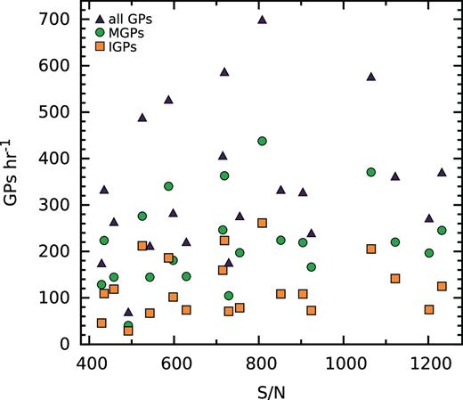
Number of GPs versus integrated profile S/N for the corresponding observation. There is no consistent correlation between the two quantities, indicating that the number of GPs is not S/N limited. IGP: orange squares, MGP: green circles, total GPs: purple triangles.
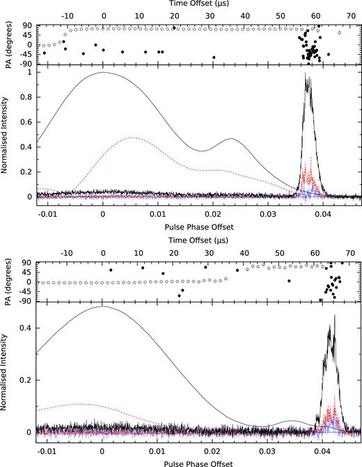
Pulse intensity as a function of pulse phase of the regular emission using 1024 phase bins (centred at 0) and the GP emission using 8192 phase bins, averaged over all 21 observations, with the polarization position angles displayed in the top panels for the regular emission (open circles) and the GP emission (closed circles). The profiles are normalized so that the peak MP and MGP fluxes are unity, and the profiles are rotated so that the peaks of the MP and IP are centred at zero phase. The peak of the MGP trails the peak of the MP by approximately 58 |$\mu$|s (above) and the peak of the IGP trails the peak of the IP by approximately 64 |$\mu$|s (below). In both plots, a small contribution from the normal emission is visible in the GP data, indicating that normal emission occurs simultaneously with GP emission. The line types indicate the Stokes parameters: total intensity (I, solid, black), total linear (L, dashed, red), and total circular (V, dotted, blue).
We note that emission at the phase of the regular average pulse profile is clearly visible in the total GP profile (Fig. 4), which demonstrates that regular emission occurs simultaneously with GP emission. As the GP emission regions are located at the edge of the regular emission regions, and a ‘bump’ in the regular IP emission is coincident with the location of the IGP emission phase, the GP contribution to the regular average pulse profile was investigated. After scaling the total GP profile relative to the average pulse profile by a factor (Nrotations − NGP)−1/2, it was found that the IGP contribution to the flux ratio at the phase of the IP ‘bump’ is ∼0.03, and therefore negligible. Further investigation will be required to determine whether there is a long tail of ‘weak’ GPs that are contributing to the flux at this phase, or if the ‘bump’ is simply a feature of the underlying non-GP emission at this phase. We observe that in the case of high-S/N GPs, resolvable low-intensity emission precedes the leading edge of the main peaks (Fig. 5), which indicates that GP emission in PSR B1937+21 does not occur in a single short-duration burst, but in a manner similar to the ‘nanoshots’ observed in GP emission from the Crab Pulsar (Hankins et al. 2003; Hankins & Eilek 2007).
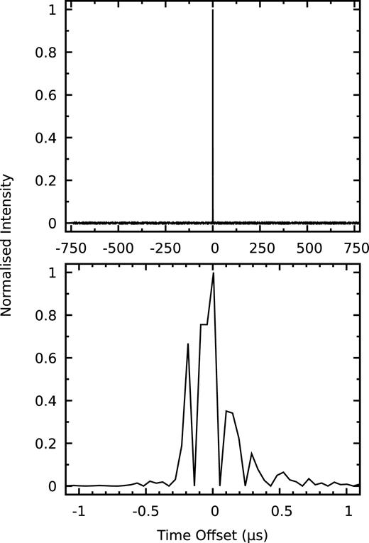
Total-intensity profile of the brightest GP observed in our search. The observation was made on 2014 May 22 (MJD 56799), at a time resolution of ∼47 ns. The integrated signal-to-noise ratio of the pulse is 1988, and the pulse energy is 492 Jy |$\mu$|s. The upper plot shows the full pulse phase, and the lower plot is zoomed in to 0.0014 of the pulse phase (2.2 |$\mu$|s). The effect of scattering on this pulse is very small, with a measured scattering time-scale τsc = 128 ± 8 ns and a pulse width at |$1{{\ \rm per\ cent}}$| of the maximum of |${\sim }{1.5}\, \mu {\rm s}$|.
4.2 Flux calibration
4.3 Giant pulse energy distributions
We plot the cumulative pulse energy distributions of the GPs in our sample in Fig. 6, and observe the expected power-law distribution for high pulse energies. The pulse energy distribution turns over at low energies of ≲2 Jy |$\mu$|s, which is expected due to the finite number of GPs emitted, and as not every rotation contains a GP. While the pulse energies of the IGP distribution are well-modelled with a single power law, we find that the MGP and all-GP distributions are better-modelled with a broken power law, with pulse energies ≳7 Jy |$\mu$|s following a flatter distribution in a similar way to high-energy GPs from the Crab Pulsar (Popov & Stappers 2007). We do not observe any pulse-width-dependent variation in the pulse energy at which the power-law break occurs (Fig. 7), in contrast to that observed in the pulse energy distribution of the Crab Pulsar by Popov & Stappers (2007). The power-law indices we measure are summarized in Table 2, and differ from those reported by Soglasnov et al. (2004) and Cognard et al. (1996), which are α = −1.40 ± 0.01 and α = −1.8 ± 0.1, respectively, for the all-GP distribution. We note that these values were determined using sample sizes approximately one order of magnitude lower than our sample size, and that somewhat different observing frequencies were used. We note also that the power-law indices for the distributions of our individual observations vary significantly, ranging from α = −1.4 ± 0.1 to α = −5.8 ± 0.4 for the all-GP distributions. Drawing random MGPs and IGPs from our distribution, to form sample sizes equal to that of Soglasnov et al. (2004) (309 GPs), we find a mean all-GP power-law index of α = −3.9 ± 0.1 after 1000 trials.
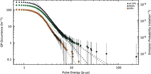
Cumulative occurrence rates and emission probabilities for GPs exceeding a given pulse energy, binned in intervals of 0.1 Jy |$\mu$|s. The pulse energies of the MGPs (green circles), IGPs (orange squares), and all GPs (purple triangles) are plotted separately, with counting errors assigned as the standard error for a Poisson process. The MGP and all-GP distributions clearly exhibit a broken power law for GPs exceeding pulse energies of ∼7 Jy |$\mu$|s. A broken power law is not visible in the IGP distribution, possibly due to the lower number of IGPs exceeding this pulse energy. The dashed lines are the best-fitting power laws for pulse energies greater than the flattened low-energy regime, whose indices are listed in Table 2.
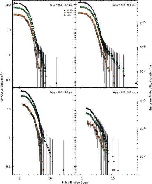
As Fig. 6, for GP pulse energies at a given full-width at half-maximum (W50). The break in the power law occurs at pulse energies of ≳7 Jy |$\mu$|s for the |$0.2\, {}\, \mu {\rm s}\lt W_{50}\lt 0.4\, {}\, \mu {\rm s}$|, |$0.4\, {}\, \mu {\rm s}\lt W_{50}\lt 0.6\, {}\, \mu {\rm s}$|, and |$0.6\, {}\, \mu {\rm s}\lt W_{50}\lt 0.8\, {}\, \mu {\rm s}$| distributions, and is not easily distinguishable in the |$0.8\, {}\, \mu {\rm s}\lt W_{50}\lt 1.0\, {}\, \mu {\rm s}$| distribution. The data points are MGPs (green circles), IGPs (orange squares), and all GPs (purple triangles).
Power-law indices (α) for the pulse energy distributions presented in Fig. 6. The power-law regime is obeyed for pulse energies ≳2 Jy |$\mu$|s, below which the distribution is flattened. The IGP distribution is well-described by a single power law, while the MGP and all-GP distributions are better-described by a broken power law, with indices listed here as ‘low’ and ‘high’.
| Data set | Pulse energy (Jy |$\mu$|s) | α |
|---|---|---|
| IGP | ≳2 | −3.99 ± 0.04 |
| MGPlow | ∼2–7 | −3.26 ± 0.03 |
| MGPhigh | ≳7 | −1.81 ± 0.06 |
| GPlow | ∼2–7 | −3.48 ± 0.04 |
| GPhigh | ≳7 | −2.10 ± 0.09 |
| Data set | Pulse energy (Jy |$\mu$|s) | α |
|---|---|---|
| IGP | ≳2 | −3.99 ± 0.04 |
| MGPlow | ∼2–7 | −3.26 ± 0.03 |
| MGPhigh | ≳7 | −1.81 ± 0.06 |
| GPlow | ∼2–7 | −3.48 ± 0.04 |
| GPhigh | ≳7 | −2.10 ± 0.09 |
4.4 Modulation indices
![Modulation indices [m(ϕ), points with error bars] for all MGPs (left-hand panel) and IGPs (right-hand panel), plotted together with the average intensity of the GPs (solid line). The contribution from the regular emission is visible at the leading edge of each profile. While the distributions appear to be approximately Gaussian, there is significantly more variation in the modulation indices around the centre of the profile (Δm(ϕ) ∼ 0.5) when compared to the edges of the profile, in contrast to the regularity of non-GP single-pulse emission reported by Jenet et al. (2001).](https://oup.silverchair-cdn.com/oup/backfile/Content_public/Journal/mnras/483/4/10.1093_mnras_sty3058/1/m_sty3058fig8.jpeg?Expires=1750302243&Signature=HCH60vOePTGy1mFFkHGh1X-KWdprRJDhr~7J10XXrNyrg2LPsvuM-MoKo~5SFCnNc1cf3cZX3VpHHX5B2v3PJyg6i0KdeJEZa3T70pMAjUkrV-NhOVe1-cwBYVBx7AlEJc5qXLb2DAAslTjXb-Ftqm9Zhw4CrkX~V7CjJlcxgBRq2SVz78yeBD-HT3SzPAavqC9FmvSu~4WvgzqhLKd18D5dWLy-gctV54NoHGlY4dhuHgBbTZ-TuM2wo3elqdIaaPdsyT7KQRdmLfBjpwZGw4dapPk6P7KE7~KEqXaJBHVQUf-7dhZBvfjUfezzz-0BYt43WyMEF5BCweCIWEzwJg__&Key-Pair-Id=APKAIE5G5CRDK6RD3PGA)
Modulation indices [m(ϕ), points with error bars] for all MGPs (left-hand panel) and IGPs (right-hand panel), plotted together with the average intensity of the GPs (solid line). The contribution from the regular emission is visible at the leading edge of each profile. While the distributions appear to be approximately Gaussian, there is significantly more variation in the modulation indices around the centre of the profile (Δm(ϕ) ∼ 0.5) when compared to the edges of the profile, in contrast to the regularity of non-GP single-pulse emission reported by Jenet et al. (2001).
4.5 Scattering and DM variations
The measured DM of PSR B1937+21 is known to fluctuate significantly between observations (Cordes et al. 1990; Ramachandran et al. 2006), and it has been suggested that scatter-broadening is the only cause of variations in the observed pulse shape of the regular emission (Jenet et al. 2001). We observe a wide distribution of GP widths (Fig. 9), similar to the findings of Karuppusamy, Stappers & van Straten (2010) of the GP width variations due to large changes in scattering in the Crab Pulsar. Our data set allowed us to make many separate scattering measurements over the course of each observation, using individual GPs. As observed GPs are often composed of several individual peaks, we smooth the pulse shape using a Savitzky–Golay filter (Savitzky & Golay 1964), enabling the smoothed pulse to be approximated as an exponentially modified Gaussian (Fig. 10, and see McKinnon 2014; McKee et al. 2018). The scattering time-scales measured using an exponentially modified Gaussian fit to the smoothed IGP and MGP for each observation are in good agreement (Fig. 11).
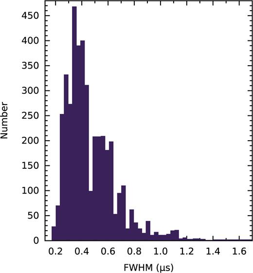
Distribution of observed GP pulse widths, measured at the half-maximum, after fitting an exponentially modified Gaussian function to GPs that were smoothed with a Savitzky–Golay filter. The distribution has a clear peak at |${0.35}\, \mu {\rm s}$|, followed by a decay to more rare instances of broader pulse widths.
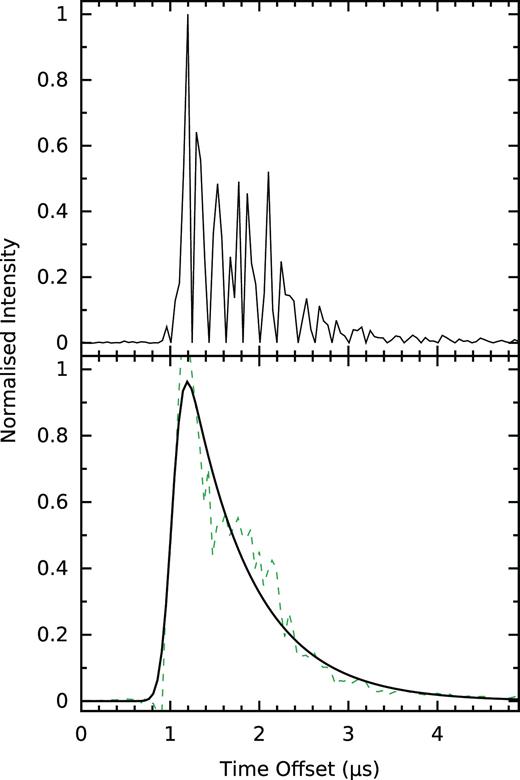
Example of scattering observed in a bright GP. The profile (above) has a pulse energy of 242 Jy |$\mu$|s (integrated S/N = 959) and a clear exponential scattering tail. The scattering time-scale is measured (below) by fitting an exponentially modified Gaussian function (solid line) to the observed GP (dashed line), after smoothing with a Savitzky–Golay filter (see text), which mitigates the effect of the ‘spiky’ emission on the fitting process. The scattering time-scale in this profile is measured to be τsc = 676 ± 32 ns. The separation of the visible quasi-periodic micro pulses is about 200 ns, which is exemplary for the value determined for the larger sample of GPs of 249 ± 197 ns (see Section 5.1 for details).
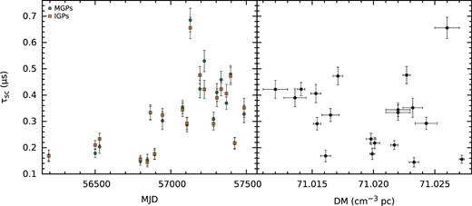
Left-hand panel: Mean GP scattering time-scales for each of our observations, measured using exponentially modified Gaussian fits to each MGP (green circles) and IGP (orange squares; see text for details). The measurements from each GP component are in good agreement and show significant variation across our observations. Right-hand panel: Mean scattering versus DM for each of our observations. The two quantities do not appear to be correlated, in contrast to the strong correlation observed in pulsars such as the Crab.
The distribution of our measured scattering time-scales presented in Fig. 12 is in good agreement with those obtained by Cordes et al. (1990) at observing frequencies of 430 MHz, assuming that scattering scales with observing frequency as τsc ∝ f−4.4 (the frequency scaling of scattering time-scales in PSR B1937+21 between 400 MHz and 2 GHz has been found by Kondratiev et al. 2007 to be consistent with the expected f−4.4 scaling). The distribution has a clear peak at a time-scale |$\tau _{\text{sc}}={0.15}\, \mu {\rm s}$|, and |${\sim }64{{\ \rm per\ cent}}$| of pulses have scattering time-scales |$\lt {0.35}\, \mu {\rm s}$|. As expected from the findings of Ramachandran et al. (2006), the mean scattering time-scale was found to vary significantly between observations (Fig. 11), and instances of very high scattering were found to skew the mean scattering time-scales for the observations.
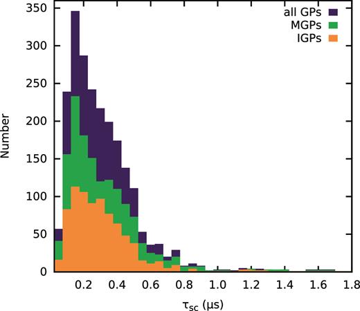
Scattering time-scales measured from the exponentially modified Gaussian fit to the smoothed GPs. The measured values are binned at intervals of 50 ns, and the most common time-scale is |${0.15}\, \mu {\rm s}$|. The time resolution of our observations does not allow scattering time-scales <60 ns to be identified.
We find no correlation between the mean scattering time-scale and DM (Fig. 11) measured in each of our observations. This is in contrast to the strong correlation observed between scattering time-scales and DM seen in the Crab Pulsar (Kuzmin et al. 2008; McKee et al. 2018). We also find no correlation between the mean scattering time-scale and DM, and the normal pulse time of arrival (TOA) error (Fig. 13). This indicates that unmodelled variations in these quantities do not limit the precision of our TOAs for PSR B1937+21, at our observing frequencies and sensitivity.
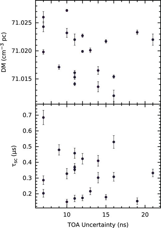
Mean scattering time-scales measured from the GPs (below), and the mean DM measured from GPs (above) versus TOA uncertainty measured using the regular pulse profile. In both plots, the two quantities do not appear to be correlated.
4.6 Giant pulse polarization
While the emission from the average pulse profile of PSR B1937+21 is approximately |$50{{\ \rm per\ cent}}$| linearly polarized and has very little circular polarization (Fig. 1), GPs from PSR B1937+21 are often observed to be highly polarized, with some bright GPs displaying almost |$100{{\ \rm per\ cent}}$| circular polarization (Cognard et al. 1996; Soglasnov et al. 2004). The GPs in our sample are not rotation measure corrected. However, we estimate that the error introduced to the position angle (PA) between the top and bottom of our maximum bandwidth is ∼0.07 rad, for a rotation measure of 8.3 rad m−2 (Dai et al. 2015), which will not significantly alter the polarization properties. The polarization profile of the GPs averaged over all 21 observations is different to that of the averaged regular pulse profile (Fig. 4), implying that the polarized-emission statistics of GPs are different to those of the regular individual pulses. There are some difficulties in measuring polarized emission at time resolutions approximately equal to the Nyquist sampling rate, as is the case for our data set, or in cases where the sampling resolution is approximately equal to the scattering time-scale. In these cases, unresolved emission can appear to be |$100{{\ \rm per\ cent}}$| polarized in each sample (Cordes 1976; van Straten 2009), although in our analysis we average over multiple samples and frequency channels, and thus our polarization measurements are not impacted by our choice of sampling resolution. In Fig. 14, we plot histograms of the observed fractions of linear and circular polarization from our GPs. We find that the GPs in our data set tend to be highly linearly polarized, and we observe that while there are instances of almost entirely polarized GPs, these are comparatively rare. Of the GPs in our data set, |$1.1{{\ \rm per\ cent}}$| of MGPs and |$0.6{{\ \rm per\ cent}}$| of IGPs display |$\gt 90{{\ \rm per\ cent}}$| circular polarization, while |$6.0{{\ \rm per\ cent}}$| of MGPs and |$3.9{{\ \rm per\ cent}}$| of IGPs are |$\gt 90{{\ \rm per\ cent}}$| linearly polarized. We find that while the histograms of fractional circular polarization are similar for MGPs and IGPs, the fractional linear polarization histograms are different for the highly polarized MGPs and IGPs, with a higher portion of MGPs displaying |$\gt 50{{\ \rm per\ cent}}$| linear polarization. We find no evidence for phase-dependence of polarized emission, nor are there significant differences between the IGP and MGP polarization fraction distributions (Fig. 15), in agreement with the findings of Zhuravlev et al. (2013). We also find no correlation between GP pulse energy and fractional polarization or GP width.
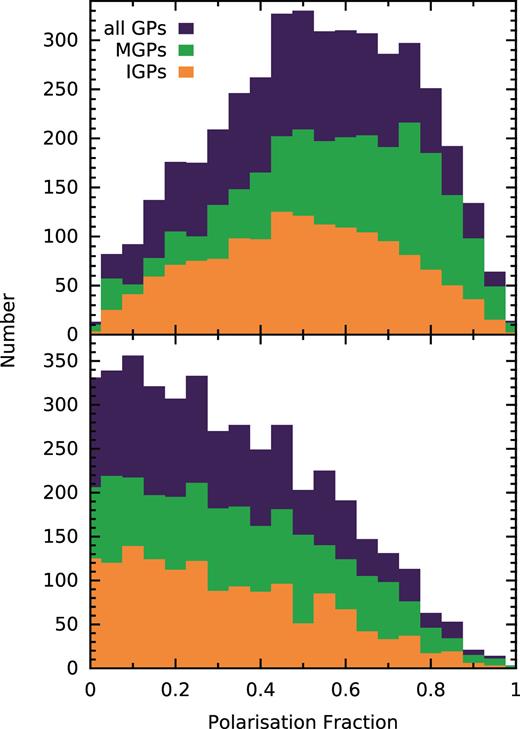
Histograms of the fractions of linear (L/I, above) and circular (|V|/I, below) polarization of the MGPs (green), IGPs (orange), and all GPs (purple) in our data set.
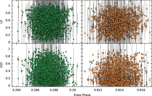
Distributions of fractional linear (L/I, top row) and circular (|V|/I, bottom row) polarization of MGPs (left-hand column, green) and IGPs (right-hand column, orange), according to their phase location relative to the peak MP total-intensity emission (centred at a phase of 0.25). The fractional polarization of the emission does not appear to be dependent on the location within the emission phase, nor are there significant differences between the MGP and IGP distributions.
5 DISCUSSION
5.1 Giant pulse emission properties
The phase window in which GPs occur may allow the properties of the GP emission region to be constrained. For example, a model by Lyutikov (2007) describes GPs in the Crab Pulsar as originating from the last closed field lines, in contrast to the regular emission, which originates from the open field lines. In the Lyutikov (2007) model, the observer angle to this section of the field lines must fall within a narrow (∼10−3 rad) range, implying that the rarity of known GP-emitting pulsars is due to the low probability that this specific alignment will occur, and could explain the narrow phase region in which GPs are observed (Fig. 4).
Pulsars for which bright single-pulse emission has been detected, and the corresponding magnetic field strength at the light cylinder (BLC). The ‘rank’ column refers to the position of the pulsar when sorting the 2109 pulsars for which this property is currently listed in the ATNF Pulsar Catalogue by their magnetic field strengths at the light cylinder. Pulsars that are classified as GP emitters have BLC > 105 G (see text).
| Name | BLC (G) | Rank | Reference |
|---|---|---|---|
| B1937+21 (J1939+2134) | 1.0 × 10⁶ | 2 | Wolszczan et al. (1984), Cognard et al. (1996) |
| B0531+21 (J0534+2200) | 9.6 × 10⁵ | 3 | Staelin & Reifenstein (1968) |
| B1821 − 24A (J1824 − 2452A) | 7.4 × 10⁵ | 4 | Romani & Johnston (2001) |
| B1957+20 (J1959+2048) | 3.8 × 10⁵ | 6 | Joshi et al. (2004) |
| B0540 − 69 (J0540 − 6916) | 3.6 × 10⁵ | 7 | Johnston & Romani (2003) |
| J0218+4232 | 3.2 × 10⁵ | 9 | Joshi et al. (2004) |
| B1820 − 30A (J1823 − 3021A) | 2.5 × 10⁵ | 16 | Knight et al. (2005) |
| B0656+14 (J0659+1414) | 770 | 437 | Kuzmin & Ershov (2006) |
| B0950+08 (J0953+0755) | 140 | 790 | Singal (2001), Smirnova (2012) |
| J1752+2359 | 71 | 1007 | Ershov & Kuzmin (2005) |
| B0529 − 66 (J0529 − 6652) | 39 | 1183 | Crawford et al. (2013) |
| B0031 − 07 (J0034 − 0721) | 7.0 | 1694 | Kuzmin, Ershov & Losovsky (2004) |
| B1112+50 (J1115+5030) | 4.2 | 1832 | Ershov & Kuzmin (2003) |
| B1237+25 (J1239+2453) | 4.1 | 1843 | Kazantsev & Potapov (2017) |
As mentioned earlier, GPs are believed to be a radio component of the high-energy emission, and they may be expected to originate from a different altitude or location in the magnetosphere to that of the regular radio emission. A widely used method for measuring the emission height of different components of the pulsar beam is given by Blaskiewicz, Cordes & Wasserman (1991). In their model, the phase at which the steepest gradient of the polarization PA occurs is interpreted as the closest approach of the line of sight to the pulsar’s magnetic pole, and the emission height is calculated using the phase difference between this fiducial point and the peak intensity of the pulse profile. For this method to be used, the precise polarization PA morphology is required. However, GPs from PSR B1937+21 are observed to occur at the edge of the regular emission region i.e. widely separated from the magnetic pole, and where the polarization PA is found to flatten. Additionally, scattering by the interstellar medium, which is known to be relatively high in PSR B1937+21 (e.g. Levin et al. 2016), also flattens the polarization PA (Li & Han 2003). These two effects give rise to a featureless GP polarization PA, making the Blaskiewicz et al. (1991) model difficult to apply to measuring the GP emission height. The emission height of GPs has also been measured (e.g. Karuppusamy, Stappers & Serylak 2011) using a model by Kardashev et al. (1982), where the frequency-dependence of the component separation is used to determine the difference in emission heights. However, as MSP emission heights exhibit very little variation with frequency (Kramer et al. 1999), a study like this would require a much wider bandwidth than our maximum of 128 MHz, or simultaneous multifrequency observations of GPs.
The GPs in our data set vary significantly in shape and intensity over the observing bandwidth throughout each observation. In Figs 16 and 17, we plot the 22 highest-S/N GPs from the observation from 2015 November 7 (MJD 57333, chosen due to its high coherency use of the full 128 MHz bandwidth), separated into eight 16-MHz sub-bands. We observe that both the MGPs and IGPs are composed of multiple components with widths smaller than our time resolution, and that these components vary in relative intensity with frequency and time of emission. This variation in component intensity with frequency is not coincident with the scintillation at the time of emission, and must therefore be an intrinsic property of the emission. When comparing the sub-band S/N for GPs with the regular emission (Fig. 18), there is a slight correlation, which may be expected if in this case scintillation is affecting the brightness of the GPs, as noted by Popov & Stappers (2003). However, very bright emission is observed in single bands of most GPs, which cannot be accounted for by scintillation alone, and indicates that there is intrinsic variability in the GP emission spectra. Additionally, the typical scintillation bandwidth, estimated from the typical scattering time-scales presented in Fig. 12, is ∼7 MHz, or less than half of the width of the sub-bands we have used.

Comparison of frequency-resolved GP shapes with the full-observation dynamic spectrum, using data from 2015 November 7 (MJD 57333). Above: Total-intensity MGPs, plotted by sub-band. Each GP is normalized by the highest intensity across all frequencies, and centred on the phase of the highest-intensity bin in the frequency-averaged GP profile. Only GPs with S/N > 8σ are plotted to preserve clarity. Below: Dynamic spectrum of the total observation, averaged over 1-min sub-integrations, and normalized by the highest intensity across the total observation. The nulls at the band edges are due to masking of instrumental artefacts. The dashed lines correspond to the GPs in the above panel.
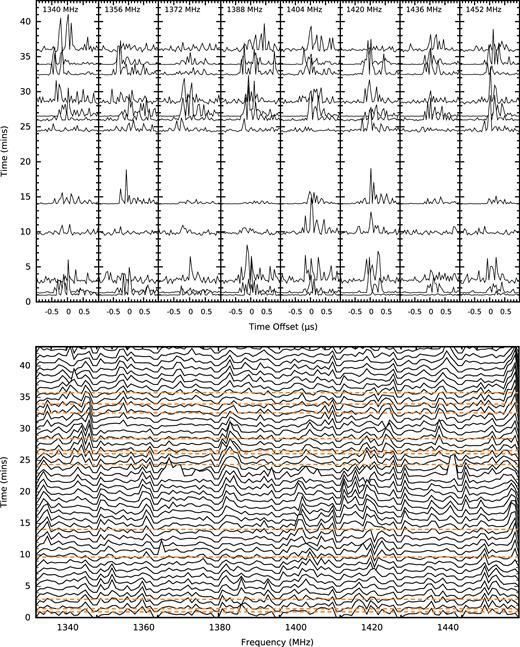
As Fig. 16 for the IGPs.
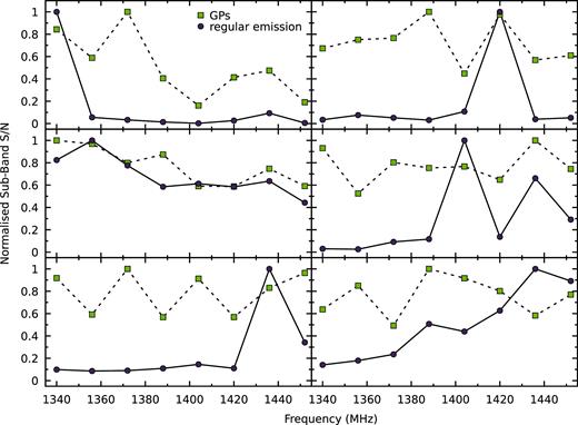
Comparison of sub-band S/N for selected bright GPs (purple circles, dashed lines) and the regular emission integrated over 10īs and coincident with the GP (yellow squares, solid lines). While there may be some correlation between the GP and non-GP spectra, there is underlying intrinsic frequency dependence on the brightness of the GP emission.
While the pulse shapes of the MGPs and IGPs do not appear to be correlated, there does appear to be a correlation on short time-scales between GPs from the same emission region (Figs 16 and 17). The time-scale of the GP microstructure was investigated, following the approach used by Kramer et al. (2002) for regular emission, where periodicities in the sub-pulse emission are identified as peaks in the autocorrelation of individual GPs. Through this, the mean time-scale of the separation between GP micropulses was found to be 249 ± 197 ns, which follows the trend presented in Kramer et al. (2002), where the microstructure time-scale is related to the pulsar spin period and is described by a power law (Fig. 19). The continuation of the scaling to a short-period pulsar suggests that GP emission could be composed of rotating mini-beams, which are likely the fundamental entities of emission, similar to the nanoshots observed in GP emission from the Crab Pulsar (Hankins et al. 2003; Hankins & Eilek 2007). As the PSR B1937+21 GP beam width is very much consistent with the scaling with period, we interpret this as evidence for beaming as a natural explanation for the observed short-duration of GPs.

5.2 Giant pulse emission rates
Our large sample of GPs allows us to calculate the GP emission rate statistics. The statistics have applications in studies of the emission physics of GPs, and information about the typical wait time between GPs is useful in scintillometry, where GPs occurring within a time less than the decorrelation time-scale are required to find the interstellar medium transfer function (e.g. Main et al. 2017). Our observed emission rate from a large sample, and spanning a large number of widely separated observations confirms that GPs from PSR B1937+21 occur very rarely. If we assume that the rates we calculate above are representative of the true emission rate, and that GPs are independent events, the probability of an IGP being emitted in a given rotation is Pr(IGP) = 4.7 × 10⁻⁵, while an MGP has Pr(MGP) = 8.9 × 10⁻⁵, and a GP from either emission region has Pr(GP) = 1.4 × 10⁻⁴. We did not observe an MGP and IGP in the same rotation, although this is not surprising as the probability of observing a so-called ‘double giant pulse’ in our data set is only |${\sim }21{{\ \rm per\ cent}}$|, using the values above. For a |$95{{\ \rm per\ cent}}$| probability of observing a double giant pulse, 1.4 × 10⁸ rotations would be required, approximately 4.5 times more than our data set.
It has been proposed that GPs result from a self-organized criticality process (Bak, Tang & Wiesenfeld 1988), where the underlying emission mechanism reaches some critical point, causing an ‘avalanche process’ that results in GP emission (e.g. Cairns 2004; Melatos, Peralta & Wyithe 2008). Assuming this to be true, and that GP emissions from both components are independent events, the distribution of separations is expected to follow a Poisson probability distribution (Lundgren et al. 1995), which gives rise to an exponentially decreasing time between pulses from the most likely time separation. We confirm that the expected distribution is followed for GPs from PSR B1937+21, by plotting the IGP time separations and MGP time separations separately, binned in intervals of 100 rotations, and fitting an exponential function N(t) = N0exp (−λt) to the distribution (Fig. 20). This provides a good fit, with decay constants λMGP = 1.28 ± 0.01 × 10⁻⁴ and λIGP = 7.3 ± 0.1 × 10⁻⁵. From the exponential function, the mean separation between successive GPs can be estimated from the inverse of the decay constant as |$\lambda _{\text{MGP}}^{-1}=7813\pm 61$| rotations (12.2 ± 0.1 s) and |$\lambda _{\text{IGP}}^{-1}=13699\pm 188$| rotations (21.4 ± 0.3 s).
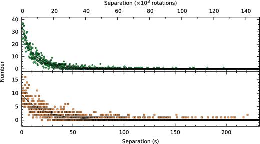
Distribution of time intervals between successive MGPs (above, green circles) and IGPs (below, orange squares) for our entire data set, and the best-fitting exponential functions to these distributions (solid lines). The distributions are well-described by an exponential decay, where the decay constant implies a mean GP rate of one MGP every 7813 ± 61 rotations (12.2 ± 0.1 s) and one IGP every 13ī699 ± 188 rotations (21.4 ± 0.3 s).
5.3 Fast radio bursts and undiscovered pulsars
It has been proposed that fast radio bursts (FRBs) could be explained by the very brightest GPs from pulsars located at cosmological distances (e.g. Cordes & Wasserman 2016). The lowest-inferred luminosity distance estimate of an FRB listed in the Fast Radio Burst Catalogue4 (Petroff et al. 2016) is ∼0.54 Gpc (FRB 170827; Farah et al. 2017). The occurrence rate for FRBs at 1400 MHz with pulse energies of 130–1500 Jy |$\mu$|s has been estimated to be |$7^{+5}_{-3}\times 10^{3}$| events sky−1 d−1 (Champion et al. 2016). From the power-law index we measure for the high-energy GPs, and assuming a distance to PSR B1937+21 of 3.27 kpc (Desvignes et al. 2016), the wait time for a 130 Jy |$\mu$|s GP from a PSR B1937+21-like pulsar at 0.5 Gpc is 6.2 × 10²³ h, or 7.1 × 10¹⁹ yr. For the lower limit of the Champion et al. (2016) rate to be explained by a population of GP-emitting PSR B1937+21-like pulsars, a population of ∼1026 would be required, which appears to rule out PSR B1937+21-like pulsars as the cause of the observed occurrence rate of FRBs. For this rate to be achieved, additional flattening of the pulse energy distribution at high pulse energies, as is the case with so-called ‘super-giant pulses’ observed in the Crab Pulsar (Cordes et al. 2004), would be required.
An undiscovered population of pulsars is thought to exist in the Galactic Centre (GC; distance ∼8.3 kpc; Gillessen et al. 2009, Wharton et al. 2012) of which it is estimated ∼104 are detectable from the Earth (i.e. those whose beams cross the line of sight from the Earth; Rajwade, Lorimer & Anderson 2017). Detection of this population may be possible via single-pulse searches for the GP-emitting pulsars. Assuming the single-pulse detection limit of 130 Jy |$\mu$|s from Champion et al. (2016) used above, the wait time for a GP from a PSR B1937+21-like pulsar at the distance of the GC is 5376 h. If the fraction of GP emitters in the GC is the same as that of the known pulsar population (∼0.005, Table 3), and their pulse energies all follow a PSR B1937+21-like power law, the wait time for a detectable GP from the GC is 108 h. However, in-depth searches for GPs from known pulsars have not been made, and in fact the true fraction of GP emitters is likely to be much higher.
5.4 Timing of giant pulses
GPs are characterized by their extremely short duration compared to the width of the average pulse profile (typically a factor of 100 narrower in the case of PSR B1937+21, with a GP duty cycle of δ ∼ 0.001). As small duty cycles are related to TOA error by σTOA ∝ δ3/2, GPs offer the opportunity to measure TOAs to much higher precision than is possible with the average pulse profile. This also has the advantage of providing many timing measurements in a given observation, allowing small-scale timing effects to be better isolated. The prospect of improving the PSR B1937+21 timing precision is particularly interesting, as it is one of two MSPs, along with PSR B1821 − 24A (PSR J1824 − 2452A) which is also a GP emitter (Romani & Johnston 2001), for which timing noise is easily measureable (e.g. Cordes & Downs 1985). This limits the timing stability on time-scales greater than a few weeks (Kaspi et al. 1994). As mentioned earlier, the non-GP single-pulse emission from PSR B1937+21 shows no evidence for pulse-shape variations (Jenet et al. 2001), which implies that irregularities in the spin of the pulsar due to e.g. intrinsic spin instabilities or the presence of an asteroid belt (Shannon et al. 2013) are the cause of the observed timing noise. In contrast, other MSPs have been observed to display significant jitter noise through pulse-to-pulse variations (e.g. Liu et al. 2012; Shannon et al. 2014), sub-pulse drifting (e.g. Edwards & Stappers 2003; Liu et al. 2016), or variations in flux density (e.g. Wang, Manchester & Johnston 2007).
To study the timing properties of GPs from PSR B1937+21, TOAs were generated from the polarization- and frequency-averaged profiles of each of the GPs, by using standard timing techniques (e.g. Taylor 1993). To account for the variable pulse shapes exhibited by the GPs (Figs 16 and 17), a noise-free template was made for the MGPs and IGPs separately, based on the highest-S/N in both of these categories. This template was found to describe the GPs well, with a typical TOA error of 3 ns and a maximum TOA error of 63 ns. TOAs were also generated using the average pulse profile of each of the observations, using a noise-free artificial reference template based on the highest-S/N observation of PSR B1937+21 with LEAP. The MGP, IGP, and average pulse profile timing residuals were analysed using an ephemeris derived from that presented in Desvignes et al. (2016), and a constant offset was fit between all three data sets.
Residuals from the average pulse profile TOAs were found to have a weighted RMS consistent with that of 4-yr subsets of the Desvignes et al. (2016) data set. The TOAs from each observation did not necessarily use the same centre frequency (Table 1), and were corrected for DM variations by fixing the value to that found from the multifrequency timing from the Lovell Telescope and the 42-ft telescope (see Section 3). It was found that the DM values used to minimize the GP widths added significant structure to the residuals, mirroring the variation of these values seen in Fig. 2, which indicates that the DM values used to optimize the GP search do not accurately describe the delay seen in the timing data. This may be due to some additional or variable dispersion of GP by the pulsar magnetosphere, as seen in the Crab Pulsar (Hankins & Eilek 2007), or due to frequency evolution of the GP pulse shapes (Figs 16 and 17).
We find that although the TOA errors for the individual GPs used in our timing data set are much lower than those of the average pulse profiles (with the lowest average pulse profile TOA error being 7 ns), the timing precision is not significantly different when using the GPs, with the resulting weighted RMS of the residuals being 28.0, 25.7, and 28.8 |$\mu$|s for the MGP, IGP, and average pulse profile TOAs, respectively, and mean residuals weighted by number of TOAs in an observation of 13.6 ns for the MGPs and 26.2 ns for the IGPs (Fig. 21). Although using GPs to time PSR B1937+21 does not offer a significant improvement in timing precision, more rotationally stable GP-emitting pulsars (e.g. PSR J0218+4232) may still benefit from this approach. The spread of the GP residuals is as expected from the pulse width of the average GP profile, where the rate and amplitude of individual GPs leads to the average GP shape (Fig. 4). Using average GP profiles from each observation, we measure the mean widths of the MGP and IGP distributions to be |$4\pm {1}$| and |$4\pm {2}\, \mu {\rm s}$|, respectively, which are consistent with the values reported by Kinkhabwala & Thorsett (2000).
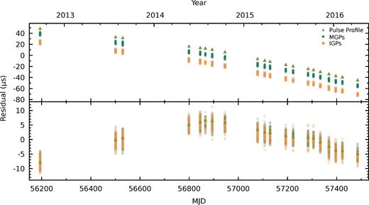
Timing residuals for the average pulse profile (yellow triangles), and GPs (green circles: MGP, orange squares: IGP). Above: Timing residuals using the EPTA data release 1.0 timing model (Desvignes et al. 2016), with the MGP and IGP residuals offset from the average pulse residuals by −10 and −25 |$\mu$|s, respectively, for clarity. The weighted RMS of the residuals, using the EPTA model, is 28.0, 25.7, and 28.8 |$\mu$|s for the MGP, IGP, and average pulse profile data sets, respectively. The weighted RMS of the average-profile residuals is consistent with that of 4-yr subsets of the Desvignes et al. (2016) data set. As expected, the spread of GP residuals is consistent with the width of the folded GP profiles (Fig. 4). Below: Timing residuals aligned using constant phase offsets between the three data sets, with a linear term removed to aid clarity.
6 CONCLUSIONS
We have searched for GPs in baseband data from 13.6 h of observations of PSR B1937+21 with the LEAP telescope, finding a total of 4265 GPs, which is the largest-ever sample of GPs for this pulsar. We do not observe GPs in consecutive rotations, but calculate that this is not surprising, given the size of our data set. By using a modified version of the radiometer equation, we have estimated the pulse energy for each of the GPs, which we have used to comment on the pulse energy distributions and emission rates. We have measured the scattering influence on the pulse shapes of individual GPs and found no correlation between mean scattering time-scale and DM. We find that individual GPs generally have higher fractional polarizations than that of the average pulse profile, and find that there is no phase-dependence of the polarized emission from within the GP emission region. We use the GPs to time PSR B1937+21, and find that although the achievable TOA precision is much higher for GPs than for the average pulse profile, the weighted RMS of the GP timing residuals does not offer a significant improvement over those of the average pulse profile.
We note that the GP emission rate and pulse energy distribution power-law indices vary considerably between observations, as does the structure of individual GPs. These properties are in contrast to the high stability observed in the regular pulse emission (Jenet et al. 2001), and are in agreement with the significant measurement of pulse modulation for the GP pulse stacks (Fig. 8). The difference in these properties between the regular emission and the GP emission, and the fact that we see regular emission and GP emission can occur simultaneously (Fig. 4) supports the hypothesis that GP emission arises from a separate process to that of the regular emission.
ACKNOWLEDGEMENTS
We thank Patrick Weltevrede, Bhaswati Bhattacharyya, Cristina Ilie, Axel Jessner, Robert Wharton, Joris Verbiest, and Aris Noutsos for valuable discussions. This work is supported by the ERC Advanced Grant ‘LEAP’, Grant Agreement Number 227947 (PI M K). The European Pulsar Timing Array (EPTA) is a collaboration between European Institutes, namely ASTRON (NL), INAF/Osservatorio di Cagliari (IT), the Max-Planck-Institut für Radioastronomie (GER), Nançay/Paris Observatory (FRA), The University of Manchester (UK), The University of Birmingham (UK), The University of Cambridge (UK), and The University of Bielefeld (GER), with an aim to provide high-precision pulsar timing to work towards the direct detection of low-frequency gravitational waves. Access to the Lovell Telescope is supported through an STFC consolidated grant. The Effelsberg 100-m telescope is operated by the Max-Planck-Institut für Radioastronomie. The Westerbork Synthesis Radio Telescope is operated by the Netherlands Foundation for Radio Astronomy, ASTRON, with support from NWO. The Nançay Radio Observatory is operated by the Paris Observatory, associated with the French Centre National de la Recherche Scientifique. KJL gratefully acknowledge support from National Basic Research Program of China, 973 Program, 2015CB857101 and NSFC 11373011. KL and RK also gratefully acknowledge support from ERC Synergy Grant ‘BlackHoleCam’, Grant Agreement Number 610058 (PIs: H. Falcke, M K, L. Rezzolla).
