


ABSTRACT
While the evolution of superbubbles driven by clustered supernovae has been studied by numerous authors, the resulting radial momentum yield is uncertain by as much as an order of magnitude depending on the computational methods and assumed properties of the surrounding interstellar medium (ISM). In this work, we study the origin of these discrepancies, and seek to determine the correct momentum budget for a homogeneous ISM. We carry out 3D hydrodynamic and magnetohydrodynamic (MHD) simulations of clustered supernova explosions, using a Lagrangian method and checking for convergence with respect to resolution. We find that the terminal momentum of a shell driven by clustered supernovae is dictated primarily by the mixing rate across the contact discontinuity between the hot and cold phases, and that this energy mixing rate is dominated by numerical diffusion even at the highest resolution we can complete, 0.03 M⊙. Magnetic fields also reduce the mixing rate, so that MHD simulations produce higher momentum yields than HD ones at equal resolution. As a result, we obtain only a lower limit on the momentum yield from clustered supernovae. Combining this with our previous 1D results, which provide an upper limit because they allow almost no mixing across the contact discontinuity, we conclude that the momentum yield per supernova from clustered supernovae in a homogeneous ISM is bounded between 2 × 10⁵ and 3 × 10⁶ M⊙ km s−1. A converged value for the simple homogeneous ISM remains elusive.
1 INTRODUCTION
Feedback from supernovae (SNe) is an important component of understanding the interstellar medium (ISM), galactic winds, and galactic evolution (e.g. McKee & Ostriker 1977; Dekel & Silk 1986; Murray, Quataert & Thompson 2005; Jenkins & Tripp 2011; Kim, Kim & Ostriker 2011; Ostriker & Shetty 2011; Hopkins, Quataert & Murray 2012; Creasey, Theuns & Bower 2013; Dekel & Krumholz 2013; Faucher-Giguère, Quataert & Hopkins 2013; Thompson & Krumholz 2016). Unfortunately, the processes governing the strength of SN feedback operate non-linearly and at small scales. This makes it difficult to include the effects of SNe in analytic models or large galactic simulations without a simplified prescription for SN feedback.
In the past, most investigations of the key factors governing SN feedback strength have focused on single, isolated SNe (e.g. Chevalier 1974; Cioffi, McKee & Bertschinger 1988; Thornton et al. 1998; Iffrig & Hennebelle 2015). In reality, however, core collapse SNe are clustered in space and time: massive stars are born in clusters, and explode after ∼3–40 Myr, before these stars can significantly disperse. The few studies that have looked at the feedback from multiple clustered, interacting SNe have found conflicting results. While some studies have found relatively small changes in the momentum from clustering SNe (Kim & Ostriker 2015; Walch & Naab 2015; Kim, Ostriker & Raileanu 2017), others have found that it could increase the average momentum per SN to 5–10 times greater than the traditional yields for isolated SNe (Keller et al. 2014; Gentry et al. 2017).
It has been suggested that the differences in results for clustered SN simulations could stem from the different levels of mixing in the simulations, from both physical and non-physical sources. Unfortunately, each recent simulation was idealized in significantly different ways, which makes it difficult for us to directly isolate which aspects were the primary drivers of the differences. Our goal in this paper is to identify the causes of the discrepancies between different published results, and resolve whether, when including appropriate physics, clustering does in fact lead to significant changes in the terminal momentum of supernova remnants.
One of the key issues that we investigate is dimensionality and resolution. We found that clustering produces an order of magnitude enhancement in momentum (Gentry et al. 2017), but these results were based on 1D spherically symmetric simulations. Assuming spherical symmetry is potentially misleading because we know of fluid instabilities (such as the Vishniac instabilities and the Rayleigh–Taylor instability) that affect SNR morphologies (Vishniac 1983, 1994; Mac Low & McCray 1988; Mac Low & Norman 1993; Krause et al. 2013; Fierlinger et al. 2016). Even small perturbations can be amplified and noticeably change key properties of SNR evolution. For isolated SN simulations, 1D and 3D simulations do not produce significantly different terminal momenta (e.g. Kim & Ostriker 2015, Martizzi, Faucher-Giguère & Quataert 2015, and Walch & Naab 2015 all find differences of less than 60 per cent between 1D and 3D), but it is worth re-investigating the issue for clustered SNe. It could be that the longer time frame allows the instabilities to grow to have larger effects.
Conversely, our 1D simulations achieved much higher resolution than in any of the 3D simulations found in the literature. We found that the terminal momentum for clustered SNe did not converge until we reached peak resolutions better than 0.1 pc, far higher than the resolutions of published 3D simulations. Moreover, we achieved this convergence only by using pseudo-Lagrangian methods that minimized numerical diffusion across the contact discontinuity at the inner edge of the superbubble, whereas many of the published 3D results are based on Eulerian methods that, for fronts advecting across the grid at high speed, are much more diffusive. Indeed, it is noteworthy that the one published 3D result that finds a significant momentum enhancement from clustering (Keller et al. 2014) uses a Lagrangian method, while all the papers reporting no enhancement are based on Eulerian methods. Clearly, given the conjoined issues of resolution and dimensionality, further investigation is warranted.
Since the suppression and enhancement of mixing is a key unknown for the feedback budget of clustered SNe, we also explore the role of magnetic fields, which may reduce the amount of physical mixing. Our interest in this possibility comes primarily from the example of cold fronts in galaxy clusters, where magnetic fields draped across a shock front have been used to explain the stability of these cold fronts against fluid instabilities (Vikhlinin, Markevitch & Murray 2001; Markevitch & Vikhlinin 2007; although see also Churazov & Inogamov 2004 who show that magnetic fields might not be necessary for stabilizing cold fronts).
In this paper, we first test the effects of bringing our simulations from 1D to 3D and carry out a 3D convergence study, and then we test the effects of adding magnetic fields into our 3D simulations. In Section 2, we discuss our computational methods. In Section 3, we discuss the results of our simulations, with a more detailed physical analysis of the significance of those results in Section 4. In Section 5, we discuss our conclusions and compare to other works.
2 COMPUTATIONAL METHODS
For this work we repeat one of the 1D simulations from Gentry et al. (2017), and conduct 3D simulations of the same set-up at a range of resolutions and including or excluding magnetic fields. For the most part our 1D simulations reuse the code developed by Gentry et al. (2017), with minor changes that we discuss in Section 2.1. In Section 2.2, we discuss the methodology for our 3D simulations, for which we use the gizmo code (Hopkins 2015; Hopkins & Raives 2016). We use gizmo for this work because it has a Lagrangian hydrodynamic solver; in our previous 1D simulations, we found that Lagrangian methods were more likely to converge for simulations of clustered SNe (Gentry et al. 2017).
2.1 1D simulation
The methods for our 1D simulation are very similar to those used in our previous work (Gentry et al. 2017), with only slight modifications. First, we disable the injection of pre-SN winds, because injecting small amounts of mass over extended periods is impractical at the resolutions we are able to achieve in the 3D simulations. Second, we initialize the ISM to be at an equilibrium temperature (T ∼ 340 K or a specific internal energy of eint ∼ 3.5 × 10¹⁰ erg g−1 for an initial ISM density of ρ0 = 1.33 mH cm−3 and gas-phase metallicity of Z = 0.02, rather than T ∼ 15 000 K).1 This simplifies the analysis, as changes in energy now only occur in feedback-affected gas. Furthermore the initial temperature makes little difference as the gas would otherwise rapidly cool to its equilibrium state (the 15 000 K gas had a cooling time of a few kyr). Using these modified methods we reran the most-studied cluster from our previous work, one that had a stellar mass of M⋆ = 103 M⊙ (producing 11 SNe) and was embedded in an ISM of initial density ρ0 = 1.33 mH cm−3 and an initial gas-phase metallicity of Z = 0.02.2 These changes allowed for more direct comparison with our 3D simulations, and do not affect our final conclusions.
The remainder of our methodology is identical to that of Gentry et al. (2017), which we summarize here for convenience. To generate a star cluster of given mass, we used the SLUG code (da Silva, Fumagalli & Krumholz 2012; da Silva, Fumagalli & Krumholz 2014; Krumholz et al. 2015) to realistically sample a Kroupa (2002) IMF of stars. We assume every star with an initial mass above |$8 \, \mathrm{M}_\odot$| explodes as a core collapse SN. The lifetimes of these massive stars are computed using the stellar evolution tracks of Ekström et al. (2012); the SN mass and metal yields are computed using the work of Woosley & Heger (2007) while all SNe are assumed to have an explosion energy of 1051 erg. This cluster of stars is embedded in an initially static, homogeneous ISM, with each SN occurring at the same location. The resulting superbubble is evolved using a 1D, spherically symmetric, Lagrangian hydrodynamic solver first developed by Duffell (2016). Cells are split (merged) when they become sufficiently larger (smaller) than the average resolution. Metallicity-dependent cooling (assuming collisional ionization equilibrium) is included using grackle (Smith et al. 2017). The simulation is evolved until the radial momentum reaches a maximum, at which point it is assumed that the superbubble mixes into the ISM.
2.2 3D simulations
Rather than adapt our 1D code to work in 3D, we instead chose to use the gizmo simulation code (Hopkins 2015; Hopkins & Raives 2016), which includes a Lagrangian hydrodynamic solver with additional support for magnetohydrodynamics (MHD). For all of our runs, we used the Meshless Finite Mass solver on a periodic domain, while ignoring the effects of gravity. We assume the gas follows an ideal equation of state with a constant adiabatic index γ = 5/3, as in our 1D simulation. When including magnetic fields, we used gizmo’s standard solver for ideal MHD, as detailed in Hopkins & Raives (2016).
We modify the standard gizmo code in two ways.3 First, we added metallicity-dependent cooling using grackle (Smith et al. 2017). Second, we inject SN ejecta, distributed in time, mass, and metal content using the same realization of SN properties as our 1D simulation. At the time of each SN, we inject new gas particles (each with mass approximately equal to the average existing particle mass) at random locations using a spherical Gaussian kernel with a dispersion of 2 pc centred on the origin. Each new particle has equal mass and metallicity, which are determined by the SN ejecta yields.4 For simulations which include magnetic fields, we linearly interpolate the magnetic field vector from nearby existing particles to the origin, and initialize the new feedback particles with that interpolated magnetic field vector. This procedure does not exactly preserve |$\nabla \cdot \boldsymbol{B} = 0$|, but gizmo’s divergence cleaning procedure rapidly damps away the non-solenoidal component of the field produced by our injection procedure.
We initialize the 3D simulations with the same static (|$\boldsymbol{v}=0$|) homogeneous ISM as our 1D simulations (ρ = 1.33mH cm−3, Z = 0.02, and T ∼ 340 K). For simulations with magnetic fields, we include a homogeneous seed field, with |$\boldsymbol{B} = (0, 0, 5)$||${\mu}$|G [identical to Iffrig & Hennebelle (2015)], corresponding to a plasma β ≈ 0.05. We place particles of mass Δm on an evenly spaced grid of spacing Δx0, which extends for a box size of L. Particle locations are perturbed on the mpc scale in order to avoid pathologies in gizmo’s density solver caused by the symmetric grid. In Table 1, we present the parameters of the initial conditions. We typically5 run each 3D simulation for 40 Myr, by which point the radial momentum, the quantity of primary interest for our study, had stabilized. We also carry out a smaller set of simulations in which we give the ISM a larger initial perturbation, whose magnitude shows a proper physical dependence on resolution. We describe these simulations in Appendix A, where we show that their results are nearly identical to those of our fiducial simulations. For this reason, we will not discuss them further in the main text.
Initial Conditions. The mass resolution Δm is not included for the 1D run, as it is neither constant in space nor time.
| Name | 1D/3D | B|$z$|, 0 | β | Δx0 | Δm | L |
|---|---|---|---|---|---|---|
| (|${\mu}$|G) | (pc) | (M⊙) | (pc) | |||
| 1D_06_HD | 1D | 0 | ∞ | 0.6 | 1200 | |
| 3D_07_HD | 3D | 0 | ∞ | 0.7 | 0.01 | 300 |
| 3D_10_HD | 3D | 0 | ∞ | 1.0 | 0.03 | 600 |
| 3D_13_HD | 3D | 0 | ∞ | 1.3 | 0.08 | 400 |
| 3D_20_HD | 3D | 0 | ∞ | 2.0 | 0.26 | 600 |
| 3D_40_HD | 3D | 0 | ∞ | 4.0 | 2.10 | 600 |
| 3D_20_MHD | 3D | 5 | 0.05 | 2.0 | 0.26 | 1200 |
3 RESULTS
Results.
| Name | NSNe | t | Reff | Maffected | pmax/NSNe | pratchet/NSNe | pt = 6.46Myr/NSNe | Ekin | ΔEint |
|---|---|---|---|---|---|---|---|---|---|
| (Myr) | (pc) | (|$10^6 \, \mathrm{M}_\odot)$| | (|$100 \, \mathrm{M}_\odot$| km s−1) | (|$100 \, \mathrm{M}_\odot$| km s−1) | (|$100 \, \mathrm{M}_\odot$| km s−1) | (1049 erg) | (1049 erg) | ||
| 1D_06_HD | 11 | 94.8 | 552 | 23.2 | 33 978 | 33 978 | 5987 | 65.0 | 26.3 |
| 3D_07_HD | 11 | – | – | – | – | – | 1027 | – | – |
| 3D_10_HD | 11 | 30.7 | 218 | 1.7 | 2425 | 2474 | 948 | 8.7 | 0.8 |
| 3D_13_HD | 11 | – | – | – | – | – | 911 | – | – |
| 3D_20_HD | 11 | 30.7 | 200 | 1.5 | 2128 | 2182 | 862 | 7.4 | 0.8 |
| 3D_40_HD | 11 | 31.7 | 209 | 1.8 | 2007 | 2039 | 901 | 6.8 | 7.0 |
| 3D_20_MHD | 11 | 29.6 | 423 | 10.5 | 1213 | 2418 | 1020 | 12.6 | 13.1 |
In the following subsections we discuss the results in greater detail. First, we compare our 1D and 3D results in Section 3.1. Second, we look at the effect of including magnetic fields in our 3D simulations in Section 3.2.
3.1 Hydrodynamic results and convergence study
In Fig. 1, we show the radial momentum evolution of our median-resolution completed 3D simulation without MHD (3D_20_HD), and compare it to our 1D simulation. As can be seen in that figure, we observe a significant difference between the final momenta in our 1D and 3D simulations. While our 1D simulation of clustered SNe shows a large gain in momentum per SN compared to the isolated SN yield,7 our 3D simulation shows no such gain. That discrepancy needs to be addressed.
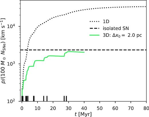
Comparison of the momentum evolution of 1D and 3D simulations of the same cluster (simulations 1D_06_HD and 3D_20_HD, respectively). The ‘isolated SN’ value is estimated using the first SN of the 3D_20_HD simulation, although it does not vary substantially between any of our 3D simulations.
This cannot be explained just by the fact that the 3D simulation has a lower initial resolution. In our previous work we tested the resolution dependence in our 1D simulations, and found that even with an initial spatial resolution of 5 pc, we still measured a terminal momentum yield roughly 10 times higher than what we find in our 3D simulation here as long as we ran our code in pseudo-Lagrangian rather than Eulerian mode (fig. 14 Gentry et al. 2017). So the problem is not convergence in our 1D simulation, but we have not yet shown whether our 3D results are converged.
To test for convergence in our 3D simulations, we compare our simulations which differ only in resolution (3D_07_HD, 3D_10_HD, 3D_13_HD, 3D_20_HD, and 3D_40_HD); in Fig. 2, we show the momentum evolution of each simulation. From that figure, we conclude that our 3D simulations do not appear converged, unlike our 1D simulations. The terminal momentum yield is increasing monotonically as we increase the resolution, so our 3D results are converging in the direction of our 1D results, but even at the highest resolution we can afford the momentum yield remains well below the 1D case. Thus we do not know if the 3D results would converge to the same value as the 1D case, even with infinite resolution.

Resolution study of our 3D HD simulations.
We further illustrate the non-convergence in Fig. 3, which shows the momentum of the shell at 6.46 Myr, the latest time we are able to reach at all resolutions. As the figure shows, with the exception of the lowest resolution run there is a clear trend of increasing momentum at higher resolution; we discuss possible explanations for the anomalous behaviour of the lowest resolution run in Appendix B. A simple power-law fit to the points at resolutions of Δx0 = 2 pc or better suggests that the momentum is increasing with resolution as |$p \propto \Delta x_0^{-0.16}$|. If we naively extrapolate this trend to the peak initial resolution of 0.03 pc achieved in our 1D simulations, the predicted momentum would be a factor of ∼2 larger than the highest resolution run shown, though this may well be an underestimate since Fig. 3 shows that the momentum appears to increase with resolution somewhat faster than predicted by a simple power-law fit. In any event, it is clear that, even at a resolution of 0.7 pc, our results are not converged.
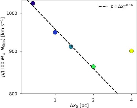
Resolution study of our 3D HD simulations at the last time achieved by all simulations. Colours are consistent with the resolution study figures above. The black dashed line shows the best power-law fit to all 3D HD simulations except the worst resolution simulation (3D_40_HD). Both axes are plotted using log scales.
To gain additional insight into the resolution-dependence of our results, and the differences between the 1D and 3D runs, we show a density slice through the centre of simulation 3D_20_HD at t = 7.53 Myr shown in Fig. 4. Clearly in 3D, the interface between the hot bubble interior and the cold shell is not spherically symmetric. These anisotropies are the result of physical instabilities (such as the Vishniac instabilities and the Rayleigh–Taylor instability) amplifying numerical inhomogeneities in the background ISM (Vishniac 1983, 1994; Mac Low & McCray 1988; Mac Low & Norman 1993; Krause et al. 2013; Fierlinger et al. 2016; Yadav et al. 2017). To see how this might affect the terminal momentum, we turn to density–temperature phase diagrams which are shown in Fig. 5. These phase diagrams correspond to a time soon after the sixth SN, with a delay long enough to allow the injected energy to spread throughout the bubble but sufficiently short to avoid significant energy losses due to cooling in any simulation. All 3D simulations have about 1.1 × 1051 erg more total energy than the start of the simulations, but 1D_06_HD retains more energy from previous SNe, and contains about 2.7 × 1051 erg of total energy relative to the simulation start. When we look at the mass-weighted phase diagram for our highest resolution completed simulation (3D_10_HD), we see that the mass is dominated by a cold dense shell, with a minority of mass in less-dense warm and hot phases (>103 K).8 Even when we vary the resolution, we only find negligible changes in the fraction of mass in the cold phase; the cold phase (T < 103 K) contributes 99.2 per cent of the affected mass in every completed simulation of our resolution study (3D_10_HD, 3D_20_HD, and 3D_40_HD). What does change is the density and temperature distribution of the warm/hot gas (T > 103 K). As we increase the resolution, the warm/hot gas shifts to lower and lower densities. This effect is very apparent for gas near the peak of the cooling curve (specifically 3 × 10⁴ K <T < 3 × 10⁵ K), which has a mass-weighted median density of ∼10−1mH cm−3 in our lowest resolution run, and ∼10−2mH cm−3 in our highest resolution completed run.

Reference density slice of the median resolution completed 3D simulation (3D_20_HD) at t = 7.53 Myr, approximately 0.03 Myr after the sixth SN.
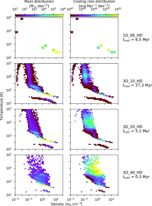
Phase diagrams for our completed HD simulations at t = 7.53 Myr, about 0.03 Myr after the sixth SN, when all simulations still retain almost all of the energy from the most recent SN. The left column shows the distribution of mass within temperature-density space, and the right column shows the cooling rate distribution within the space. The rows show the non-magnetized simulations with initial resolution worsening from top to bottom. To the right of each row, we give the cooling time of each simulation, |$t_\mathrm{cool} \equiv E_\mathrm{int} / \dot{E}_\mathrm{cool}$|, for reference.
This has a significant impact on the overall cooling times of the simulations. The right column of Fig. 5 shows that while the cold, dense phase dominates the mass, the minority of mass in the warm/hot phases dominates the cooling rate. This is important because resolution primarily affects these warm/hot phases, and it affects those phases by shifting them to higher densities at lower resolution, causing each particle to become more efficient at cooling. This results in significantly shorter cooling times: from 27 Myr at the best resolution to 0.3 Myr at the worst resolution, nearly two orders of magnitude difference. This increase primarily occurs in the warm/hot phases; at all resolutions gas warmer than 103 K constitutes slightly less than 1 per cent of the total mass, but this mass is responsible for 81 per cent of the cooling at our highest resolution completed run, and |$\gt 99{{\ \rm per\ cent}}$| of the cooling at our lowest resolution.
When we look at the phase diagrams for our 1D simulation, we see significant differences in the distributions of mass and cooling rate, leading to the very different behaviour of the 1D simulation. In particular, the 1D simulation completely lacks material at intermediate densities (∼10−2−100mH cm−3) due to how well the 1D simulation retains the contact discontinuity. The diffuse bubble-dense shell transition occurs within only a few cells, and the entire dense shell is resolved by just 5–10 cells. In our 3D simulations, these intermediate densities contribute a negligible amount of mass, but are responsible for much of the cooling. Without this intermediate phase material, almost all of the cooling in the 1D simulation occurs in the dense shell. We defer further discussion about the physical nature of the intermediate-temperature gas, and to what extent its properties are determined by physics versus numerics in the various simulations, in Section 4.
3.2 Magnetic fields
In Section 3.1, we showed that our numerical methods and resolution are not sufficient to achieve converged values of final radial momentum and other key parameters due to physical instabilities that develop within the superbubble shell. As described in Section 1, we expect that magnetic fields might affect the growth of physical instabilities, so we also run an MHD simulation as described in Section 2.2 to test the impact of magnetic fields on the final momentum. While the more standard method of extracting momentum, pmax, quoted in Table 2 appears to show that the inclusion of magnetic fields significantly decreases the final momentum, in this subsection we show that that method for estimating the asymptotic momentum (finding the maximum momentum following the last SN) is an oversimplification for simulations with magnetic fields. When we better isolate the momentum added by SNe, we find that adding magnetic fields can actually increase the momentum yield at fixed resolution. Indeed, our Δx0 = 2.0 pc MHD run produces a larger momentum injection than our Δx0 = 1.0 pc HD run.
First, to illustrate why the interpretation of the MHD simulation is more complex, in Fig. 6 we compare its momentum evolution to those of the non-magnetized simulations. The MHD simulation initially shows an increased momentum yield relative to the corresponding simulation without magnetic fields at the same resolution (3D_20_MHD), but then the momentum decreases due to magnetic tension forces. The reason for this is obvious if we examine a density slice at an earlier time, 9 as shown in Fig. 7: the expanding shell bends magnetic field lines outward, and the field lines exert a corresponding magnetic tension that reduces the radial momentum of the expanding shell. This effect is so strong that the momentum peaks after just seven SNe; the remaining four SNe clearly add momentum but not enough to overcome the steady decline.
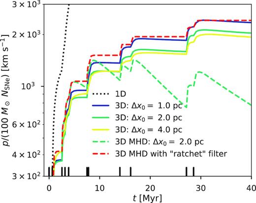
Same as Fig. 2, except now including the momentum evolution of our MHD simulation (3D_20_MHD; blue dashed curve), as well its ‘ratchet’-filtered momentum evolution, pratchet (red dashed curve), and excluding our incomplete HD runs (3D_07_HD and 3D_13_HD).

Same as Fig. 4, except now for simulation 3D_20_MHD with approximate magnetic field lines overplotted, and at an earlier time (t = 2.56 Myr; approximately 0.02 Myr after the third SN).
Due to this effect, the quantity pmax (the maximum momentum after the last SN) that we have used to characterize the hydrodynamic simulations is somewhat misleading, since our goal is to study the momentum injected by SNe, not the combined effects of SNe and magnetic confinement. To avoid this, we define an alternative quantity pratchet. To compute this quantity we sum any positive changes in radial momentum between snapshots, while ignoring any negative changes. We plot pratchet in Fig. 6, and report the final value in Table 2. As expected, for the non-magnetic runs pratchet and pmax are essentially the same, and thus examining pratchet allows us to make an apples-to-apples comparison between the magnetic and non-magnetic results.
This comparison is revealing, in that it shows that our simulation with magnetic fields (3D_20_MHD) injects about 10 per cent more momentum than the analogous simulations without magnetic fields (3D_20_HD). The full explanation for this difference will likely be complicated – for example, the bubble morphology and phase structure are significantly altered at late times relative to the non-magnetized runs – but we can see if our results are at least consistent with the hypothesis that magnetic fields could inhibit the growth of instabilities, leading to less phase mixing and cooling. To test this hypothesis, we compare phase diagrams for the resolution-matched magnetized and non-magnetized runs in Fig. 8, shown at the same time (t = 2.56 Myr) as Fig. 7. There we see that magnetic fields have an effect similar to that of increasing resolution in Fig. 5: both suppress the growth of fluid instabilities, causing the material near the peak of the cooling curve to stay at lower densities where it cools less efficiently. For gas near the peak of the cooling curve (specifically 3 × 10⁴ K <T < 3 × 10⁵ K), the median density of the non-magnetized run is 1.7 × 10⁻¹mH cm−3, while in the magnetized run it is 1.4 × 10⁻¹mH cm−3 – a modest change, but a change in the predicted direction. As a result the overall cooling time is about two times longer in the MHD run. Thus by suppressing the growth of instabilities, the inclusion of magnetic fields results in a longer overall cooling time which should contribute to a higher yield of momentum.

4 ANALYSIS
In Section 3, we showed our broad results, which have three key features: (1) Our 1D Lagrangian simulation finishes with about 10 times more momentum than our 3D simulations, and is converged with respect to resolution. (2) Our 3D HD simulations show a general increase in momentum as resolution improves, but are not converged even at the highest resolutions we can reach [similar to the 1D Eulerian simulations of Gentry et al. (2017), which are not converged even at a resolution of 0.31 pc]. (3) Our MHD simulations show less momentum than the resolution-matched HD simulation when the momentum is estimated directly, but more momentum when our ‘ratchet’ filter is used.
The phase diagrams shown in Figs 5 and 8 reveal that the changes in momentum budget appear to be associated with changes in the total mass and mean density of gas at temperatures of ≈105 K, near the peak of the cooling curve, which dominates the cooling budget. In this section we seek to understand the physical origin of these differences, with the goal of understanding whether the converged 1D or non-converged 3D results are likely to be closer to reality.
4.1 What determines convergence or non-convergence?
As a first step in this analysis, we investigate why our 1D Lagrangian simulations are converged while our 3D simulations are not. A simplistic view of superbubble cooling is one where the diffuse bubble interior contains most of the thermal energy but is radiatively inefficient, while the cold dense shell is radiatively efficient but does not have significant amounts of thermal energy to radiate. The cooling rate is then set by how quickly energy can transfer from one phase to the other.
This expression assumes a supersonic shock, and that all of the energy that is converted from kinetic to internal energy is immediately radiated away. At each simulation snapshot, we can compute Rshock and Vshock10 and compute the expected cooling rate using equation (2). We can then compare that to the observed cooling rate, calculated by grackle for each snapshot.
We begin our predicted-versus-actual cooling rate comparisons with our 1D Lagrangian simulation (1D_06_HD) shown in the top panel of Fig. 9. In that figure we can see that even though our mechanical shock model is simple, it does a generally good job predicting the observed cooling rate. On the other hand, we can repeat this with a simulation that is identical to 1D_06_HD except it uses an Eulerian hydrodynamic solver, leading to the results shown in the middle panel of Fig. 9. This reveals a very different picture: there are many times when the observed cooling rate is over an order of magnitude greater than our mechanical shock model would predict. And when the observed rate is lower than predicted, it is because the shell has already transitioned from a non-linear shock to a linear sound wave, for which we know equation (2) should not hold. While the mechanical shock model can explain most of the behaviour behind the 1D Lagrangian simulation, in the 1D Eulerian simulation the chosen numerical methods lead to much higher cooling rates which must be powered by additional thermal energy being pumped into the shell. When we apply this same approach to one of our 3D Lagrangian simulations (specifically simulation 3D_20_HD, shown in the bottom panel of Fig. 9), we find a behaviour similar to the 1D Eulerian simulation and very different from the 1D Lagrangian simulation: the actual cooling rates often far exceed the rate predicted by our mechanical shock cooling model.
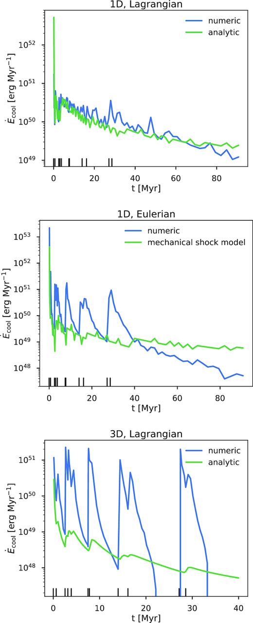
Comparison of the numeric cooling rate with the cooling rate predicted by our mechanical shock model, equation (2), for our 1D Lagrangian simulation (1D_06_HD; top), our 1D Eulerian simulation (1D_06_HD, but run with the code in Eulerian mode; middle), and our 3D HD simulation with 2 pc initial resolution (3D_20_HD; bottom).
This analysis makes it clear why the 1D Lagrangian simulations are converged: the radiative cooling rate has reached the minimum allowed by the physical situation of an adiabatic fluid doing work on a medium with a short radiative cooling time. Consequently, increasing the resolution cannot further reduce the rate of radiative loss; it is already as low as physically allowed. If we run the same problem in 1D Eulerian mode, or in 3D but at much lower resolution, the cooling rate is far in excess of the minimum. Cooling is powered not primarily by adiabatic compression of the cold gas followed by radiative loss, but by direct transfer of thermal energy between the hot and cold phases without doing any mechanical work. The rate of transfer is clearly resolution-dependent, which explains why the 1D Eulerian and 3D simulations are not converged.
4.2 Conduction and numerical mixing across the interface
Since the key difference between the converged 1D Lagrangian simulations and the unconverged 3D simulations is the relative importance of energy transfer by mechanical work versus other mechanisms, we next investigate the expected rate of non-mechanical energy transfer in reality, and how that compares to the rate in our simulations.
In our simulations, as opposed to reality, the width of the interface is set by numerical resolution. We illustrate this point in Fig. 10, which shows temperature and density slices from our highest resolution simulation (3D_07_HD) shortly after the second SN. We summarize the physical properties of the hot–cold interface, defined as material between 3 × 10⁴ K and 3 × 10⁵ K, roughly corresponding to the peak of the cooling curve, in Table 3; we include 3D_40_HD for completeness, but warn that, at this early time, its interface is poorly sampled by only 16 particles, and thus the results for it are not particularly meaningful. The main conclusion to make from Fig. 10 and Table 3 is that the physical width of the interface region is of order a particle smoothing length, so the width of the interface is determined by numerics rather than physics.

Density (top) and temperature (bottom) slices of the highest resolution 3D simulation (3D_07_HD) at t = 1.01 Myr, approximately 0.5 Myr after the second SN. The lighter cyan and darker red contours correspond to temperatures 3 × 10⁴ K and 3 × 10⁵ K, respectively, which are roughly the bounds of the peak of the cooling curve.
Interface properties at t = 1.01 Myr (0.5 Myr after the second SN). Here Npaticles and m are the number of particles and total mass in the interface (defined as the set of particles with temperatures in the range 3 × 10⁴−3 × 10⁵ K, near the peak of the cooling curve), rmedian is the median radius of interface particles, hmedian is the median scale length of interface particles, ΔrIQR is the interquartile range of interface particle radii.
| Name | Nparticles | m | rmedian | hmedian | ΔrIQR | ΔrIQR/hmedian |
|---|---|---|---|---|---|---|
| (M⊙) | (pc) | (pc) | (pc) | |||
| 3D_40_HD | 16 | 33.6 | 37.0 | 15.4 | 8.5 | 0.6 |
| 3D_20_HD | 159 | 41.8 | 39.1 | 9.8 | 8.3 | 0.8 |
| 3D_13_HD | 485 | 37.8 | 43.3 | 6.6 | 6.4 | 1.0 |
| 3D_10_HD | 1303 | 42.8 | 45.4 | 4.9 | 5.1 | 1.0 |
| 3D_07_HD | 4436 | 43.2 | 47.4 | 3.3 | 4.3 | 1.3 |
4.3 The role of 3D instabilities
Before accepting the conclusion that artificial conduction is the culprit for our non-convergence, however, we should examine an alternative hypothesis. The total conductive transport rate (equation 4) depends not just on the conductive flux, but on the area of the interface. Examining Fig. 10, it is clear that the area of the interface is affected by 3D instabilities that are not properly captured in the 1D simulations. Could the non-convergence in 3D be a result of the area not being converged, rather than the conductive flux not being converged? This hypothesis might at first seem plausible, because many instabilities (such as the Rayleigh–Taylor, Richtmyer–Meshkov, and Vishniac) initially grow fastest at the smallest scales (e.g. Taylor 1950; Richtmyer 1960; Vishniac 1983; Michaut et al. 2012). If the area of the interface is determined by the amount of time that it takes perturbations to grow from the resolution scale that might explain why our highest resolution simulation has the lowest cooling rate: because it had the smallest perturbations to start, and it has the smallest interface area later on, and thus the smallest rate of conduction.
However, we can ultimately rule out this hypothesis for two reasons. First, if the rate of mixing and radiative loss were set by processes developing from grid-scale perturbations, then changing the initial perturbation strength and scaling should have a noticeable impact on the cooling rate. However, as shown in Appendix A, our non-convergence is quite robust to the details of the grid-scale perturbations. The results are not any more converged when we impose perturbations whose power spectral density is independent of resolution over all resolved scales, and increasing the initial perturbation strength by a factor of >25 has negligible effects on the outcome. Second, once they are strongly non-linear, interface instabilities are typically dominated by larger rather than smaller modes. Examining Fig. 10, it is clear that even just after the second supernova we already have strongly non-linear perturbations in the shell, with each spike well resolved by many particles. If linear growth of instabilities from the grid scale were the source of our non-convergence, we would expect to see the greatest resolution dependence at early times, when the perturbations are smallest, and convergence between the runs at later time, when the instabilities reach non-linear saturation. Examining Fig. 2, however, shows exactly the opposite pattern: resolution matters more at later times than at earlier ones.
However, simply because we can rule out the hypothesis that the non-convergence of the 3D simulations is a result of our failure to capture the growth of 3D instabilities, it does not follow that the instabilities are not important. Fig. 10 clearly shows that the area of the interface in 3D is clearly larger than |$4 {\pi} R_{\rm shock}^2$|, and thus the rate of conduction across the interface should be higher than it is in our 1D simulations. Thus while our 3D simulations represent a lower limit on the terminal momentum, we must regard the 1D simulations as representing an upper limit, since the interface in 1D has the smallest possible area.
5 CONCLUSIONS
In this paper, we revisit the question of whether clustering of SNe leads to significant differences in the amount of momentum and kinetic energy that supernova remnants deliver to the ISM. This question is strongly debated in the literature, with published results offering a menu of answers that range from a relatively modest increase or decrease (Kim & Ostriker 2015; Walch & Naab 2015; Kim et al. 2017) to a substantial increase (Keller et al. 2014; Gentry et al. 2017). We investigate whether this discrepancy in results is due to numerical or physical effects, and to what extent it might depend on whether the flow is modelled as magnetized or non-magnetized.
Our results offer some encouragement and also some unhappy news regarding the prospects for treating supernova feedback in galactic and cosmological simulations. The encouraging aspect of our findings is that we have identified the likely cause of the discrepancy between the published results. We find that the key physical mechanism driving the differences between our runs, and almost certainly between other published results, is the rate of mixing across the contact discontinuity between the hot interior of a superbubble and the cool gas in the shell around it. Our 1D Lagrangian results (Gentry et al. 2017) maintain the contact discontinuity nearly perfectly, and give it the smallest possible area, and this explains why they produce large gains in terminal momentum per supernova due to clustering. However, these results likely represent an upper limit on the momentum gain, because they do not properly capture instabilities that increase the area of the contact discontinuity and thus encourage mixing across it.
In 3D, both physical instabilities and numerical mixing produce intermediate temperature gas that radiates rapidly and saps the energy of the superbubble, lowering the terminal momentum. Due to this mixing, we are unable to obtain a converged result for the terminal momentum; we find that the terminal momentum continues to increase with resolution even at the highest resolution that we complete (1 pc initial linear resolution, 0.03 M⊙ mass resolution). The cause of this effect is clear: as we increase the resolution, we find that the mean density and total mass of gas near the peak of the cooling curve continuously decreases (indicating a decrease in mixing), and this typically leads to a decrease in the amount of energy lost to radiation. Consequently, we are forced to conclude that even at our highest resolution in 3D, the mixing and energy transfer rate across the contact discontinuity is dominated by numerical mixing. As a result, our estimate of the momentum per supernova is only a lower limit.
Our tests with magnetic fields reinforce this conclusion. We find that magnetic fields suppress the growth rate of physical instabilities. This leads an magnetized simulation to inject more momentum per supernova than a non-magnetized simulation, but both still inject far less than the no-mixing case. This is consistent with the conclusion that physical mixing is present in our simulations but numerical mixing is the dominant source. In the real ISM, magnetic fields are doubtless present, so this effect should not be neglected, especially in simulations that are not dominated by numerical mixing.
Our findings cloud the prospects for obtaining a good first-principles estimate of the true supernova momentum yield in a homogeneous ISM. Our peak spatial resolution is higher than that achieved in previous 3D simulations, and we used Lagrangian methods rather than Eulerian methods. We note that our choice of Lagrangian rather than Eulerian methods was based on a 1D rather than 3D experiment, and that our results are likely affected by multiple definitions of resolution, such as the mass resolution of ejecta, and not just the peak spatial resolution. None the less, we are unable to reach convergence. We are forced to conclude that the true momentum yield from clustered SNe in a homogeneous ISM remains substantially uncertain. At this point we can only bound it between ≈2.4 × 10⁵ M⊙ km s−1 per SN (our non-converged 3D result) and ≈3.4 × 10⁶ M⊙ km s−1 per SN (our converged but 1D result). The 1D result certainly produces too much momentum, since 3D instabilities must enhance the conduction rate at least somewhat by increasing the area of the hot–cold interface. Similarly, our 3D results produce too little momentum, since our 3D results remain dominated by numerical conduction even at the highest attainable resolution; we do not know how close a converged 3D result would lie to the 1D, no-mixing limit.
We conclude by noting that we have not thus far investigated the effects of using a realistically turbulent, multiphase ISM. The presence of density inhomogeneities could well lead to higher rates of mixing across the contact discontinuity, and thus a reduction in the supernova momentum yield. However, we urge caution in interpreting the results of any investigations of these phenomena, since we have shown that even state-of-the-art simulation methods operating at the highest affordable resolutions cannot reach convergence in what should be substantially simpler problems. It is conceivable that the more complex density field of a realistic ISM might make it easier to reach convergence, but such a hope would need to be demonstrated rigorously using convergence studies in multiple numerical methods.
ACKNOWLEDGEMENTS
We thank Peter Mitchell for useful feedback on the role of shock cooling within our 1D simulations. This work was supported by the National Science Foundation (NSF) through grants AST-1405962 (ESG and MRK), AST-1229745 (PM), and DGE-1339067 (ESG), by the Australian Research Council through grant ARC DP160100695 (MRK), and by NASA through grant NNX12AF87G (PM). This research was undertaken with assistance of resources and services from the National Computational Infrastructure (NCI), which is supported by the Australian Government. MRK thanks the Simons Foundation, which contributed to this work through its support for the Simons Symposium ‘Galactic Superwinds: Beyond Phenomenology’. PM thanks the Préfecture of the Ile-de-France Region for the award of a Blaise Pascal International Research Chair, managed by the Fondation de l’Ecole Normale Supérieure. AL acknowledges support from the European Research Council (Project No. 614199 ‘BLACK’; Project No. 740120 ‘INTERSTELLAR’).
Footnotes
Throughout this paper we will quote temperatures calculated by grackle which accounts for temperature dependence in the mean molecular weight, μ (Smith et al. 2017).
This cluster can be found in the tables produced by Gentry et al. (2017) using the id 25451948-485f-46fe-b87b-f4329d03b203.
Our modifications of gizmo and our analysis routines can be found at: github.com/egentry/gizmo-clustered-SNe.
While this approach leads to a well-sampled injection kernel at our higher resolutions, the kernel is only sampled by about five new particles for each SN in our lowest resolution run, 3D_40_HD. This undersampling is not ideal and might slightly alter the bubble’s evolution, but the stochasticity this introduces does not appear to affect our conclusions.
The only exceptions are simulations 3D_07_HD and 3D_13_HD, which cannot be run to completion because they have smaller box sizes in order to minimize computational expense. These simulations are run until the shock approximately reaches the edge of the box. They are not meant to provide final values, but rather to enable us to investigate convergence of the results up to the times when these runs end.
The exact velocity threshold is somewhat arbitrary, leading to roughly 10 per cent uncertainty in the affected mass depending on the chosen threshold.
We estimate the isolated SN momentum yield, 2.4 × 10⁵ M⊙ km s−1, using the first SN of our 3D_20_HD simulation, although all of our 3D simulations would give the same value within a few per cent. This is approximately consistent with previous single SN simulations (e.g. Kim & Ostriker 2015; Martizzi et al. 2015).
We also see a negligible amount of mass at unusually low temperatures, <100 K. These particles are SN ejecta, which have very high metallicities that have been frozen-in due to the Lagrangian nature of the code.
We chose to look at an earlier snapshot, when the magnetization has only perturbed the bubble structure, rather than the later time shown in Fig. 4, when the magnetization would have caused a strong, non-linear change in the structure which could not be treated as a perturbation. In both cases the magnetic tension is present, but the earlier time makes it more straightforward to compare to the non-magnetized runs.
For our 3D simulations, we estimate Rshock as the mean radius of the overdense particles and Vshock as the mean radial velocity of the overdense particles. For our 1D simulations, we determine Rshock as the outermost overdense cell (see Gentry et al. 2017), and determine Vshock by taking the difference of Rshock between snapshots.
The variant of 3D_10_HD with the additional perturbation has only been run for about 15 Myr due to its computational cost, but we do not expect our conclusions would change if it were run to completion.
REFERENCES
APPENDIX A: SENSITIVITY TO INITIAL PERTURBATIONS
In the fiducial 3D simulations presented in the main text, we set up the initial gizmo particle positions by placing them in a uniform grid and then randomly perturbing each particle position using a Gaussian kernel with a dispersion of 10−3 times the initial spatial resolution. This results in an uncorrelated artificial density perturbation with a standard deviation of about 2 × 10⁻⁴ times the mean density as inferred by gizmo’s density solver, regardless of resolution.
In order to understand the effect of this perturbation, and how our results depend on its magnitude and whether that magnitude scales with resolution, we rerun a subset of our simulations with an additional perturbation. In addition to the artificial coordinate-based perturbation, we apply a ‘physical-like’ perturbation field directly to the particle masses and densities. To realize this, we generate a white (uncorrelated) Gaussian perturbation field with a magnitude of 5 per cent of the mean density sampled on the grid of our highest resolution completed simulation (3D_10_HD). For our lower resolution runs, we average the perturbation over appropriately larger apertures, matching what should happen if this were a physical perturbation. This averaging results in a decreasing perturbation magnitude at worsening resolution, but the magnitude is always at least a factor of 25 larger than the standard coordinate-based perturbation, and the power spectral density of the perturbation is the same at all resolved scales in all simulations. This resolution-dependence is a key difference from the artificial perturbation in our primary runs which has a magnitude that does not change with resolution. This process also introduces minor spatial correlations, as some higher resolution particles are equidistant between lower resolution particles, and their perturbation must be shared between multiple lower resolution particles.
In Fig. A1, we show the results of rerunning our three completed 3D HD simulations (3D_10_HD, 3D_20_HD, and 3D_40_HD) with these alternative initial conditions.11 We find that the details of the initial perturbation has very little effect compared to changing the resolution; increasing the perturbation magnitude by a factor of more than 25 has a smaller effect than increasing the spatial resolution by a factor of 2.

Comparison of the momentum evolution of our completed 3D simulations (3D_10_HD, 3D_20_HD, 3D_40_HD), and similar simulations with an additional, stronger perturbation with magnitudes that correctly scale with resolution.
APPENDIX B: SIMULATION 3D_40_HD AS AN OUTLIER AT EARLY TIMES
In the resolution study (e.g. Fig. 2) we see that the momenta of our simulations are well-ordered with respect to resolution at late times but that between the second and third SNe our lowest resolution simulation (3D_40_HD) has more momentum than our highest resolution simulation (3D_07_HD). We conjecture that this anomalous behaviour of 3D_40_HD is related to our SN injection method. As noted in Section 3.1, a typical SN is added using only ∼5 new particles in 3D_40_HD, leading to an undersampled injection kernel. While it is not clear precisely why undersampling would lead to a systematic increase in momentum, it is strongly suggestive that our simulations start behaving differently right as we hit the resolution limit of one of our methods.
Fortunately, this does not appear to affect our late-time results or our major conclusions. At early times, we recommend treating 3D_40_HD as an outlier, in which case the momentum will be monotonic with respect to resolution at effectively all times.
