


ABSTRACT
Various surveys focusing on the magnetic properties of intermediate-mass main-sequence (MS) stars have been previously carried out. One particularly puzzling outcome of these surveys is the identification of a dichotomy between the strong (|${\gtrsim }100\, {\rm G}$|), organized fields hosted by magnetic chemically peculiar (mCP) stars and the ultraweak (|${\lesssim }1\, {\rm G}$|) fields associated with a small number of non-mCP MS stars. Despite attempts to detect intermediate strength fields (i.e. those with strengths ≳10 and |${\lesssim }100\, {\rm G}$|), remarkably few examples have been found. Whether this so-called magnetic desert, separating the stars hosting ultraweak fields from the mCP stars truly exists has not been definitively answered. In 2007, a volume-limited spectropolarimetric survey of mCP stars using the MuSiCoS spectropolarimeter was initiated to test the existence of the magnetic desert by attempting to reduce the biases inherent in previous surveys. Since then, we have obtained a large number of ESPaDOnS and NARVAL Stokes V measurements allowing this survey to be completed. Here, we present the results of our homogeneous analysis of the rotational periods (inferred from photometric and magnetic variabilities) and magnetic properties (dipole field strengths and obliquity angles) of the 52 confirmed mCP stars located within a heliocentric distance of |$100\, {\rm pc}$|. No mCP stars exhibiting field strengths |${\lesssim }300\, {\rm G}$| are found within the sample, which is consistent with the notion that the magnetic desert is a real property and not the result of an observational bias. Additionally, we find evidence of magnetic field decay, which confirms the results of previous studies.
1 INTRODUCTION
The generation and broader characteristics of magnetic fields of cool stars are reasonably well understood within the framework of stellar dynamo theory (e.g. Charbonneau 2010). In contrast, the origin of the magnetic fields of main-sequence (MS) stars more massive than about |$1.5\, M_\odot$| remains a profound mystery. Over the past several decades, many clues related to this problem have been reported.
It is now reasonably well established that all magnetic, chemically peculiar stars [i.e. Ap/Bp stars, hereinafter referred to as magnetic chemically peculiar (mCP) stars] host organized magnetic fields with strengths as large as |$30\, {\rm kG}$| (e.g. Landstreet 1982; Shorlin et al. 2002). In general, the large-scale structures of these fields are relatively simple (e.g. Babcock 1956; Kochukhov et al. 2015), although a few obvious examples of more complex fields have been discovered (e.g. Kochukhov et al. 2011; Silvester et al. 2017). Furthermore, both young and evolved MS mCP stars are known to exist (e.g. Wade 1997; Kochukhov & Bagnulo 2006), which suggests that these fields are stable over long time periods. Surface magnetic fields have been detected on some Herbig Ae/Be stars (e.g. Wade et al. 2007; Alecian et al. 2013), which are likely the progenitors of the MS mCP stars. All of these findings are consistent with the notion that the fields hosted by mCP stars are fossil remnants left over from an earlier stage in the star’s evolution (the fossil field theory, Cowling 1945; Moss 1984; Landstreet 1987).
One property of stellar magnetism of upper MS stars that is not currently well explained by the fossil field theory is the fact that only ∼10 per cent of all MS A- and B-type stars (e.g. Wolff 1968; Smith 1971) host strong, organized surface magnetic fields. Shorlin et al. (2002), Bagnulo et al. (2006), and Aurière et al. (2010) obtained a large number of magnetic measurements of non-mCP MS stars of spectral types A and B with median uncertainties of 20, 95, and |$2\, {\rm G}$|, respectively, however, no magnetic detections were reported. Makaganiuk et al. (2010) carried out a similar survey of HgMn stars – obtaining typical longitudinal field uncertainties |${\sim }10\, {\rm G}$| and as low as |$0.8\, {\rm G}$| – but did not report any detections of circularly polarized Zeeman signatures. Recently, fields with strengths |${\lesssim }1\, {\rm G}$| (so-called ultraweak, or Vega-type, fields) were detected on a small number of non-mCP stars (e.g. Lignières et al. 2009; Petit et al. 2011; Blazère, Neiner & Petit 2016). Based on these findings, Petit et al. (2011) speculate that a much higher fraction of MS A-type stars (i.e. ≫10 per cent) may host ultraweak surface fields. Regardless, the dichotomy between the strongly magnetic and the non-magnetic (or very weakly magnetic) MS A-type stars is unlikely to be entirely explained by the sensitivity of the current generation of spectropolarimeters. In the case of Vega, it is reported that its ultraweak field exhibits a highly complex field structure (Petit et al. 2010) that is atypical of the strongly magnetic mCP stars. It is therefore plausible that the ultraweak fields are a distinct phenomenon, which may have an origin that differs from that of the strong, organized fields hosted by mCP stars (Braithwaite & Cantiello 2013).
Aurière et al. (2007) explored the weak field regime of mCP stars by obtaining high-precision longitudinal field measurements of 28 such objects with reportedly weak or otherwise poorly constrained field strengths. All of the observed mCP stars were detected in their spectropolarimetric observations, and were inferred to exhibit dipolar field strengths of |$B_{\rm d}\gtrsim 100\, {\rm G}$| with the two weakest fields found to have |$B_{\rm d}=100_{-100}^{+392}$| and |$229_{-76}^{+248}\, {\rm G}$|. Aurière et al. (2007) hypothesized that there exists a critical field strength (|$B_{\rm c}\approx 300\, {\rm G}$|), which corresponds to the minimum field strength that an mCP star must host in order to be invulnerable to a magnetohydrodynamic pinch instability (Tayler 1973; Spruit 2002). In this scenario, every intermediate-mass MS star may be initially ‘assigned’ a field strength (perhaps based on external factors, e.g. the local field properties at its location of formation, the presence of a companion, etc.) drawn from a probability distribution that increases towards lower field strengths; only those fields exceeding Bc are able to be maintained, which results naturally in the so-called magnetic desert (i.e. the dichotomy between the ultraweak fields detected on a small number of non-mCP stars and the strong fields hosted by mCP stars, Lignières et al. 2014).
While the detection of ultraweak fields may not directly contradict the existence of a critical lower field strength limit, two stars have been found reportedly hosting fields with intermediate strengths (i.e. |$10\lesssim B_{\rm d}\lesssim 100\, {\rm G}$|, which is lower than the typical |$B_{\rm c}\sim 300\, {\rm G}$| proposed by Aurière et al. 2007). The massive early B-type star β CMa reportedly hosts a field with |$B_{\rm d}\lt 230\, {\rm G}$| (Fossati et al. 2015), while the primary component of the spectroscopic binary HD 5550 is reportedly an Ap star hosting a field having |$B_{\rm d}\lt 85\, {\rm G}$| (Alecian et al. 2016). We discuss these two examples in Section 7; however, we note that the fact that nearly all mCP stars are found hosting fields |${\gtrsim }100\, {\rm G}$| despite the current detection limits that have been achieved remains conspicuous.
A potential problem with many of the reported empirical properties of mCP stars – including the existence of the magnetic desert – is the fact that they are generally inferred from intrinsically biased surveys: they are either biased towards brighter objects (magnitude-limited surveys) or those hosting stronger, more easily detectable fields (field-strength limited surveys). In 2007, a volume-limited survey of mCP stars located within a heliocentric distance of |$100\, {\rm pc}$| was initiated by Power (2007) in order to reduce these observational biases. This work yielded the magnetic properties of a large number of mCP stars in the sample using measurements obtained with the now-decommissioned MuSiCoS spectropolarimeter at the Pic du Midi Observatory. However, at the completion of that investigation, nearly half of the sample remained either unobserved or had relatively poor constraints on their field strengths and geometries. We have recently completed this survey using measurements obtained by ESPaDOnS and NARVAL.
In Paper I, we described in detail the sample of mCP and non-mCP stars included in the volume-limited sample. This sample was compiled using Hipparcos parallaxes (ESA 1997) to identify all MS stars with masses |$\ge 1.4\, M_\odot$| (i.e. all early-F, A-, and B-type MS stars) located within the adopted distance limit of |$100\, {\rm pc}$|. We then cross-referenced this list with the Catalogue of Ap, HgMn, and Am stars (Renson, Gerbaldi & Catalano 1991; Renson & Manfroid 2009) as well as the Spectral Classifications compiled by Skiff (2014) in order to identify confirmed and candidate mCP stars. Ultimately, 52 confirmed mCP stars were identified based on published, archived, and newly obtained photometric, spectroscopic, and spectropolarimetric (i.e. Stokes V) measurements. We derived fundamental parameters (effective temperatures, luminosities, masses, ages, etc.) of all of the intermediate-mass MS stars in the sample. Average surface chemical abundances of the mCP stars were also derived. The analysis presented in Paper I serves as a starting point for the magnetic analysis presented here. The results included in this second paper (i.e. Paper II) are organized as follows.
In Section 2, we discuss the newly obtained or previously unpublished MuSiCoS, ESPaDOnS, and NARVAL Stokes V observations. In Section 3, we present our analysis of these measurements and how they are used to derive longitudinal magnetic field measurements; the measurements are then used to help identify each star’s rotational period, as discussed in Section 4. In Section 5, we derive the magnetic field strengths and geometries and in Section 6, we search for evolutionary changes of the field strengths. Finally, in Section 7, we discuss the results while presenting our conclusions drawn from the survey.
2 NEW OBSERVATIONS
2.1 MuSiCoS spectropolarimetry
The MuSiCoS échelle spectropolarimeter was installed on the |$2\, {\rm m}$| Télescope Bernard Lyot (TBL) at the Pic du Midi Observatory in 1996 where it was operational until its decommissioning in 2006. It had a resolving power |${\sim }35\, 000$| and was capable of obtaining circularly polarized (Stokes V) spectra from 3900 to |$8700\, {\rm \mathring{\rm A} }$| (Donati et al. 1999). For this study, we used a total of 151 Stokes V observations of 23 stars that were obtained from 1998 February 12 to 2006 June 8. These observations were reduced using the esprit software package (Donati et al. 1997) .
We note that the raw MuSiCoS spectra used in this study are unavailable and we have relied on normalized and reduced spectra from a private archive. All of the available spectra span a wavelength range of 4500–|$6600\, {\rm \mathring{\rm A} }$| rather than the full range presumably associated with the raw spectra. Furthermore, an automatic normalization routine built into the esprit reduction package had been applied to the spectra.
2.2 ESPaDOnS and NARVAL spectropolarimetry
The ESPaDOnS and NARVAL échelle spectropolarimeters are twin instruments installed at the Canada–France–Hawaii Telescope, and TBL, respectively. They have a resolving power |${\sim }65\, 000$| and are optimized for a wavelength range of approximately 3600–|$10\, 000\, {\rm \mathring{\rm A} }$|.
We obtained 95 Stokes V observations of 37 stars from 2015 August 02 to 2016 August 10 using ESPaDOnS. Twenty-three Stokes V observations of three stars were obtained using NARVAL from 2016 August 20 to 2017 February 20. All of the observations obtained using ESPaDOnS and NARVAL were reduced with the libre-esprit software package, which is an updated version of the esprit reduction package that was applied to the MuSiCoS data (Donati et al. 1997).
3 MAGNETIC MEASUREMENTS
Organized magnetic fields that are present in the photospheres of mCP stars may be detected by identifying Zeeman signatures in Stokes V spectropolarimetric observations. While these signatures are typically weak in individual spectral lines, the signal-to-noise ratios (SNRs) can be significantly increased by calculating least-squares deconvolution (LSD) profiles (Donati et al. 1997; Kochukhov, Makaganiuk & Piskunov 2010) . This cross-correlation technique involves essentially averaging a large number of spectral lines (typically ≳100) having similarly shaped profiles. It has been widely used in the study of mCP star magnetism (e.g. Wade et al. 2000; Shorlin et al. 2002).
3.1 Confirmed mCP Stars
We generated LSD profiles for all of the available Stokes V observations. This was carried out by first generating line lists containing wavelengths, depths, and Landé factors, from the Vienna Atomic Line Database (VALD, Ryabchikova et al. 2015). Custom lists specific to each star in the sample were obtained using Extract Stellar requests specifying the effective temperatures (Teff), surface gravities (log g), and chemical abundances derived in Paper I (solar abundances were adopted for those elements without estimated abundances); a microturbulence value (vmic) of |$0\, {\rm km\, s^{-1}}$| was used along with a detection threshold of 0.05 and a wavelength range of 4000–|$7000\, {\rm \mathring{\rm A} }$|. Line masks were subsequently generated from each of the line lists and compared with the observed spectra: any lines in the line mask that were found to overlap with either telluric lines or broad Balmer lines were removed. The Stokes V, Stokes I, and diagnostic null [i.e. the flux obtained by combining the subexposures such that the net polarization of the source is cancelled, equation (3) of Donati et al. 1997 measurements associated with each spectropolarimetric observation were normalized by fitting a multiorder polynomial to the continuum flux of each spectral order. An example of an LSD profile calculated using one of the observed spectra and its associated line mask is shown in Fig. 1. Additional examples are shown in the electronic version of this paper.
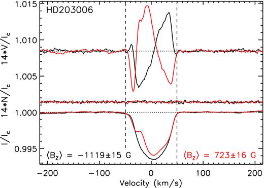
Two examples of the Stokes V (top), diagnostic null (middle), and Stokes I (bottom) LSD profiles derived from the spectropolarimetric observations obtained using ESPaDOnS. The vertical dashed lines indicate the adopted integration limits used to derive the displayed 〈Bz〉 values. Note that the Stokes V and diagnostic null profiles have been scaled by a factor of 14. Additional examples are included in the electronic version of this paper.
The Stokes I/Ic and V/Ic LSD profiles were used to measure the disc-averaged longitudinal magnetic field (〈Bz〉) as given by equation (1) of Wade et al. (2000). We used mean wavelengths (λavg) and mean Landé factors (zavg) calculated from the customized line masks associated with each star. Prior to each 〈Bz〉 measurement, the Stokes I/Ic and V/Ic LSD profiles were renormalized by fitting a first-order polynomial (i.e. a linear function) to the regions where I/Ic ∼ 1 and V/Ic ∼ 0 (typically at |$v\approx \pm 100\, {\rm km\, s^{-1}}$|). Any radial velocity shift that was apparent in the Stokes I/Ic LSD profile, as inferred from the calculation of the profile’s ‘centre of gravity’ (i.e. the integral of vI/Ic over that of I/Ic), was removed. The v integration limits were chosen to encompass the absorption profile as determined by eye. The derived values of 〈Bz〉 associated with the confirmed mCP stars are listed in Table 1.
Observations of confirmed mCP stars – those stars for which at least one definite detection was obtained based on the criterion proposed by Donati et al. (1997). Columns 1–5 contain the HD number, instrument used to obtain the observation (ESP = ESPaDOnS, MUS = MuSiCoS, and NAR = NARVAL), HJD, rotational phase, and the derived 〈Bz〉 value and its associated uncertainty. The full table will appear only in the electronic version of the paper.
| HD | Inst. | HJD | Phase | 〈Bz〉 | HD | Inst. | HJD | Phase | 〈Bz〉 |
|---|---|---|---|---|---|---|---|---|---|
| (G) | (G) | ||||||||
| 15089 | MUS | 3040.343 | 0.259 | 223 ± 93 | ESP | 7443.892 | 0.434 | −81 ± 36 | |
| MUS | 3586.543 | 0.077 | 450 ± 23 | ESP | 7447.848 | 0.739 | 86 ± 26 | ||
| MUS | 3589.652 | 0.864 | 506 ± 18 | 72968 | MUS | 3748.583 | 0.774 | 346.4 ± 8.4 | |
| MUS | 3590.561 | 0.386 | −258 ± 20 | MUS | 3749.549 | 0.945 | 343.0 ± 7.3 | ||
| MUS | 3591.597 | 0.981 | 509 ± 19 | MUS | 3755.429 | 0.985 | 307 ± 16 | ||
| MUS | 3594.551 | 0.678 | −166 ± 24 | MUS | 3756.527 | 0.179 | 323.5 ± 7.0 | ||
| MUS | 3607.557 | 0.150 | 441 ± 32 | ESP | 7416.994 | 0.763 | 334.1 ± 5.2 | ||
| MUS | 3616.513 | 0.296 | 11 ± 24 | ESP | 7498.720 | 0.221 | 335.2 ± 3.8 | ||
| 15144 | MUS | 2253.385 | 0.716 | −568 ± 13 | ESP | 7500.781 | 0.586 | 266.8 ± 2.5 | |
| MUS | 2254.408 | 0.057 | −619 ± 12 | 74067 | ESP | 7330.146 | 0.046 | 1024 ± 11 | |
| MUS | 3410.324 | 0.620 | −567 ± 18 | ESP | 7331.099 | 0.352 | −147 ± 10 | ||
| MUS | 3613.503 | 0.392 | −551 ± 15 | ESP | 7348.156 | 0.828 | 748 ± 38 | ||
| MUS | 3615.559 | 0.078 | −612 ± 10 | ESP | 7415.993 | 0.605 | −303 ± 12 | ||
| MUS | 3617.570 | 0.749 | −586 ± 11 | ESP | 7440.875 | 0.592 | −370 ± 34 | ||
| 18296 | ESP | 7556.127 | 0.190 | 91 ± 19 | ESP | 7445.857 | 0.192 | 562 ± 26 | |
| ESP | 7561.124 | 0.923 | 169 ± 19 | ESP | 7446.838 | 0.506 | −480 ± 28 | ||
| ESP | 7610.142 | 0.918 | 195.7 ± 9.7 | 96616 | ESP | 7358.169 | 0.668 | −58 ± 15 | |
| 24712 | MUS | 857.333 | 0.180 | 765 ± 13 | ESP | 7441.990 | 0.172 | 213 ± 16 | |
| MUS | 1924.360 | 0.830 | 763 ± 12 | ESP | 7444.970 | 0.399 | −153 ± 22 | ||
| MUS | 3247.675 | 0.052 | 1033 ± 17 | ESP | 7447.937 | 0.620 | −101 ± 13 | ||
| 56022 | ESP | 7325.149 | 0.210 | 139 ± 32 | ESP | 7448.964 | 0.043 | 325 ± 14 | |
| ESP | 7438.845 | 0.941 | 195 ± 24 |
In addition to the previously unpublished 〈Bz〉 measurements listed in Table 1, we also derived 〈Bz〉 from archived ESPaDOnS and NARVAL Stokes V observations. In these cases, we applied the same analysis that was used with the new observations reported in this study. This ensured that both the new and archived observations yielded consistent 〈Bz〉 measurements such that any apparent variability cannot be attributed to the use of different line masks (i.e. all 〈Bz〉 values are obtained using the same measurement system). In total, we used 400 measurements of 42 confirmed mCP stars derived using the line masks generated in this study – corresponding to a median value of six observations per star. These 〈Bz〉 measurements exhibit a median uncertainty of |$\sigma _{\langle B_{\rm z}\rangle }=18\, {\rm G}$|. Published 〈Bz〉 measurements exist for the majority of the confirmed mCP stars. We compiled and included many of these measurements in our analysis when no corresponding archival Stokes V observations were found. For 10 out of the 52 confirmed mCP stars, only previously published measurements were available (i.e. no new or archived Stokes V observations were available). Note that these published data are not derived using the same measurement system as used for the 〈Bz〉 measurements that we derived from the Stokes V observations and analysed herein.
In summary, a total of 947 new, archived, and published 〈Bz〉 measurements of the confirmed mCP stars were used in this study, corresponding to a median number of observations per star of 17. The measurements exhibit a median |$\sigma _{\langle B_{\rm z}\rangle }$| of |$49\, {\rm G}$| and a median minimum |$\sigma _{\langle B_{\rm z}\rangle }$| per star of |$15\, {\rm G}$|. For four of the 52 stars, fewer than five observations are available. Two detections of HD 117025 are reported by Kochukhov & Bagnulo (2006) while, due to its relatively low declination of −45°, we were only able to obtain a single observation of HD 217522. For HD 29305, only four archived HARPSpol Stokes V observations are available while for HD 56022, we obtained four new Stokes V observations using ESPaDOnS .
3.2 Null results
As discussed in Paper I, during the initial phase of this study, we identified a number of stars within the Catalogue of Ap, HgMn, and Am stars (Renson & Manfroid 2009) reported as being potential mCP members. Additionally, several Am and HgMn stars were found to exhibit Δa, Δ(V1 − G), or ΔZ photometric indices consistent with those exhibited by mCP stars (e.g. Maitzen, Pressberger & Paunzen 1998; Bayer et al. 2000; Paunzen & Maitzen 2005). We obtained Stokes V observations for 19 of these stars using MuSiCoS, ESPaDOnS, and NARVAL in order to search for Zeeman signatures. The observations were analysed using the same LSD technique that was applied to the confirmed mCP stars; however, the line masks generated from the VALD line lists used a surface gravity of |$\log {g}=4.0\, {\rm (cgs)}$| and a solar metallicity (individual chemical abundances were not specified).
No Zeeman signatures were detected from the observations of the 19 stars. The minimum 〈Bz〉 uncertainties obtained for each star ranged from 1.9 to |$69\, {\rm G}$| with a median value of |$11.4\, {\rm G}$|. Kochukhov & Bagnulo (2006) report a measured |$\langle B_{\rm z}\rangle =-56\pm 68\, {\rm G}$| for one of the 19 stars, HD 202627; we obtained a single observation of this star, which yielded a lower uncertainty and no detection (|$\langle B_{\rm z}\rangle =14\pm 17\, {\rm G}$|). The observations are summarized in Table 2 where we list the measured longitudinal field values.
Spectropolarimetric observations of those stars for which no Zeeman signatures were detected. Columns 1 –6 contain the HD number, instrument used to obtain the observation (ESP = ESPaDOnS, MUS = MuSiCoS, andNAR = NARVAL), HJD, exposure time, number of consecutive observations, and the derived 〈Bz〉 value and its associated uncertainty.
| HD | Instrument | HJD | texp (s) | Number | 〈Bz〉 (G) | HD | Instrument | HJD | texp (s) | Number | 〈Bz〉 (G) |
|---|---|---|---|---|---|---|---|---|---|---|---|
| |$+2\, 450\, 000$| | |$+2\, 450\, 000$| | ||||||||||
| 358 | ESP | 7561.129 | 15 | 1 | 31 ± 19 | MUS | 3747.683 | 3200 | 1 | 180 ± 180 | |
| 4853 | ESP | 7239.132 | 200 | 1 | 24 ± 19 | MUS | 3750.683 | 3200 | 1 | 70 ± 180 | |
| 27411 | ESP | 7435.763 | 8 | 1 | 0 ± 11 | MUS | 3755.683 | 3200 | 1 | 210 ± 160 | |
| 27749 | ESP | 7435.766 | 5 | 1 | 5.4 ± 9.5 | MUS | 3756.626 | 3200 | 1 | 80 ± 140 | |
| 67523 | ESP | 7414.991 | 5 | 1 | 0.5 ± 1.9 | MUS | 3864.422 | 2400 | 1 | 50 ± 220 | |
| 78362 | MUS | 858.604 | 1200 | 1 | −0.2 ± 3.9 | MUS | 3874.440 | 2400 | 1 | −90 ± 180 | |
| MUS | 1202.554 | 1635 | 1 | −8 ± 25 | MUS | 3885.401 | 2400 | 1 | 120 ± 240 | ||
| ESP | 7412.001 | 5 | 1 | −6.3 ± 5.7 | MUS | 3892.366 | 2400 | 1 | −20 ± 190 | ||
| 90763 | ESP | 7325.137 | 8 | 1 | 34 ± 54 | ESP | 7236.789 | 330 | 2 | 39 ± 26 | |
| ESP | 7327.160 | 8 | 1 | 79 ± 47 | ESP | 7261.749 | 330 | 2 | −47 ± 28 | ||
| ESP | 7328.157 | 8 | 1 | −18 ± 50 | ESP | 7262.733 | 330 | 2 | 10 ± 25 | ||
| ESP | 7329.106 | 8 | 1 | 60 ± 53 | ESP | 7265.730 | 330 | 2 | 3 ± 43 | ||
| ESP | 7330.122 | 31 | 1 | 6 ± 27 | 120025 | ESP | 7414.075 | 123 | 1 | −4.6 ± 8.2 | |
| ESP | 7522.802 | 60 | 1 | 12 ± 23 | 125335 | ESP | 7408.155 | 200 | 1 | −4.0 ± 3.2 | |
| 102942 | ESP | 7412.006 | 37 | 1 | −8 ± 10 | 136729 | NAR | 7800.669 | 3188 | 1 | 15 ± 68 |
| ESP | 7497.913 | 37 | 1 | 0 ± 10 | 139478 | NAR | 7801.609 | 1176 | 1 | −2.9 ± 7.6 | |
| ESP | 7498.878 | 200 | 2 | −4.3 ± 3.2 | 149748 | ESP | 7409.126 | 225 | 1 | 20 ± 13 | |
| ESP | 7500.885 | 200 | 2 | −4.0 ± 3.2 | 156164 | ESP | 7560.979 | 40 | 1 | 190 ± 290 | |
| 105702 | ESP | 7409.107 | 6 | 1 | 22 ± 17 | 189849 | ESP | 7476.130 | 19 | 1 | 3.8 ± 3.6 |
| ESP | 7495.949 | 6 | 2 | 11 ± 16 | 202627 | ESP | 7261.984 | 217 | 2 | 14 ± 16 | |
| ESP | 7497.923 | 6 | 1 | −16 ± 11 | 206742 | ESP | 7262.001 | 50 | 1 | −9 ± 26 | |
| ESP | 7498.955 | 6 | 1 | 13 ± 13 | ESP | 7262.001 | 50 | 1 | 71 ± 63 | ||
| ESP | 7500.902 | 6 | 1 | −15 ± 11 | 221675 | ESP | 7554.124 | 100 | 1 | −3 ± 13 | |
| 115735 | MUS | 1600.662 | 2595 | 1 | −100 ± 190 |
Parameters associated with the 〈Bz〉 curves shown in Figs 2 and 3. Columns 1–3 list each star’s HD number, adopted or derived rotational period, and the adopted epoch, respectively. References for those rotational periods taken from the literature are listed in the table’s footer; Prot values without references were derived in this study. Columns 4, 5, and 7 list the mean, amplitudes, and reduced χ2 values associated with the first-order sinusoidal fits sinusoidal (i.e. C0 and C1 in equation (1) with C2 ≡ 0). Column 6 lists the r parameters [equation (2) of Preston 1967.
| HD | |$P_{\rm rot}\, (\text{d})$| | HJD0 − 2.4 × 10⁶ | |$B_0\, ({\rm G})$| | |$B_1\, ({\rm G})$| | r | |$\chi ^2_{\rm red}$| |
|---|---|---|---|---|---|---|
| (1) | (2) | (3) | (4) | (5) | (6) | (7) |
| 3980 | |$3.9516(3)^{\, a}$| | 40927.2031 | 120 ± 1810 | 1710 ± 4470 | −0.87 ± 0.44 | 1.5 |
| 11502 | 1.60984(1) | 43002.93904 | −130 ± 230 | 730 ± 350 | −0.69 ± 0.21 | 3.8 |
| 12446 | |$1.4907(12)^{\, b}$| | 43118.3498 | −40 ± 84 | 470 ± 130 | −0.84 ± 0.07 | 0.8 |
| 15089 | |$1.74050(3)^{\, c,d}$| | 53039.89185 | 109 ± 63 | 463 ± 90 | −0.62 ± 0.10 | 6.6 |
| 15144 | 2.99799(1) | 52254.23776 | −581.6 ± 7.2 | 33.8 ± 9.9 | 0.89 ± 0.05 | 0.2 |
| 18296 | 2.88416(15) | 42999.22302 | 10 ± 210 | 210 ± 340 | −0.94 ± 0.16 | 0.7 |
| 24712 | |$12.4580(15)^{\, e}$| | 47179.9838 | 560 ± 160 | 510 ± 250 | 0.04 ± 0.39 | 3.6 |
| 27309 | |$1.5688840(47)^{\, f}$| | 52247.1353483 | −716 ± 80 | 100 ± 120 | 0.75 ± 0.43 | 3.0 |
| 29305 | |$2.943176(3)^{\, g}$| | 56967.257773 | 29.9 ± 1.3 | 74.7 ± 1.3 | −0.43 ± 0.01 | <0.1 |
| 38823 | 8.676(30) | 51894.778 | −460 ± 430 | 2040 ± 640 | −0.63 ± 0.16 | 24.7 |
| 40312 | 3.61866(2) | 42762.85334 | 91 ± 44 | 307 ± 62 | −0.54 ± 0.12 | 9.9 |
| 49976 | |$2.97666(8)^{\, h}$| | 41401.97078 | −380 ± 610 | 1960 ± 830 | −0.68 ± 0.20 | 3.2 |
| 54118 | |$3.27535(10)^{\, i}$| | 42114.75746 | 30 ± 250 | 1500 ± 330 | −0.96 ± 0.01 | 1.5 |
| 56022 | |$0.91889(3)^{\, g}$| | 57324.95641 | 79 ± 39 | 142 ± 75 | −0.29 ± 0.37 | 1.1 |
| 62140 | 4.28677(3) | 50505.89765 | −5 ± 57 | 1577 ± 77 | −0.993 ± 0.001 | 13.7 |
| 65339 | |$8.02681(4)^{\, j}$| | 50494.99521 | −50 ± 540 | 4740 ± 840 | −0.978 ± 0.006 | 58.8 |
| 72968 | 5.6525(10) | 52251.9491 | 318 ± 40 | 54 ± 66 | 0.71 ± 0.49 | 6.1 |
| 74067 | 3.11511(226) | 57326.88599 | 301 ± 38 | 761 ± 46 | −0.43 ± 0.04 | 1.6 |
| 83368 | |$2.851976(3)^{\, k}$| | 45063.924739 | −10 ± 260 | 730 ± 410 | −0.97 ± 0.03 | 1.7 |
| 96616 | 2.42927(2) | 57356.54706 | 79 ± 18 | 263 ± 25 | −0.54 ± 0.06 | 0.8 |
| 103192 | |$2.35666(2)^{\, i}$| | 43736.07566 | −206 ± 68 | 38 ± 99 | 0.7 ± 1.2 | 0.3 |
| 108662 | 5.07735(24) | 42214.90968 | −360 ± 210 | 410 ± 300 | −0.06 ± 0.61 | 53.5 |
| 108945 | 2.05186(12) | 51613.95547 | −23 ± 77 | 250 ± 100 | −0.83 ± 0.11 | 1.2 |
| 109026 | |$2.84(22)^{\, l}$| | 56336.96 | 309 ± 19 | 170 ± 29 | 0.29 ± 0.13 | 0.7 |
| 112185 | |$5.0887(13)^{\, m,n}$| | 41794.5148 | 19 ± 36 | 80 ± 45 | −0.62 ± 0.31 | 1.9 |
| 112413 | 5.46913(8) | 50503.70120 | −104 ± 96 | 770 ± 120 | −0.76 ± 0.06 | 184.8 |
| 118022 | |$3.722084(2)^{\, h}$| | 50499.616970 | −533 ± 55 | 438 ± 68 | 0.10 ± 0.14 | 2.2 |
| 119213 | |$2.4499141(38)^{\, o}$| | 53406.2587031 | 380 ± 110 | 300 ± 120 | 0.11 ± 0.37 | 2.6 |
| 120198 | |$1.38576(80)^{\, p}$| | 42769.49376 | 150 ± 210 | 330 ± 260 | −0.36 ± 0.61 | 1.1 |
| 124224 | |$0.52070308(120)^{\, q,r}$| | 42850.85176720 | 120 ± 180 | 960 ± 240 | −0.78 ± 0.09 | 7.0 |
| 128898 | |$4.4790(1)^{\, s}$| | 42116.9439 | −320 ± 180 | 120 ± 260 | 0.4 ± 1.4 | 1.4 |
| 130559 | 1.90798(1) | 53407.61250 | −280 ± 25 | 208 ± 32 | 0.15 ± 0.13 | 2.0 |
| 137909 | |$18.4877(15)^{\, t}$| | 46201.8254 | 60 ± 150 | 710 ± 190 | −0.84 ± 0.07 | 104.9 |
| 137949 | 5195 | 38166 | 1620 ± 100 | 170 ± 170 | 0.81 ± 0.27 | 1.8 |
| 140160 | 1.59587(11) | 51607.01456 | −10 ± 150 | 320 ± 180 | −0.97 ± 0.03 | 1.4 |
| 140728 | 1.29559(2) | 53864.86021 | −27 ± 35 | 514 ± 42 | −0.90 ± 0.01 | 0.3 |
| 148112 | 3.04416(112) | 52094.28900 | −180 ± 23 | 33 ± 35 | 0.69 ± 0.46 | 1.2 |
| 148898 | 2.3205(2) | 52764.4371 | 238 ± 83 | 390 ± 110 | −0.25 ± 0.23 | <0.1 |
| 151199 | 1.83317(22) | 53366.50581 | −81 ± 65 | 198 ± 92 | −0.42 ± 0.33 | 0.8 |
| 152107 | |$3.857500(15)^{\, u}$| | 53600.975034 | 961 ± 49 | 357 ± 64 | 0.46 ± 0.13 | 9.8 |
| 170000 | |$1.71649(2)^{\, v}$| | 42632.30626 | 123 ± 60 | 370 ± 82 | −0.50 ± 0.14 | 4.5 |
| 187474 | |$2345(15)^{\, w}$| | 45534 | −50 ± 300 | 2120 ± 420 | −0.96 ± 0.01 | 2.0 |
| 188041 | |$224.0(2)^{\, w}$| | 46319.5 | 1140 ± 210 | 220 ± 430 | 0.68 ± 0.79 | 1.6 |
| 201601 | |$35462.5(6)^{\, x}$| | 52457.1 | −570 ± 560 | 580 ± 680 | −0.0 ± 1.1 | 1.5 |
| 203006 | 2.12073(135) | 57238.62987 | −11 ± 48 | 1137 ± 66 | −0.981 ± 0.002 | 4.8 |
| 220825 | 1.42020(18) | 52095.27809 | 73 ± 46 | 340 ± 60 | −0.65 ± 0.09 | 1.1 |
| 221760 | 5.98(6) | 52790.80 | 8 ± 15 | 80 ± 15 | −0.82 ± 0.06 | <0.1 |
| 223640 | |$3.735239(24)^{\, y}$| | 42828.902150 | 420 ± 350 | 480 ± 420 | −0.06 ± 0.81 | 19.3 |
Notes. |$^{a}$|Maitzen, Weiss & Wood (1980), |$^{b}$|Borra & Landstreet (1980), |$^{c}$|Musielok et al. (1980)
|$^{g}$|Heck, Mathys & Manfroid (1987), |$^{h}$|Catalano & Leone (1994), |$^{i}$|Manfroid & Renson (1994)
|$^{s}$|Kurtz et al. (1994), |$^{t}$|Bagnulo, Landolfi & Degl’Innocenti (1999), |$^{u}$|Schoneich, Zelvanova & Musielok (1988),
|$^{y}$|North, Brown & Landstreet (1992)
Parameters associated with the magnetic field geometries and strengths. Columns 2 and 3 list the inclination angles and obliquity angles. Columns 4 and 6 list the dipole field strengths (Bd), critical field strengths (Bc), and ratios of Bd to Bc.
| HD | |$i\, (^{\circ })$| | |$\beta \, (^{\circ })$| | |$B_{\rm d}\, ({\rm G})$| | |$B_{\rm c}\, ({\rm G})$| | Bd/Bc |
|---|---|---|---|---|---|
| (1) | (2) | (3) | (4) | (5) | (6) |
| 3980 | |$84_{-32}^{+4}$| | |$84_{-82}^{+3}$| | |$6360_{-5570}^{+57570}$| | |$285_{-33}^{+41}$| | |$22_{-19}^{+206}$| |
| 11502 | |$76_{-24}^{+13}$| | |$54_{-50}^{+27}$| | |$3000_{-750}^{+29130}$| | |$652_{-99}^{+139}$| | |$4.6_{-1.4}^{+47.9}$| |
| 12446 | |$38_{-9}^{+13}$| | |$86_{-4}^{+3}$| | |$2450_{-520}^{+710}$| | |$1010_{-190}^{+220}$| | |$2.4_{-0.4}^{+0.5}$| |
| 15089 | |$56_{-14}^{+23}$| | |$71_{-30}^{+8}$| | |$1850_{-160}^{+490}$| | |$725_{-61}^{+69}$| | |$2.5_{-0.3}^{+0.7}$| |
| 15144 | 20 ± 5 | |$9_{-2}^{+3}$| | |$1951_{-45}^{+73}$| | |$425_{-38}^{+42}$| | |$4.6_{-0.5}^{+0.6}$| |
| 18296 | |$29_{-9}^{+12}$| | |$89.0_{-13.7}^{+0.4}$| | |$1430_{-830}^{+1090}$| | |$567_{-99}^{+119}$| | |$2.5_{-1.5}^{+1.8}$| |
| 24712 | |$43_{-10}^{+11}$| | |$45_{-12}^{+11}$| | |$3340_{-280}^{+380}$| | |$96_{-6}^{+7}$| | |$34.5_{-4.0}^{+4.6}$| |
| 27309 | |$49_{-10}^{+16}$| | 7 ± 4 | |$3600_{-580}^{+1980}$| | |$780_{-120}^{+140}$| | |$4.6_{-1.3}^{+3.4}$| |
| 29305 | |$54_{-11}^{+16}$| | |$61_{-19}^{+8}$| | |$349_{-4}^{+44}$| | |$564_{-58}^{+61}$| | |$0.6_{-0.1}^{+0.1}$| |
| 38823 | |$80_{-53}^{+7}$| | |$71_{-63}^{+11}$| | |$7590_{-460}^{+39130}$| | |$114_{-13}^{+20}$| | |$67_{-11}^{+324}$| |
| 40312 | |$63_{-13}^{+22}$| | |$59_{-45}^{+12}$| | |$1291_{-94}^{+2800}$| | |$724_{-63}^{+68}$| | |$1.8_{-0.2}^{+4.1}$| |
| 49976 | |$69_{-29}^{+18}$| | |$63_{-57}^{+20}$| | |$7530_{-1690}^{+48620}$| | |$382_{-43}^{+46}$| | |$19.7_{-4.6}^{+134.5}$| |
| 54118 | |$58_{-15}^{+27}$| | |$88.2_{-15.2}^{+-0.1}$| | |$5810_{-960}^{+1380}$| | |$432_{-43}^{+50}$| | |$13.4_{-2.1}^{+3.1}$| |
| 56022 | |$50_{-17}^{+26}$| | |$56_{-34}^{+15}$| | |$712_{-91}^{+476}$| | |$1252_{-85}^{+88}$| | |$0.6_{-0.1}^{+0.4}$| |
| 62140 | |$70_{-19}^{+18}$| | |$89.5_{-11.8}^{+-0.2}$| | |$5110_{-330}^{+1050}$| | |$349_{-58}^{+68}$| | |$14.6_{-1.6}^{+2.0}$| |
| 65339 | |$55_{-11}^{+18}$| | |$89.1_{-3.9}^{+0.7}$| | |$18120_{-2700}^{+3540}$| | 186 ± 22 | |$97_{-11}^{+15}$| |
| 72968 | |$51_{-11}^{+18}$| | 8 ± 5 | |$1620_{-290}^{+1250}$| | |$241_{-33}^{+36}$| | |$6.7_{-1.8}^{+6.5}$| |
| 74067 | |$58_{-20}^{+28}$| | |$57_{-48}^{+15}$| | |$3439_{-70}^{+12198}$| | |$440_{-49}^{+55}$| | |$7.8_{-0.8}^{+28.8}$| |
| 83368 | |$69_{-10}^{+17}$| | |$87.7_{-31.3}^{+0.0}$| | |$2400_{-470}^{+540}$| | |$453_{-36}^{+42}$| | |$5.3_{-1.1}^{+1.1}$| |
| 96616 | |$74_{-20}^{+14}$| | |$44_{-39}^{+24}$| | |$1260_{-210}^{+7780}$| | |$693_{-80}^{+89}$| | |$1.8_{-0.5}^{+11.8}$| |
| 103192 | |$60_{-9}^{+14}$| | |$6_{-5}^{+6}$| | |$1380_{-320}^{+1080}$| | |$856_{-92}^{+104}$| | |$1.6_{-0.5}^{+1.6}$| |
| 108662 | |$80_{-32}^{+8}$| | |$17_{-16}^{+30}$| | |$3110_{-770}^{+54640}$| | |$238_{-28}^{+31}$| | |$12.5_{-3.2}^{+225.1}$| |
| 108945 | |$80_{-26}^{+9}$| | |$80_{-73}^{+7}$| | |$870_{-150}^{+4980}$| | |$782_{-56}^{+58}$| | |$1.1_{-0.2}^{+6.3}$| |
| 109026 | |$15_{-6}^{+8}$| | |$65_{-12}^{+10}$| | |$2480_{-660}^{+1590}$| | |$490_{-130}^{+190}$| | |$5.0_{-1.2}^{+2.6}$| |
| 112185 | |$56_{-11}^{+16}$| | |$71_{-21}^{+12}$| | |$327_{-62}^{+79}$| | |$460_{-42}^{+43}$| | |$0.7_{-0.1}^{+0.2}$| |
| 112413 | |$48_{-21}^{+35}$| | |$82_{-42}^{+4}$| | |$3460_{-690}^{+2290}$| | |$245_{-36}^{+39}$| | |$14.1_{-3.2}^{+8.8}$| |
| 118022 | |$27_{-5}^{+6}$| | |$58_{-7}^{+6}$| | |$3650_{-370}^{+610}$| | 308 ± 22 | |$11.9_{-1.3}^{+2.0}$| |
| 119213 | |$60_{-26}^{+27}$| | |$25_{-23}^{+24}$| | |$2620_{-660}^{+28240}$| | |$497_{-66}^{+77}$| | |$5.3_{-1.8}^{+58.8}$| |
| 120198 | |$48_{-8}^{+11}$| | |$63_{-16}^{+13}$| | |$1600_{-360}^{+410}$| | |$890_{-120}^{+140}$| | |$1.8_{-0.4}^{+0.5}$| |
| 124224 | |$46_{-8}^{+10}$| | |$82_{-5}^{+4}$| | |$4460_{-630}^{+780}$| | |$2020_{-200}^{+240}$| | |$2.2_{-0.3}^{+0.3}$| |
| 128898 | |$42_{-6}^{+7}$| | |$23_{-16}^{+15}$| | |$1430_{-270}^{+310}$| | |$266_{-20}^{+22}$| | |$5.4_{-1.1}^{+1.5}$| |
| 130559 | |$18_{-5}^{+6}$| | |$67_{-7}^{+6}$| | |$2360_{-440}^{+770}$| | |$716_{-89}^{+100}$| | |$3.3_{-0.6}^{+1.0}$| |
| 137909 | |$84_{-27}^{+5}$| | |$75_{-70}^{+11}$| | |$2380_{-230}^{+25570}$| | |$111_{-16}^{+17}$| | |$19.7_{-2.3}^{+220.0}$| |
| 137949 | – | – | – | 0.27 ± 0.03 | – |
| 140160 | |$60_{-11}^{+18}$| | |$88.4_{-20.7}^{+-0.1}$| | |$1180_{-260}^{+290}$| | |$811_{-62}^{+69}$| | |$1.5_{-0.3}^{+0.3}$| |
| 140728 | |$46_{-10}^{+13}$| | |$87_{-3}^{+1}$| | |$2300_{-360}^{+460}$| | |$1080_{-140}^{+170}$| | |$2.1_{-0.3}^{+0.3}$| |
| 148112 | |$58_{-16}^{+27}$| | 6 ± 6 | |$1090_{-340}^{+5680}$| | |$650_{-79}^{+83}$| | |$1.7_{-0.7}^{+9.3}$| |
| 148898 | 30 ± 5 | |$71_{-5}^{+4}$| | |$2580_{-330}^{+440}$| | |$802_{-62}^{+67}$| | |$3.2_{-0.4}^{+0.5}$| |
| 151199 | |$61_{-13}^{+23}$| | |$53_{-42}^{+14}$| | |$880_{-140}^{+2010}$| | |$684_{-80}^{+87}$| | |$1.3_{-0.3}^{+3.1}$| |
| 152107 | |$50_{-12}^{+17}$| | 17 ± 8 | |$4930_{-690}^{+3040}$| | 359 ± 22 | |$13.7_{-2.3}^{+8.8}$| |
| 170000 | |$48_{-4}^{+5}$| | |$70_{-5}^{+4}$| | |$1750_{-160}^{+140}$| | |$1142_{-56}^{+49}$| | |$1.5_{-0.1}^{+0.1}$| |
| 187474 | |$86_{-32}^{+3}$| | |$72_{-42}^{+16}$| | |$7210_{-710}^{+6310}$| | |$0.62_{-0.08}^{+0.10}$| | |$11590_{-1810}^{+9550}$| |
| 188041 | – | – | – | |$6.36_{-0.65}^{+0.71}$| | – |
| 201601 | – | – | – | 0.038 ± 0.003 | – |
| 203006 | |$51_{-11}^{+18}$| | |$89.3_{-1.5}^{+0.6}$| | |$4640_{-750}^{+890}$| | |$653_{-100}^{+118}$| | |$7.1_{-0.8}^{+1.0}$| |
| 220825 | |$40_{-9}^{+10}$| | |$80_{-5}^{+3}$| | |$1700_{-260}^{+400}$| | |$722_{-66}^{+79}$| | |$2.4_{-0.3}^{+0.5}$| |
| 221760 | |$47_{-7}^{+9}$| | |$84_{-5}^{+4}$| | |$343_{-43}^{+47}$| | |$373_{-33}^{+34}$| | 0.9 ± 0.1 |
| 223640 | |$84_{-28}^{+5}$| | |$12_{-12}^{+27}$| | |$3740_{-1030}^{+128220}$| | |$315_{-35}^{+37}$| | |$11.3_{-3.3}^{+395.1}$| |
Slopes and 1σ uncertainties associated with the linear fits shown in Fig. 12.
| log Bd/G | ||
|---|---|---|
| Mass interval | log (t/yr) slope | τ slope |
| M/M⊙ < 2 | −0.90 ± 0.43 | −0.62 ± 0.53 |
| 2 ≤ M/M⊙ < 3 | −0.29 ± 0.35 | −0.65 ± 0.34 |
| M/M⊙ ≥ 3 | −0.89 ± 0.40 | −0.75 ± 0.35 |
| log [(Bd/G)(R/R⊙)2] | ||
| Mass interval | log (t/yr) slope | τ slope |
| M/M⊙ < 2 | −0.53 ± 0.54 | −0.06 ± 0.59 |
| 2 ≤ M/M⊙ < 3 | −0.02 ± 0.36 | −0.19 ± 0.31 |
| M/M⊙ ≥ 3 | −0.04 ± 0.42 | −0.04 ± 0.36 |
4 ROTATIONAL PERIODS AND INCLINATION ANGLES
Magnetic CP stars are well known to be associated with the periodic variability of surface-averaged longitudinal magnetic field measurements (e.g. Pyper 1969; Borra, Landstreet & Mestel 1982; Bohlender, Landstreet & Thompson 1993). The Oblique Rotator Model (ORM) attributes these variations to a product of (1) the star’s rotation and (2) the presence of a stable surface magnetic field that is non-axisymmetric with respect to the star’s rotational axis (Stibbs 1950; Preston 1967). A similar explanation for the long-period (|${\gtrsim }1\, {\rm d}$|) photometric variability that is commonly associated with these stars is also widely accepted: the variations are understood to be produced by the presence of inhomogeneous structures (i.e. chemical abundance spots) located within the rotating star’s atmosphere (e.g. Wolff 1969; Adelman, Dukes & Pyper 1992; Krtička et al. 2015). Therefore, the characterization of both the rotationally modulated 〈Bz〉 and photometric measurements may allow for an mCP star’s rotational period (Prot) to be constrained.
Rotational periods of the majority of the confirmed mCP stars in our sample have been previously published (e.g. Catalano, Leone & Kroll 1998; Renson & Catalano 2001). We performed a period search analysis (described below) on all of the 〈Bz〉 data sets, which consist of published 〈Bz〉 measurements along with those measurements derived from either new or re-analysed archival Stokes V spectra, as discussed in Section 3.1. The analysis typically yielded a number of plausible rotational periods, which were then compared with those that have been previously reported in the literature. The same period search analysis was also carried out on Hipparcos Epoch Photometry (Hp, ESA 1997), which aided in the correct identification of Prot. For each of the 52 mCP stars, between 42 and 260 Hp measurements are available spanning |$3\, {\rm yr}$|. The minimum and average time intervals between each measurement are approximately |$21\, {\rm min}$| and |$11\, {\rm d}$|, respectively. Each measurement has been assigned a quality flag, which indicates potential problems (e.g. high background flux or inconsistent values obtained by the ndac and fast data reductions). Any measurements exhibiting quality flag numbers (referred to as ‘transit flags’ in the Hipparcos catalogue) >20 were identified but not removed from the analysis. This decision to retain flagged measurements was based on the fact that, in certain cases, all of the star’s measurements exhibited transit flags >20 despite the detection of variability that was consistent with that of the 〈Bz〉 measurements. For most of the stars having flagged measurements, the number of flagged measurements was relatively insignificant and did not strongly influence the period search analysis.
Both the 〈Bz〉 measurements and the Hipparcos Epoch Photometry were analysed using two methods to identify the most probable rotational periods. First, normalized Lomb–Scargle periodograms were generated using an idl routine based on the algorithm presented by Press (2007). This method yields the spectral power distribution, which is used to identify statistically significant frequencies (i.e. those having false alarm probabilities <3 per cent) inherent to an unevenly sampled time-series data set. A substantial benefit of this method is that it can be performed relatively quickly compared to the second period search analysis described below thereby allowing potentially relevant periods to be recognized efficiently. However, for the majority of the mCP stars, an insufficient number of 〈Bz〉 measurements were available to yield statistically significant frequencies. This technique was found to be more useful when applied to the Hipparcos Epoch Photometry because of the larger number of data points available for each star. The 〈Bz〉 measurements were then used to verify that the derived Hipparcos period provided an acceptable phasing of the magnetic data.
Uncertainties in the adopted rotational periods (|$\sigma _{P_{\rm rot}}$|) were estimated by calculating the 3σ confidence limits associated with the width of the χ2 trough; if |$\sigma _{P_{\rm rot}}\le \Delta P$|, the grid’s range (Pmax − Pmin) and ΔP was reduced, the grid was recentred on the relevant period, and the grid of χ2 values was recalculated. If the final |$\sigma _{P_{\rm rot}}$| was found to be appreciably less than the published |$\sigma _{P_{\rm rot}}$| – or if no |$\sigma _{P_{\rm rot}}$| was reported with the published Prot – the new Prot and |$\sigma _{P_{\rm rot}}$| was adopted.
After identifying Prot and obtaining |$\sigma _{P_{\rm rot}}$|, either through a period search analysis or from the literature, final first- and second-order sinusoidal fits to each star’s 〈Bz〉(t) and Hp(t) measurements were derived (second-order fits were only derived for those data sets consisting of more than five data points). The epoch of each star was defined such that 〈Bz〉(t0) = |C0 + C1| (i.e. the maximum, unsigned longitudinal field strength), while ϕ1 and ϕ2 were constrained such that C1 > 0 and C2 > 0. Note that the way in which the epoch is defined and the way in which C1 and C2 are constrained implies that, for the fits to 〈Bz〉, |$\phi _1=\pm \pi /2$|, while ϕ2 is a free parameter; for the fits to Hp, both ϕ1 and ϕ2 are unrestricted free parameters.
Published periods for 18/52 of the mCP stars were found to be in agreement with those associated with the minimal χ2 value and/or maximal Lomb–Scargle spectral power yielded by our 〈Bz〉 and Hipparcos Epoch Photometry period search analyses. In these cases, the stars’ rotational period could be unambiguously identified. For 21/52 of the stars, the most probable periods inferred from the period search analysis were not consistent with the published periods. The rotational periods of these stars were determined by identifying those published periods, which are primarily inferred from photometric variability, that are consistent with local χ2 minima having values within 3σ confidence limits of the global χ2 minima. We encountered complications regarding the identification of Prot for the remaining 12/52 stars (discussed below in Sections 4.1–4.8); however, we note that in most of these cases, final rotational periods were adopted.
In total, we adopted rotational periods for 48/52 of the mCP stars in the sample. The phased 〈Bz〉 measurements and the associated best-fitting sinusoidal functions are shown in Figs 2–4. The corresponding phased Hp measurements are only included in the electronic version of this paper. The 〈Bz〉 measurements as a function of HJD of the four stars with >1 measurement and for which we were unable to establish Prot values are shown in Fig. 5.
In the following eight subsections (Sections 4.1–4.8), we discuss those stars for which Prot could not be unambiguously determined due to (1) an insufficient number of measurements, (2) no detection of photometric or 〈Btz〉 variability, or (3) disagreement with published rotational periods. The parameters associated with the |$\langle B_{\rm z}\rangle$| curves are listed in Table 3.
4.1 HD 27309 and HD 72968
The most precise published |$P_{\rm rot}=1.5688840(47)\, {\rm d}$| (North & Adelman 1995) for HD 27309 was found to be consistent with the most probable period inferred from the Hipparcos photometry; however, both this period and its second harmonic exhibit poor agreement with the variability of the 〈Bz〉 measurements when fit to a first-order sinusoidal function. A high -quality second-order sinusoidal fit (equation 1) is obtained using the published Prot, which exhibits C1 ∼ C2 (i.e. comparable amplitudes of the first- and second-order terms). HD 72968 is similar in that Maitzen, Albrecht & Heck (1978) report a period of |$11.305(2)\, {\rm d}$|, however, this period is inconsistent with both the 〈Bz〉 and Hipparcos measurements. Furthermore, the vsin i value and stellar radius derived in Paper I imply a maximum Prot of approximately |$8.2\, {\rm d}$|. We find that halving the |$11.305\, {\rm d}$| period (|$P_{\rm rot}=5.6525\, {\rm d}$|) yields acceptable first- and second-order fits to the Hipparcos photometry and an acceptable second-order fit to 〈Bz〉. We note that Aurière et al. (2007) adopt the same |$5.6525\, {\rm d}$| period. Both the adopted magnetically inferred rotational periods for HD 27309 and HD 72968 should be verified using additional measurements.
4.2 HD 74067
No published rotational period could be found for HD 74067. We were able to derive Prot for HD 74067 based on the identification of a single statistically significant period in the 〈Bz〉 χ2 distribution, which was found to be consistent with a local χ2 minima derived from the Hipparcos photometry.
4.3 HD 128898
As noted by Mathys & Hubrig (1997), the 〈Bz〉 measurements of HD 128898 obtained by Mathys (1991, 1994) and Mathys & Hubrig (1997) do not exhibit a trend that is consistent with the star’s known rotational period (|$4.4790\, {\rm d}$|, Kurtz et al. 1994). The authors attribute this to the low amplitude of 〈Bz〉 variability. We did not obtain nor find any new 〈Bz〉 measurements that could potentially better constrain the star’s magnetic properties.
4.4 HD 130559
Two possible rotational periods (|$1.8871(8)\, {\rm d}$| and |$25.4(2)\, {\rm d}$|) of HD 130559 are reported by Wraight et al. (2012) based on the detection of strong photometric variability using the STEREO spacecraft. No statistically significant variability was detected from the Hipparcos photometry. Our analysis includes 12 〈Bz〉 measurements obtained with MuSiCoS; the period search analysis of this data set yielded five plausible periods within |$0.1\lt P\lt 30\, {\rm d}$|: |$0.39661(5)\, {\rm d}$| (|$\chi ^2_{\rm red}=2.8$|), |$0.6585(2)\, {\rm d}$| (|$\chi ^2_{\rm red}=2.5$|), |$1.90798(71)\, {\rm d}$| (|$\chi ^2_{\rm red}=2.2$|), |$1.9377(13)\, {\rm d}$| (|$\chi ^2_{\rm red}=4.6$|), and |$2.0905(12)\, {\rm d}$| (|$\chi ^2_{\rm red}=2.7$|). In Fig. 6, we show the Lomb–Scargle periodograms and χ2 distributions associated with the 〈Bz〉 and Hipparcos measurements. It is evident that, although similar, the best-fitting |$1.90798(71)\, {\rm d}$| period, which yields a clear sine variation of 〈Bz〉 versus phase, is not in agreement with the shorter rotational period identified by Wraight et al. (2012): phasing the 〈Bz〉 measurements with the |$1.8871(8)\, {\rm d}$| period yields significant dispersion between points that are approximately coincident in phase (e.g. 〈Bz〉 values of −375 ± 18 and |$-64\pm 30\, {\rm G}$| appear separated in phase by <0.03). The authors note the possible influence of systematic effects on their inferred Prot values, which could potentially explain the discrepancy; however, they suggest that the systematics are unlikely to strongly influence the reported periods.
We adopt |$P_{\rm rot}=1.90798(71)\, {\rm d}$| as it (1) exhibits the closest agreement with one of the two reported photometric periods and (2) corresponds to the minimal χ2 sinusoidal fit to the 〈Bz〉 measurements. Further observations are required to eliminate the alternative rotational periods identified here and to verify the adopted value.
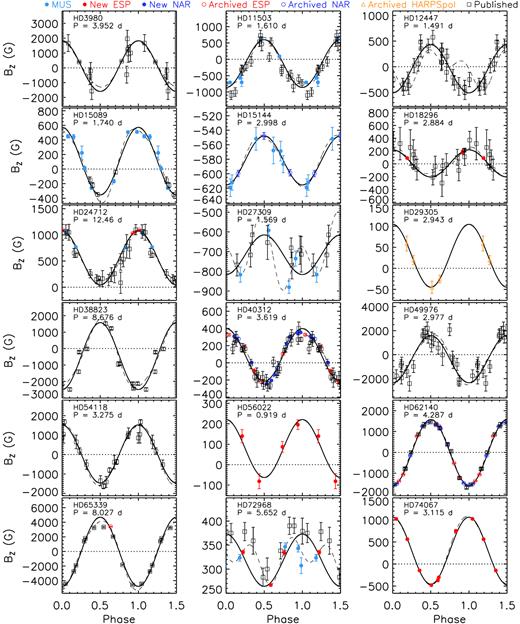
The 〈Bz〉 measurements used in this analysis phased according to each star’s rotational period – only those mCP stars with known Prot values are shown. The solid black curves and dashed black curves correspond to the best first- and second-order sinusoidal fits (defined by equation 1). Note that the periods listed in each figure are rounded and do not correspond to the actual Prot precision.
4.5 HD 148898
Manfroid, Mathys & Heck (1985) report three plausible rotational periods for HD 148898: 1.79 ± 0.02, 2.33 ± 0.02, and |$4.67\pm 0.08\, {\rm d}$|. Based on near-infrared variability, Catalano et al. (1998) adopted the value of |$P_{\rm rot}=0.7462(2)\, {\rm d}$| reported by Renson & Maitzen (1978). We obtained four new ESPaDOnS Stokes V observations for this star, which we combined with the single measurement published by Kochukhov & Bagnulo (2006). The five high-precision 〈Bz〉 measurements could not be adequately phased using |$P_{\rm rot}=1.79\pm 0.02\, {\rm d}$| (|$\chi ^2_{\rm red}=38$|); the 0.7462, 2.33, and |$4.67\, {\rm d}$| periods yield high-quality first-order sinusoidal fits (|$\chi ^2_{\rm red}\lt 0.01$|) and are consistent with the derived radii and vsin i (i.e. veq > vsin i for both periods). Here, we adopt |$P_{\rm rot}=2.3205(2)\, {\rm d}$| based on the marginally lower χ2 value associated with both the 〈Bz〉 and Hipparcos measurements compared to the longer |$4.682(1)\, {\rm d}$| period; however, we emphasize that additional observations are required to more confidently identify the correct Prot.
4.6 HD 151199
We only found one Prot value of HD 151199 reported in the literature: Gokkaya (1970) find that the star exhibits Ca ii K line variations having a period of |$6.143\, {\rm d}$|. The 〈Bz〉 measurements exhibit a number of statistically significant periods with none appearing within |$0.3\, {\rm d}$| of |$6.143\, {\rm d}$|. The vsin i value and stellar radius derived in Paper I imply a maximum Prot of approximately |$2.4\, {\rm d}$|. We adopt the minimal χ2 period within |$0.4\!-\!2.5\, {\rm d}$| (|$P_{\rm rot}=1.83317(22)\, {\rm d}$| and |$\chi ^2_{\rm red}=1.0$|); however additional magnetic, spectroscopic, or photometric measurements are required to verify this value due to the number of periods which yield reasonably high-quality sinusoidal fits.
4.7 HD 221760
Four high-precision Stokes V observations of HD 221760 were obtained with ESPaDOnS; the associated 〈Bz〉 measurements were found to vary from −72 ± 9 to |$57\pm 9\, {\rm G}$|. The period search analysis performed using the first-order sinusoidal function yielded a large number of statistically significant periods. None of the possible periods were found to be consistent with the |$12\!-\!13\, {\rm d}$| rotational periods suggested by van Genderen (1971) and Catalano et al. (1998) based on their detections of photometric variability. Furthermore, the vsin i value of |$22.4\pm 0.7\, {\rm km\, s^{-1}}$| and stellar radius of |$3.6\pm 0.3\, R_\odot$| derived in Paper I imply a maximum rotational period of |${\approx }9.1\, {\rm d}$|. We find that the 〈Bz〉 measurements are coherently phased by a period that is one-half that of one of the possible periods reported by Catalano et al. (1998) (|$P=12.665\, {\rm d}/2=6.3325\, {\rm d}$|).
While no additional archived Stokes V observations or published 〈Bz〉 measurements with sufficiently high precision could be found, 21 archived Stokes I HARPS observations are available . We attempted to obtain additional constraints on HD 221760’s Prot by searching for spectral line variability using the combined HARPS and ESPaDOnS Stokes I observations. No significant line profile variability could be detected (either visually or from equivalent width calculations) from various lines including those associated with Ti, Cr, and Fe.
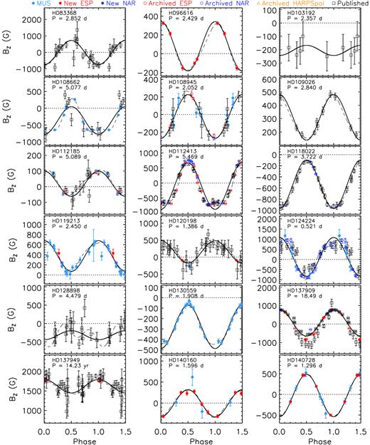
Continued from Fig. 2.
We adopt |$P_{\rm rot}=5.98\pm 0.06\, {\rm d}$| based on the preceding discussion, however, we emphasize that further confirmation of this value is required.
4.8 HD 64486, HD 117025, HD 176232, and HD 217522
No published rotational periods were found for these five mCP stars. We were unable to infer the Prot values of HD 64486, HD 117025, or HD 217522 on account of (1) an insufficient number of available 〈Bz〉 measurements and (2) the absence of any statistically significant variability in the associated Hipparcos photometric measurements. Prot of HD 176232 could not be derived on account of insufficient phase coverage of its very long rotational period: the available 〈Bz〉 measurements exhibit an approximately linear decrease from 400 to |$240\, {\rm G}$| over a |$12\, {\rm yr}$| period. The 〈Bz〉 measurements as a function of HJD are shown in Fig. 5 (aside from HD 217522, for which only a single measurement was obtained).
4.9 Distribution of rotational periods
In Fig. 7, we show the distribution of rotational periods for those 48/52 stars with known values. It is evident that the sample consists of mCP stars exhibiting minimum and maximum periods that are comparable to the known fastest rotators (|${\sim }0.5\, {\rm d}$|, e.g. Oksala et al. 2010; Grunhut et al. 2012) and slowest rotators (|${\gtrsim }100\, {\rm yr}$|, e.g. Mathys 2015). We find that the distribution is consistent with a lognormal distribution (demonstrated by the derived Kolmogorov–Smirnov (KS) test statistic of 0.15 ± 0.25). Fitting a Gaussian function to the distribution yields a mean of 3.1 ± 2.2. We note that there exists a tail to very long periods, with the longest determined period in our sample being |$97\, {\rm yr}$|.
We compared the distribution’s peak Prot with that yielded by larger previously published surveys. In fig. 8 of Wolff (1975), the distribution of compiled rotational periods is concentrated below |$10\, {\rm d}$| and exhibits a peak at |$P_{\rm rot}\lt 3.2\, {\rm d}$|; applying the same binning (|$\log {(\sigma _{P_{\rm rot}}/{\rm d})}=0.5$|) to the periods associated with the volume-limited survey yields the same peak location and sharp decline in the number of stars with |$P_{\rm rot}\gt 10\, {\rm d}$|. More recently, Netopil et al. (2017) reported rotational periods of more than 500 confirmed or candidate mCP stars. We derived a mean of |$2.4\, {\rm d}$| by fitting a Gaussian function to their distribution of reported periods; therefore, the two distributions’ peak locations are in agreement within the estimated uncertainty. The preceeding discussion suggests that, in terms of the rotational periods, the survey presented here is representative of the larger population of known mCP stars.
4.10 Inclination angles
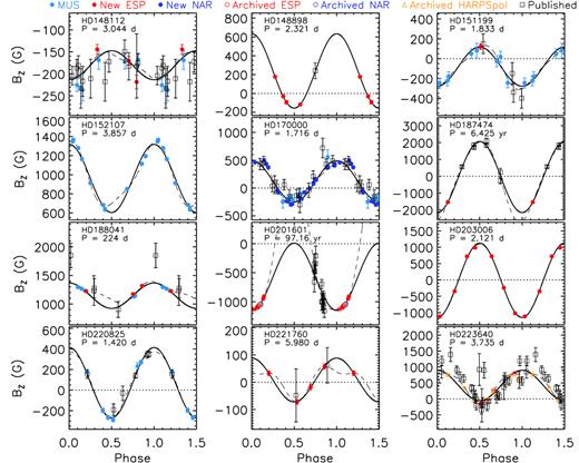
Continued from Fig. 3.
In Fig. 8 (top), we show the distribution of the 45 known inclination angles. It is apparent that the distribution is strongly peaked at the 45° < i < 60° bin. Such a feature is not associated with a distribution of inclination angles that are randomly oriented in space, which is characterized by a monotonic increase in frequency from 0° to 90°. Furthermore, either an excess of moderate i values (30° < i < 60°) or a deficiency of high i values (i > 60°) relative to a random distribution is apparent when comparing the cumulative distribution functions (CDFs) of sin i as shown in Fig. 8 (bottom). We computed a KS test statistic comparing the distribution of i values with that associated with a random distribution (0.19 ± 0.17), which suggests that the inclination angles of the mCP stars in this sample may not be drawn from a random distribution.
Previous studies have addressed the question of whether the inclination angles of mCP stars are in fact randomly oriented in space. Abt (2001) and Netopil et al. (2017) compiled 102 and 180 inclination angles, respectively, and concluded that the resulting distributions are consistent with random distributions. The discrepancy between the observed and expected (random) i distributions in the volume-limited survey presented here may be caused by the fact that the observed distribution is incomplete: for 7/52 stars, i could not be derived or found in the literature. We attempted to estimate the statistical significance of the 0.19 ± 0.17 KS test statistic by carrying out a Monte Carlo (MC) simulation. This involved generating 105 simulated distributions consisting of 45 i values sampled from the theoretical random distribution. KS test statistics comparing each simulated distribution with the theoretical random distribution were then calculated. We found that 7 per cent of the simulated distributions exhibited a test statistic ≥0.19; therefore, we conclude that the difference between the observed and random distributions is not statistically significant.
Although it is likely that the inclination angles presented here are randomly oriented, we note that the location of the maximum incidence of i shown in Fig. 8 is similar to the location of the distribution’s peak found in the results of the larger Abt (2001) and Netopil et al. (2017) studies. In fig. 1 of Abt (2001), the sin i distribution peaks at ≈0.7 (i ≈ 45°), while the inclination angles compiled by Netopil et al. (2017) exhibit a maximum frequency within 45° < i < 60°. This may not be entirely unexpected considering that a number of common mCP stars are included in all three studies: 20 and 21 per cent of the Abt (2001) and Netopil et al. (2017) samples of mCP stars with known i are also included in our volume-limited survey. The statistical significance of the position of this peak in our sample was estimated using the results of the MC simulation discussed above. For each of the 105 simulated distributions consisting of 45 randomly oriented i values, we determined the location of the maximum incidence when the distribution is binned using Δi = 15°, as shown in Fig. 8. Nineteen per cent of the simulated distributions exhibited a maximum incidence within 45° < i < 60° suggesting that the location of the peak is not statistically significant. We also evaluated the statistical significance of the peak height relative to the neighbouring bins (e.g. the peak shown in Fig. 8 exhibits a peak height of nine relative to the two neighbouring bins). We found that 7 per cent of the simulated distributions exhibited peaks with relative heights ≥9. Therefore, while the significance of the peak height is higher than that associated with its location, we do not consider it to be statistically significant.
5 MAGNETIC PARAMETERS
The magnetic field strengths and geometries of the mCP stars can be estimated using the ORM (Stibbs 1950). In particular, we use equations (1) and (2) of Preston (1967) to derive the strength of the field’s dipole component (Bd) along with the associated obliquity angle (β, i.e. the angle between the dipole component’s axis of symmetry and the star’s rotational axis). This derivation depends on the star’s inclination angle (i), linear limb-darkening coefficient (u), and ratio of the minimum to maximum longitudinal field strengths (r ≡ 〈Bz〉min/〈Bz〉max).
Linear limb-darkening coefficients were derived using the grid calculated by Díaz-Cordovés, Claret & Gimenez (1995). This grid is calculated for a range of surface gravities (|$0.0\le \log {g}\le 5.0\, {\rm [cgs]}$|), effective temperatures (|$3500\le T_{\rm eff}\le 50\, 000\, {\rm K}$|), and photometric filters (Johnson UVB and Strömgren uvby). We used the limb-darkening coefficients calculated for the Johnson V filter because of the fact that this filter’s transmission function approximately spans the wavelength range of the LSD line masks (|$3000\le \lambda \le 7000\, {\rm \mathring{\rm A} }$|) discussed in Section 3.1. The grid of Johnson V limb-darkening coefficients was interpolated for each star over log g and Teff (using the log g and Teff values derived in Paper I).
The ratios of minimum to maximum field strengths (r) for each star were derived from the fits to the phased 〈Bz〉 measurements shown in Figs 2–4. Both 〈Bz〉min and 〈Bz〉max were calculated using the mean (B0 ≡ C0) and amplitudes (B1 ≡ C1) associated with the first-order sinusoidal fits [i.e. equation (1) with C2 ≡ 0]. The uncertainties in B0 and B1 (and thus, in r) were derived by applying the method of residual bootstrapping. The method involves calculating the residuals associated with the 〈Bz〉 measurements and the (first order) sinusoidal fit. For each 〈Bz〉 measurement, we add to it a randomly selected residual and the sinusoidal fit is recalculated. This process is repeated |$10\, 000$| times yielding approximately Gaussian fitting parameter distributions, which are used to estimate 3σ uncertainties.
Finally, Bd and β were derived using the calculated values of i, u, and r according to equations (1) and (2) of Preston (1967). Given the number of parameters involved in this derivation (e.g. Teff, R, vsin i, etc.), it is difficult to evaluate how they are correlated. Without accounting for these correlations, the uncertainties in Bd and β will likely be erroneously low. We estimated |$\sigma _{B_{\rm d}}$| and σβ by extending the MC uncertainty analysis carried out in Paper I. This involved calculating each star’s Bd and β for ≳1000 data points each consisting of randomly selected effective temperatures and luminosities normally distributed according to their most probable values and their uncertainties (Shultz et al., in preparation; a brief description is presented in Paper I) . This analysis was extended by assigning vsin i and r values – randomly generated from normal distributions with widths defined by σvsin i and σr – to each of the previously generated MC data points. Ultimately, this method yields distributions of Bd and β values, which can be used to infer |$\sigma _{B_{\rm d}}$| and σβ. In general, the resulting distributions are either positively or negatively skewed. Therefore, rather than defining |$\sigma _{B_{\rm d}}$| and σβ using each distribution’s standard deviation, we adopt minimum and maximum limits defined such that 99.7 per cent of the distribution is enclosed.
In six cases (HD 3980, HD 38823, HD 108662, HD 108945, HD 137909, and HD 223640) the most probable vsin i values derived in Paper I were found to exceed the equatorial velocities (veq) calculated using Prot, and R; however, the vsin i and veq values of all six stars were found to be equal within the estimated uncertainties (i.e. they are consistent with i ≈ 90°). In these cases, we removed those MC data points for which vsin i > veq. The peak values of the resulting MC distributions were then used to define new, most probable vsin i values.
5.1 Dipole field strengths
In Fig. 9, we show the derived dipole field strengths for 45/52 mCP stars in the sample (i.e. those with known rotational periods and inclination angles and for which multiple 〈Bz〉 measurements are available). The Bd distribution is well characterized by a lognormal distribution as demonstrated by the derived KS test statistic of 0.10 ± 0.19. Fitting a Gaussian function to log (Bd/G) yields a mean and 3σ uncertainty of 3.4 ± 0.2 (corresponding to |$2.6^{+1.9}_{-1.1}\, {\rm kG}$|). The maximum derived Bd in the sample corresponds to |$18.1_{-2.7}^{+3.4}\, {\rm kG}$| (HD 65339), which is in agreement with the value reported by Landstreet (1988). The minimum derived Bd corresponds to |$330_{-60}^{+80}\, {\rm G}$| (HD 112185); however, the minimum dipole field strength derived when considering the upper Bd error limits corresponds to |$B_{\rm d}^{\rm max}=390\, {\rm G}$| (HD 221760).
The survey carried out by Aurière et al. (2007) was specifically designed to search for mCP stars hosting weak dipole fields. They reported a minimum most probable field strength (i.e. minimum Bd without considering the estimated lower error limits) of |$100\, {\rm G}$|. The minimum |$B_{\rm d}^{\rm max}$| found in their study is |$477\, {\rm G}$|, which is slightly higher but still comparable to that derived here. The fact that they did not find any dipole field strengths |${\lesssim }100\, {\rm G}$| led them to propose the existence of a critical dipole field strength (Bc), which defines a minimum field strength necessary for a field to maintain stability. They estimate that |$B_{\rm c}\approx 300\, {\rm G}$| for a typical A-type star and is indicated in Fig. 9; it is clear that the majority of the 45 Bd values derived for the stars in our volume-limited survey greatly exceed |$300\, {\rm G}$|.
The derivation of Bc by Aurière et al. (2007) applies to all A-type stars spanning the MS. Therefore, an additional test of the existence of Bc can be carried out by estimating each mCP stars’ Bd/Bc value as a function of fractional MS age (τ) and determining if Bd/Bc ≪ 1 at any point during its evolution across the MS. We estimated each stars’ R(τ) and Teff(τ) by interpolating evolutionary tracks computed by Ekström et al. (2012) and Mowlavi et al. (2012), which is discussed more thoroughly in Paper I. The change in Prot occurring across the MS was estimated using two grids of rotating evolutionary tracks. For stars with masses |$\lt 1.7\, M_\odot$|, we used the rotating solar metallicity (Z = 0.014) evolutionary tracks computed by Ekström et al. (2012) for veq/vc equal to 0.0 and 0.4 where veq and vc are the equatorial velocity and critical breakup rotational velocity at the zero-age MS (ZAMS). For stars with masses |$\ge 1.7\, M_\odot$|, we used the higher veq/vc density (veq/vc = 0.0, 0.1, 0.3, 0.5, 0.6, 0.7, 0.9, and 1.0) solar metallicity grids computed by Georgy et al. (2013). The change in the dipole field strength was estimated by assuming that magnetic flux is conserved. Under this assumption, Bd decreases with R−2 as R increases from the ZAMS to the terminal age MS (TAMS). We find that the predicted Bd/Bc values decrease monotonically along the MS; as a result, only one of the 45 stars with derived Bd values is predicted to have Bd/Bc < 1 at earlier points during its MS lifetime. The distributions of the observed Bd/Bc and the Bd/Bc values predicted at the ZAMS are shown in Fig. 10.
It is evident that both of the observed and predicted ZAMS Bd/Bc distributions shown in Fig. 10 exhibit a sharp decrease in frequency at Bd/Bc < 1. This is consistent with the notion that the current Bd/Bc values are initially drawn from a wider distribution containing lower Bd/Bc values: the initial distribution is truncated at Bd/Bc = 1 resulting in a sharp decline towards lower values.
5.2 Obliquity angles
In Fig. 11, we show the distribution and CDF associated with the 45 obliquity angles (β) derived using equation (3) of Preston (1967). The β distribution exhibits a moderate increase from low to high β values, which is qualitatively similar to that associated with a distribution of randomly oriented axes. A more quantitative comparison was carried out using the CDFs of the derived sin β and theoretical random distributions. We derived a KS test statistic of 0.17 ± 0.15 suggesting that the β values may not be randomly oriented. The significance of this KS test statistic was evaluated using the same MC simulation that was carried out in Section 4.10 with the inclination angles. The 105 simulated distributions were generated, each consisting of 45 β values drawn from the theoretical random distribution. A KS test statistic comparing each of the simulated random distributions with the theoretical random distribution were calculated. We found that 13 per cent of the resulting KS values were ≥0.17; therefore, we conclude that the apparent difference between the derived β values and the theoretical random distribution is statistically insignificant.
The inclination angles and magnetic parameters of the 52 confirmed mCP stars are listed in Table 4.
6 EVOLUTION OF MAGNETIC FIELD STRENGTH
In Paper I, we identified statistically significant trends in the average surface chemical abundances of certain elements (e.g. Si, Ti, Cr, and Fe) as functions of stellar age. Similar correlations between the atmospheric chemical abundances and ages of Bp stars have been previously reported by Bailey, Landstreet & Bagnulo (2014). The authors also found that the same elements exhibiting coherent changes with age also exhibit changes with the measured magnetic field strengths; this is attributed to a decrease in field strength with age as previously reported by Landstreet et al. (2007, 2008) for both MS Ap and Bp stars (|$8\lt T_{\rm eff}\lt 20\, {\rm kK}$|).
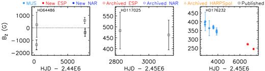
The 〈Bz〉 measurements used in this analysis associated with those stars with >1 measurement and without known Prot values.
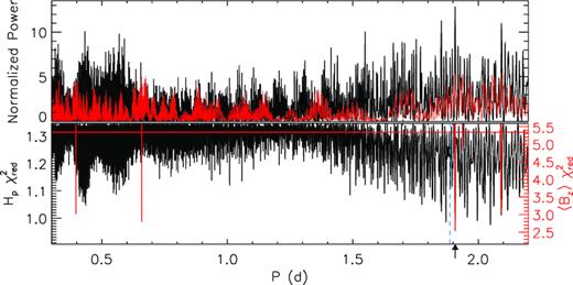
Normalized Lomb–Scargle periodograms (top) and χ2 distributions derived using the first-order sinusoidal function (bottom) associated with the Hipparcos (black) and 〈Bz〉 (red) measurements associated with HD 130559. The horizontal dotted–dashed red line corresponds to the 〈Bz〉 3σ confidence limit calculated with respect to |$\chi ^2_{\rm min}$|; the Hp periods shown in the χ2 distribution exhibit confidence limits <0.1σ. The black arrow indicates the adopted |$P_{\rm rot}=1.90798(71)\, {\rm d}$|. The vertical dashed blue line appearing in the χ2 plot corresponds to the |$1.8871(8)\, {\rm d}$| period identified by Wraight et al. (2012) based on STEREO photometry, which is not consistent with the 〈Bz〉 measurements.
In Fig. 12, we plot R, Bd, and BdR2 (i.e. the surface magnetic flux) as functions of age (log t/yr) and fractional MS age (τ). The 45 mCP stars represented in the figure are divided into low-mass (M/M⊙ < 2), intermediate-mass (2 ≤ M/M⊙ < 3), and high-mass (M/M⊙ ≥ 3) ranges. This is done for two reasons: (1) the increase in R as each star evolves across the MS increases with mass; and (2) the width of the MS spanned by each of the three mass ranges decreases with decreasing mass. Therefore, under the assumption that magnetic flux is conserved, we expect to see larger changes in Bd with age in the high-mass range compared to the low-mass range. This can result in an increase in the dispersion of Bd and BdR2 with increasing τ thereby decreasing our ability to detect such evolutionary changes.
The best-fitting linear functions were derived for each of the Bd and BdR2 values associated with the three mass intervals. We used an unweighted least-squares analysis because of the fact that the errors associated with Bd, log t/yr, and τ are typically large and asymmetric: Bd diverges as |i − β| → 90°, while log t/yr and τ are significantly more uncertain closer to the ZAMS than to the TAMS (e.g. see fig. 4 of Kochukhov & Bagnulo 2006). We found that the resulting fits yielded lower residuals compared to those obtained by considering both x and y uncertainties (e.g. using the method described by Williams, Bureau & Cappellari 2010). We estimated 1σ uncertainties in the fitting parameters by bootstrapping the residuals. The resulting linear fits are shown in Fig. 12 and the slopes are listed in Table 5.
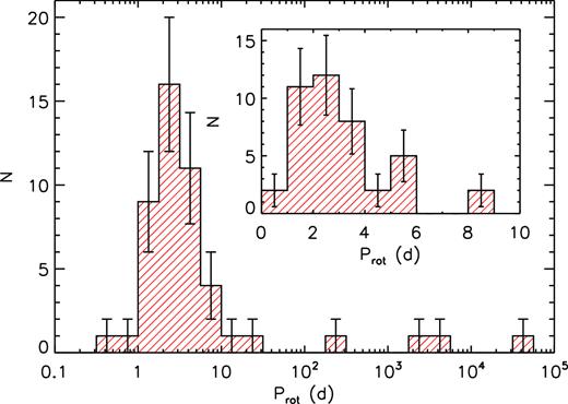
Distribution of rotational periods for 48/52 of the mCP stars. The inset plot shows the same distribution for |$P_{\rm rot}\le 10\, {\rm d}$|.
We find that the dipole field strengths associated with all three of the mass intervals decrease over both log t/yr and τ; we do not detect any changes in the magnetic flux (BdR2) with stellar age. We note that the uncertainties in R are relatively small (≲ 15 per cent) and that the estimated uncertainties in the slopes associated with Bd and BdR2 are comparable (particularly for the slopes involving τ). This suggests that the apparent differences in the rates of change of the field strength and the magnetic flux are not related to the uncertainty introduced by R. Therefore, we conclude that these results are statistically consistent with the notion that magnetic flux is conserved as an mCP star evolves across the MS.
The fact that Bd appears to decrease with increasing stellar age is qualitatively consistent with the findings of Landstreet et al. (2007), whose survey only consisted of cluster members with well-constrained ages. Moreover, the rate of field strength decline that they derived for stars having 3 ≤ M/M⊙ ≤ 4 (−0.42 ± 0.14) is consistent with that derived here for our sample’s high-mass stars (−0.89 ± 0.40). This agreement provides evidence in support of the notion that the magnetic fields of MS mCP stars decay with age. The rate of change of magnetic flux for the same mass intervals are also in agreement within the uncertainties: Landstreet et al. (2007) derived a slope of −0.22 ± 0.14 while we obtained −0.04 ± 0.42. Despite the quantitative agreement, it is noteworthy that Landstreet et al. (2007) detect a decrease in magnetic flux over time whereas, for our sample, we do not. It is clear that our sample includes significantly fewer high-mass stars (7 compared to 25) and that the derived ages have a much higher uncertainty. On the other hand, the Bd values associated with the majority of the stars in our sample have been derived from reasonably well-sampled 〈Bz〉 curves; for most of the stars included in the Landstreet et al. (2007) study, only single 〈Bz〉 measurements were obtained. The data set presented here can be used to assess the significance of this final point.
We carried out an MC simulation in which the magnetic field strengths of the stars in our sample were estimated using only a small number of randomly sampled 〈Bz〉 measurements. This involved generating 104 simulated data sets consisting of either 1 or 3 〈Bz〉 measurements for each of the 45 stars with known B0 and B1 (i.e. the mean and amplitude characterizing the 〈Bz〉 curves). The 〈Bz〉 measurements were generated using random phase values (θ ∈ [0, 1]) along with B0 and B1 such that 〈Bz〉(θ) = B0 + B1sin θ. Each star’s root-mean square field strength (Brms) was then calculated (as done by Landstreet et al. 2007). Finally, the linear fitting analyses involving log t/yr, Brms, and BrmsR2 were carried out and the derived slopes were compared with those generated using the original data set. In Fig. 13, we show the resulting distributions based on the BrmsR2 slopes.
The results of the MC simulation suggest that both the slopes of Brms and BrmsR2 as functions of log t/yr and τ are biased towards lower values when Brms is derived from a small number of 〈Bz〉 measurements. However, we find that the bias is small and decreases with increasing sample size. Considering the large sample size of the survey carried out by Landstreet et al. (2007), the bias is likely negligible as assumed by the authors. It is clear from the distributions shown in Fig. 13 that, depending on the number of 〈Bz〉 measurements used to derive Brms of each star, the uncertainty in the slope may be significantly affected. We note that the MC simulation uses the stellar ages derived for the current sample in Paper I; therefore, the results of the simulation are certainly affected by the large age uncertainties to some extent.
It is plausible that the lack of detection of flux decay in our sample could result from (1) a small sample size for each of the mass bins (in particular for the high-mass stars which are expected to exhibit the largest decrease) and (2) large errors in the stellar ages. Additionally, it is noted that, in terms of both log t/yr and τ, the mCP stars in our sample are generally older than those contained in the Landstreet et al. (2007) sample: the fraction of stars having τ < 0.4 is >50 per cent in the Landstreet et al. (2007) sample compared with 15 per cent in our volume-limited sample. In fig. 4 of Landstreet et al. (2008), it is apparent that the rate of flux decay associated with high-mass Ap stars is significantly higher for τ < 0.2 compared with τ > 0.2. This suggests that the apparent discrepancy in terms of the detection of flux decay between our sample and that of Landstreet et al. (2007) may be caused by a decay rate that is higher for younger MS stars coupled with the different age distribution of our sample.
7 DISCUSSION AND CONCLUSIONS
In Paper I, we presented an analysis of the fundamental properties and chemical abundances of 52 and 45 confirmed mCP stars, respectively, located within a distance of |$100\, {\rm pc}$|. This study is the first of its kind in two specific ways. First, it is focused on a volume-limited sample and thus, is less affected by the biases inherent to previous studies of samples of mCP stars (e.g. Kochukhov & Bagnulo 2006; Hubrig, North & Schöller 2007). Secondly, we have attempted to perform the analysis in a homogeneous manner such that any dispersion introduced by using varying techniques or theoretical models is minimized. The results presented here build on those of Paper I with the addition of an analysis of the confirmed mCP stars’ rotational periods and magnetic properties. In the following, we discuss these results and present our conclusions.
Rotational periods for 48/52 of the confirmed mCP stars in the sample were adopted based on (1) the available 〈Bz〉 measurements (i.e. newly obtained or unpublished measurements using ESPaDOnS, NARVAL, and MuSiCoS, newly analysed measurements, and previously published measurements) and (2) previously published values typically derived from photometric variability. In general, we found that the rotational periods inferred from magnetic measurements are consistent with the published values. However, in several cases Prot could not be identified ambiguously and we adopted Prot values based on somewhat unreliable or tenuous evidence (e.g. the newly obtained 〈Bz〉 measurements of HD 221760 were insufficient to derive a unique period and poor agreement was found with previously published values). Adopting unconfirmed rotational periods of certain stars in the sample may have contributed to the detection of an unusual and unexpected feature in the distribution of inclination angles.
The feature in question is the large peak i frequency occurring within 45°–60°, which also corresponds to the distribution’s global peak value. This is unexpected since it is not typically found in a distribution of i values that are randomly oriented in space (e.g. Abt 2001). Although statistically insignificant based on an estimated p-value of 0.07, it is perhaps noteworthy that a similar feature is found in the much larger data set of mCP i values published by Netopil et al. (2017). We note that the distribution shown in Fig. 8 is incomplete since the i values of 7/52 sample stars could not be derived; however, their inclusion is unlikely to dramatically reduce the feature’s statistical significance. No correlation between sin i and Galactic latitude is found (e.g. fig. 2 of Abt 2001), suggesting that the origin of the unexpected feature found in the i distribution is unlikely to be environmentally dependent.
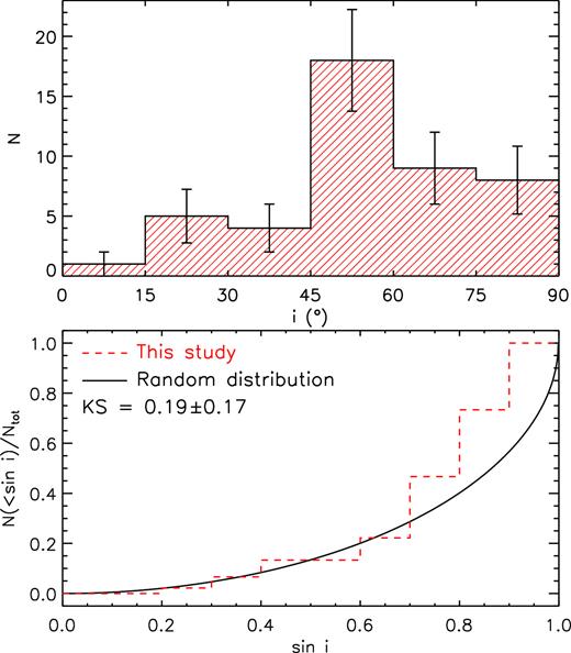
Top: distribution of inclination angles for the 44/52 mCP stars with known vsin i and known Prot values or with published i values. Bottom: CDF of sin i (dashed red) compared against that associated with a distribution of randomly oriented rotational axes (solid black). The KS test statistic of KS = 0.19 ± 0.17 suggests that the inclination angles may not be distributed randomly.
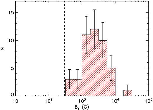
Distribution of dipole magnetic field strengths for 45/52 of the mCP stars. The vertical dashed line corresponds to the critical field strength of a typical MS A-type star (|$B_{\rm c}=300\, {\rm G}$|) estimated by Aurière et al. (2007).
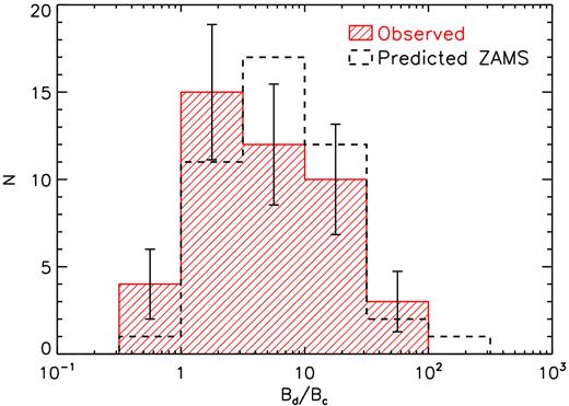
Distribution of the ratio of Bd to the critical field strength (Bc) derived by Aurière et al. (2007); these authors hypothesize that no A-type stars should be found exhibiting Bd/Bc < 1 (indicated by the vertical dashed line).
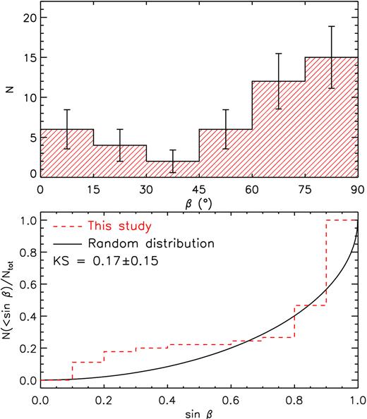
Top: distribution of obliquity angles for the 45/52 mCP stars with known Prot and i values and for which multiple 〈Bz〉 measurements are. Bottom: CDF of sin β (dashed red) compared against that associated with a distribution of randomly oriented magnetic dipole axes (solid black). The KS test statistic of KS = 0.17 ± 0.15 suggests that the inclination angles may not be distributed randomly.
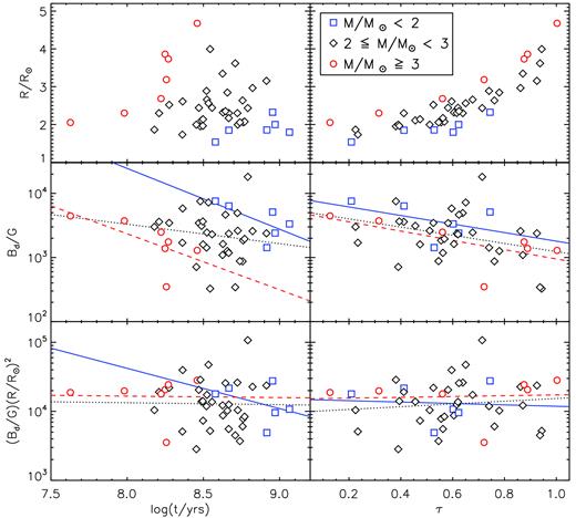
Radius (R, top row), dipole field strength (Bd, middle row), and BdR2 (bottom row) for 45/52 of the mCP stars in the sample as functions of logarithmic stellar age (log t/yr, left-hand column) and fractional MS age (τ, right-hand column). Three mass ranges are identified: M/M⊙ < 2, 2 ≤ M/M⊙ < 3, and M/M⊙ ≥ 3. The lines correspond to the best-fitting linear functions for the low-mass (solid blue), intermediate-mass (dotted black), and high-mass (dashed red) stars. The derived slopes and their uncertainties are listed in Table 5.
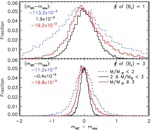
Distributions comparing the slope of BrmsR2 as a function of log t/yr generated from the MC simulated data sets with that generated from the original data set. The top distribution corresponds to the Brms values calculated using one randomly generated 〈Bz〉 measurement, while the bottom distribution uses three measurements. The mean values of each distribution (〈mMC − mobs〉) are listed in order of increasing mass.
Landstreet & Mathys (2000) derived β values for a sample of 24 Ap stars and found that the slow rotators (|$P_{\rm rot}\gt 25\, {\rm d}$|) tend to exhibit low β values, while only two faster rotators in their sample (|$P_{\rm rot}\lt 25\, {\rm d}$|) were found with β < 60°. Our sample consists of five stars with |$P_{\rm rot}\gt 25\, {\rm d}$|; only one of these stars was assigned a value of β (obtained by Landstreet & Mathys 2000). Obliquity angles were derived for all 44 of the stars with |$P_{\rm rot}\lt 25\, {\rm d}$|. We did not identify any clear correlations between β and Prot. We do confirm the findings of Landstreet & Mathys (2000) that β tends to be large for these more rapidly rotating stars (i.e. those with Prot values that are more commonly found amongst mCP stars e.g. Wolff 1975; Bychkov, Bychkova & Madej 2005; Netopil et al. 2017). However, we find that the distribution of β values is consistent with a theoretical distribution of randomly oriented axes. We also did not find any clear correlations between β and absolute stellar age or fractional MS age or between β and Bd. Therefore, we find no evidence that the β values of stars with |$P_{\rm rot}\lt 25\, {\rm d}$| are preferentially oriented as a result of some physical mechanism (e.g. Mestel & Takhar 1972; Moss 1984). We note that this result is consistent with the findings of Wade (1997) who identified both young and evolved mCP stars that exhibit moderate β values (∼30°).
We were able to constrain the dipole magnetic field strengths for 45/52 of the mCP stars in our sample. The minimum field strength found in our sample when considering the upper error limits of Bd corresponds to |$390\, {\rm G}$|. The fact that we did not find any stars with fields |${\lesssim }100\, {\rm G}$| is consistent with the notion that there exists a magnetic desert (e.g. Aurière et al. 2007; Lignières et al. 2014). We also derived the critical field strengths of each of the stars, which corresponds to the minimum field strength required for an mCP star’s field to remain stable as hypothesized by Aurière et al. (2007). Three stars (HD 29305, HD 56022, and HD 112185) were found exhibiting upper error limits of Bd/Bc < 1; however, no stars were found having Bd/Bc ≪ 1. These stars may serve as useful targets for constraining Bc, if this critical lower field strength limit does exist.
Although our volume-limited sample does not contain any examples of mCP stars with field strengths well below Bc, several examples of intermediate- and high-mass stars have recently been reported. Fossati et al. (2015) derived a dipole field strength of |$60\lt B_{\rm d}\lt 230\, {\rm G}$| for the massive B1 II/III star, β CMa, suggesting that the magnetic desert feature may be limited to the cooler, intermediate-mass stars studied by Aurière et al. (2007). On the other hand, Alecian et al. (2016) report a field strength of |$B_{\rm d}=65\pm 20\, {\rm G}$| for an Ap star with an effective temperature estimated to be |$11.4\pm 0.3\, {\rm kK}$|. This star is the primary component of the spectroscopic binary, HD 5550, which exhibits an orbital period |${\sim }6.8\, {\rm d}$|. They find that the magnetic component likely rotates with a period of |$6.8\, {\rm d}$|; no radius or luminosity is reported. Assuming that the star is positioned somewhere on the MS, we obtain a rough estimate of the critical field strength (equation 3) of |$130\lesssim B_{\rm c}\lesssim 220\, {\rm G}$|; therefore, it is likely that Bd/Bc < 1. It is possible that the fact that this star is in a binary system with a relatively short period may somehow influence this result, however, considering the |$\gt 5\, {\rm d}$| orbital period, it is unlikely that any tidal interactions are taking place. It is also possible that the order of magnitude estimate of Bc estimated by Aurière et al. (2007) is simply too high or is in need of refinement.
A clear increase in the incidence rate of mCP stars with increasing mass was identified in Paper I (mCP stars account for ≈3 per cent of MS stars with |$M\approx 1.5\, M_\odot$| and ≈10 per cent of MS stars with 3.0 < M/M⊙ < 3.8). The MC simulation involving the Zorec & Royer (2012) data did not reveal an increase in Bc with decreasing M, which might have otherwise explained the increased rarity of lower mass mCP stars. We conclude that, regardless of whether Bc exists, this particular property of mCP stars is likely a product of additional factors such as the increase in subsurface convection zone depth with decreasing mass.
In Paper I, we detected the decrease of average surface abundances of certain elements such as Si, Ti, and Fe over stellar age similar to the trends reported by Bailey et al. (2014) for Bp stars. Here, we detect a decrease in Bd over both absolute age and fractional MS age. The rate of Bd decrease is strongest for the highest mass stars in our sample and is found to be in agreement with that reported by Landstreet et al. (2007) based on Brms values. Contrary to the findings reported by Landstreet et al. (2007), we do not detect any change in the surface magnetic flux over time; however, the reported decay rates are in agreement within the adopted uncertainties. We conclude that the lack of detection of surface flux decreases can plausibly be attributed to our smaller sample size and lower age precision.
SUPPORTING INFORMATION
Table 1. Observations of confirmed mCP stars – those stars for which at least one definite detection was obtained based on the criterion proposed by Donati et al. (1997).
Figure S1. Examples of LSD profiles at one or two rotational phases.
Figure S2. Continued from Fig. S1.
Figure S3. Continued from Fig. S2.
Figure S4. Continued from Fig. S3.
Figure S5. Continued from Fig. S4.
Figure S6. Continued from Fig. S5.
Figure S7. The Hipparcos Epoch Photometry associated with those mCP stars with known Prot.
Figure S8. Continued from Fig. S7.
Figure S9. Continued from Fig. S8.
Figure S10. The Hipparcos Epoch Photometry associated with those stars without known Prot values.
Please note: Oxford University Press is not responsible for the content or functionality of any supporting materials supplied by the authors. Any queries (other than missing material) should be directed to the corresponding author for the article.
ACKNOWLEDGEMENTS
GAW acknowledges support in the form of a Discovery Grant from the Natural Science and Engineering Research Council (NSERC) of Canada.
