


ABSTRACT
We present a detailed description and validation of our massively parallel update to the mass-Peak Patch method, a fully predictive initial-space algorithm to quickly generate dark matter halo catalogues in very large cosmological volumes. We perform an extensive systematic comparison to a suite of N-body simulations covering a broad range of redshifts and simulation resolutions, and find that, without any parameter fitting, our method is able to generally reproduce N-body results while typically using over 3 orders of magnitude less CPU time, and a fraction of the memory cost. Instead of calculating the full non-linear gravitational collapse determined by an N-body simulation, the mass-Peak Patch method finds an overcomplete set of just-collapsed structures around a hierarchy of density-peak points by coarse-grained (homogeneous) ellipsoidal dynamics. A complete set of mass peaks, or haloes, is then determined by exclusion of overlapping patches, and second-order Lagrangian displacements are used to move the haloes to their final positions and to give their flow velocities. Our results show that the mass-Peak Patch method is well suited for creating large ensembles of halo catalogues to mock cosmological surveys, and to aid in complex statistical interpretations of cosmological models.
1 INTRODUCTION
Future large-scale structure and cosmic microwave background (CMB) surveys require extensive ensembles of large-volume mock halo catalogues in order to model observables, estimate their covariance matrices, study their systematic errors, and test data analysis pipelines. Due to the size of these surveys, and the need to simulate many different cosmological parameter values and ‘beyond the standard model cosmologies’, this task becomes computationally restrictive when using traditional N-body methods to generate halo catalogues. Therefore, accelerated methods for generating simulations of the large-scale structure of the universe are widely desired in cosmology, and this has resulted in an introduction of many ‘approximate’ methods over the last few decades. Each of these methods is built upon different approximations to the fully non-linear gravitational collapse calculated by an N-body simulation, and many use fit parameters calibrated to the N-body results. Our focus here is on the mass-Peak Patch (mPP) method of Bond & Myers (1996a,b,c), the natural outgrowth of the ‘peaks’ picture of Bardeen et al. (1986) and the excursion set picture of Bond et al. (1991), augmented by the fundamental recognition of the role of tides and strain in defining dynamical evolution in the cosmic web. Approximate methods can be divided into three main groups: stochastic, abridged particle mesh, and predictive.
Stochastic methods such as EZMOCKS (Chuang et al. 2015a), HALOGEN (Avila et al. 2015), PATCHY (Kitaura, Yepes & Prada 2014), PThaloes (Scoccimarro & Sheth 2002; Manera et al. 2013), QPM (White, Tinker & McBride 2014), and lognormal models (Coles & Jones 1991; Agrawal et al. 2017), apply a (usually stochastic) model to a density field in order to lay down haloes or galaxies, commonly based on free parameters fit to N-body results. Though fast, they require calibration, and have difficulty extending to regimes (cosmology, redshifts, or higher point estimators) where they have not already been fit (Colavincenzo et al. 2018).
The second group, which includes COLA (Tassev, Zaldarriaga & Eisenstein 2013; Howlett, Manera & Percival 2015; Izard, Crocce & Fosalba 2016) and FastPM (Feng et al. 2016), can be considered as abridged particle mesh methods. These use additional approximations on top of standard particle-mesh gravity solvers to attempt to achieve accurate gravitational evolution with far fewer timesteps than required by a pure N-body, while still using standard N-body halo finding techniques. COLA uses the N-body solver to add a residual displacement on top of solutions from Lagrangian perturbation theory (LPT), while FastPM uses a broad-band correction applied at each time-step to artificially enforce the correct linear growth on large scales. These are very accurate for approximate methods, but still require ∼10–40 time-steps, halo finding, and can require a significant memory overhead.
The third group can be dubbed predictive methods, which the mPP method belongs to. Others in this class include PINOCCHIO (Monaco, Theuns & Taffoni 2002; Monaco et al. 2013) and HaloNet (Berger & Stein 2019). These methods implement physical models of gravitational collapse (or machine learned models in the case of HaloNet) to directly find haloes in the initial conditions, and then use a version of LPT to move them to their final positions.1 PINOCCHIO, the most similar to our Peak Patch method, computes collapse times of individual dark matter particles using an ellipsoidal collapse model based on LPT, and then applies a prescription to fragment the collapsed cells into distinct objects (haloes). This method still requires calibration to N-body simulations to determine free parameters in the fragmentation step.
The mPP method described and validated here explicitly models non-linear halo collapse and exclusion. As such, it requires essentially no additional calibration with respect to N-body simulations, as the basic ingredients of coarse-grained local ellipsoidal dynamics into the non-linear regime, hierarchical exclusion of small-scale entities within larger scale entities, and bulk motion and flow, are invariant. Radical variation of cosmological parameters does not alter the algorithm, nor does focusing on different halo definitions, selecting on secondary halo properties, or even choosing to concentrate on dynamical entities that are not haloes. This allows modular improvements to be straightforwardly incorporated, e.g. improving flow dynamics beyond second-order LPT [2LPT, such as Kitaura & Heß (2013) or Neyrinck (2016)], adding non-cold dark matter (non-CDM) forces to ellipsoidal dynamics, or extending to all manner of ‘beyond the standard model of cosmology’ situations. The mPP method also requires significantly less memory usage than abridged particle mesh methods, at a minimum (maximum) of 28 (84) bytes per particle, depending on if memory is the limiting step, compared to 120 bytes for FastPM and 144 bytes for COLA [when using an optimistic value of a force resolution factor, B = 2, and a no overallocation of memory storage (A = 1), which is in practice needed. Using routine values of B = 3 and A = 1.5 increases the memory requirements to 300 and 336 bytes per particle for FastPM and COLA, respectively] (Feng et al. 2016).
Many validation exercises have shown that the mPP method works well, beginning with the second of the original set of mPP papers, The Peak-Patch Picture of Cosmic Catalogs: II Validation (Bond & Myers 1996b), which used the then state-of-the-art 1283 adaptive particle mesh CDM (without Λ) simulations of Couchman (1991) and the first spherical overdensity halo finder to demonstrate with many statistical tests the accuracy of the Peak-Patch catalogues for the cluster-group system, including of the mass function and the spatial distribution. Further testing was done throughout the nineties, including on ΛCDM cosmology. The haloes in the mPP method, oriented according to the tidal field, were the basis of the theory of the cosmic web of Bond, Kofman & Pogosyan (1996).
Very recently, motivated by the mock simulation requirements for the Euclid mission (Laureijs et al. 2011), seven of the approximate methods, including mPP, were tested in detail in a set of three papers, comparing their clustering statistics and covariance matrices with those from N-body simulations constructed from the same initial conditions. Lippich et al. (2019) compared the correlation functions, Blot et al. (2018) compared the power spectrum multipoles, and Colavincenzo et al. (2018) compared the bispectra. These papers showed all the methods fared well, including the mPP method. For another recent performance comparison of approximate methods (not including mPP) see Chuang et al. (2015b), and for a detailed review of the subject see Monaco (2016). Though it may seem then that the mPP method has been validated in a modern as well as an ancient setting, these works were limited to a single redshift and simulation resolution. In this work, we expand upon these validations to multiple redshifts and simulation resolutions.
In Section 2, we present the updated and massively parallel version of the mPP method of Bond & Myers (1996a), highlighting and testing the inherent choices needed to run the large-scale simulations required for the mocks of current and future data. In Section 3, we validate mPP halo catalogues against those from a suite of N-body runs at various redshifts and simulation resolutions by comparing with a variety of summary statistics, including novel halo-proximity measures. In Section 4, we summarize our findings and discuss their implications along with the many important applications of the method already underway. Finally, in Appendix A, we discuss in detail the performance and parallelization scheme of the updated Peak Patch method.
2 THE MASS-PEAK PATCH METHOD
We generate halo catalogues with the mPP approach, originally described in Bond & Myers (1996a,b,c, hereafter referred to as BM), and recently used to create large synthetic mocks of the extragalactic microwave sky2 (Stein et al., in preparation), mocks of the carbon monoxide line emission from high-redshift galaxies (Tveit Ihle et al. 2018), and to create covariance matrices of clustering statistics (Lippich et al. 2019; Blot et al. 2018; Colavincenzo et al. 2018). In this new version, we have adapted the method to run on massively parallel computing architectures, and performed systematic studies of the accuracy and parameter choices required for application to large-scale structure surveys. Bond & Myers (1996a) provide the physical motivation and analytical derivations, while here we provide a brief summary of our new implementation and the parameters needed to run a given simulation.
The mPP method can be thought of as a dark matter halo finder that operates on the initial (Lagrangian) density field, which then uses LPT to displace the haloes to their final (Eulerian) positions. The gravitational collapse of haloes is approximated by solving the set of ordinary differential equations of homogeneous ellipsoid collapse, which depend only on the strain tensor of the linear displacements averaged over a corresponding spherical region in Lagrangian space. The four main steps of the method can be understood through Fig. 1 and are described in more detail in the following list:
- Generation of the initial overdensity field |$\delta (\boldsymbol {q}) = \frac{\rho (\boldsymbol {q}) - \overline{\rho }}{\overline{\rho }}$|, where |$\boldsymbol {q}$| is the initial (Lagrangian) position. This is accomplished by first generating a white noise field on a 3D lattice by drawing each lattice value from a Gaussian distribution with unit variance and a mean of 0, and then convolving with the linear matter power spectrum for the given cosmological parameters of the simulation. As the mPP method works on a discrete periodic cubic lattice, we perform many operations in the Fourier domain, where the Fourier transform of the matter overdensity field, |$\delta (\boldsymbol {k})$|, is defined throughThroughout this paper, we use the same notation for variables in either domain, and simply denote operations done in real space with the Lagrangian |$\boldsymbol {q}$| (or Eulerian |$\boldsymbol {x}$|) variable, and those done in Fourier space by the use of |$\boldsymbol {k}$|.(1)\begin{eqnarray*} \delta (\boldsymbol {q})= \frac{1}{(2 \pi)^3} \int \mathrm{ d}\boldsymbol {k}\ \mathrm{ e}^{i \boldsymbol {k}\cdot \boldsymbol {q}} \delta (\boldsymbol {k}) . \end{eqnarray*}The first- and second-order linear displacements, |$\boldsymbol {s}^{{(1)}}(\boldsymbol {q})$| and |${\boldsymbol {s}}^{{(2)}}(\boldsymbol {q})$|, are then calculated from the density field throughand(2)\begin{eqnarray*} \boldsymbol {s}^{{(1)}}(\boldsymbol {q})=\frac{D^{{(1)}}}{(2\pi)^3} \int \mathrm{ d}\boldsymbol {k}\ i \frac{\boldsymbol {k}}{k^2} \mathrm{ e}^{i \boldsymbol {k}\cdot \boldsymbol {q}} \delta (\boldsymbol {k}) \end{eqnarray*}(3)\begin{eqnarray*} {\boldsymbol {s}}^{{(2)}}(\boldsymbol {q}) =-\frac{D^{{(2)}}}{(2\pi)^3} \int \mathrm{ d}\boldsymbol {k}\ i \frac{\boldsymbol {k}}{k^2} \mathrm{ e}^{i \boldsymbol {k}\cdot \boldsymbol {q}} F(\boldsymbol {k}), \end{eqnarray*}|$\boldsymbol {s}^{{(1)}}_{\mathrm{ i,j}}(\boldsymbol {q})=\frac{\mathrm{ d}\boldsymbol {s}^{{(1)}}_\mathrm{ i}(\boldsymbol {q})}{\mathrm{ d}q_\mathrm{ j}}$| (so |$\boldsymbol {s}^{{(1)}}_{\mathrm{ i,j}}(\boldsymbol {k})=-k_\mathrm{ i}k_\mathrm{ j}\delta (\boldsymbol {k})/k^2$|), and D(1) and D(2) are the first- and second-order linear growth factor, respectively. By Fourier transforming to configuration space and performing the multiplications necessary sequentially, we are able to maintain the memory usage of the code at seven floats per mass element (|$\delta (\boldsymbol {q})$|, |$\boldsymbol {s}^{{(1)}}(\boldsymbol {q})$|, and |${\boldsymbol {s}}^{{(2)}}(\boldsymbol {q})$|) at the expense of only one additional Fourier transform. All fields are expressed in terms of their values at a redshift of 0.(4)\begin{eqnarray*} \mathrm{where}\ F(\boldsymbol {q})= \sum _{i\gt j}\big[\boldsymbol {s}^{{(1)}}_{\mathrm{ i,i}}(\boldsymbol {q})\boldsymbol {s}^{{(1)}}_{\mathrm{ j,j}}(\boldsymbol {q})- \boldsymbol {s}^{{(1)}}_{\mathrm{ i,j}}(\boldsymbol {q})\boldsymbol {s}^{{(1)}}_{\mathrm{ i,j}}(\boldsymbol {q})\big], \end{eqnarray*}
- The location of potential dark matter halo candidates are found by smoothing the density field on a number of filter scales, Rf, to find regions above a certain density threshold bywhere f denotes the type of filtering used (f = G → Gaussian, f = TH → top hat, etc.). The size (mass) of the halo is found by solving a set of homogeneous ellipsoidal collapse equations to determine if the given region will gravitationally collapse by the redshift in question. The collapse redshift is determined by the linear strain |$\overline{e}^{{(1)}}_{\mathrm{ ij}}\equiv (\partial {\overline{\boldsymbol {s}}^{{(1)}}_\mathrm{ i}}/\partial {q_\mathrm{ j}}+\partial {\overline{\boldsymbol {s}}^{{(1)}}_\mathrm{ j}}/\partial {q_\mathrm{ i}})/2$|, averaged over a sphere centred on each region of interest (see Section 2.1.2 for details).(5)\begin{eqnarray*} \delta (\boldsymbol {q};R_\mathrm{ f}) = \frac{1}{(2\pi)^3} \int \mathrm{ d}\boldsymbol {k}\ \mathrm{ e}^{i \boldsymbol {k}\cdot \boldsymbol {q}} \delta (\boldsymbol {k}) W_\mathrm{ f}(\boldsymbol {k}; R_\mathrm{ f}), \end{eqnarray*}
Overlapping regions of Lagrangian space belonging to multiple haloes are dealt with through exclusion, which can be of various physically motivated varieties as described in Section 2.1.3.
Haloes are then displaced to their final (Eulerian) position |$\boldsymbol {x}_\mathrm{ h}$|, at redshift |$z$|, using |$\boldsymbol {x}_\mathrm{ h}(z)=\boldsymbol {q}_\mathrm{ h} + D^{{(1)}}(z_\mathrm{ h})\overline{\boldsymbol {s}}^{{(1)}}+ D^{{(2)}}(z_\mathrm{ h})\overline{\boldsymbol {s}}^{{(2)}}$|, where |$\overline{\boldsymbol {s}}^{{(1)}}$| and |$\overline{\boldsymbol {s}}^{{(2)}}$| are the first- and second-order displacement fields averaged over the volume of the halo. We use the standard approximation |$D^{{(2)}}(z) = -\frac{3}{7}D(z)^2\Omega _\mathrm{ m}^{-1/143}$| (Bouchet et al. 1995). The velocity of each halo is determined by |$\mathbf {v}_\mathrm{ h}=a_\mathrm{ h}[\dot{D^{{(1)}}}(z_\mathrm{ h})\overline{\boldsymbol {s}}^{{(1)}}+\dot{D^{{(2)}}}(z_\mathrm{ h})\overline{\boldsymbol {s}}^{{(2)}}].$|
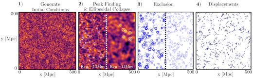
The four main steps of the mPP method. (1) Generation of a linear density field at |$z$| = 0. (2) Candidate halo locations (white circles, with a radius equal to the smoothing scale they were found at) are found by top-hat smoothing the linear density field on a hierarchy of filter scales and selecting density peaks above the threshold δc ∼ 1.5. The Lagrangian radius of the collapsed region (blue circles) is then determined by adjusting the radius until the non-linear ellipsoid trajectories, homogeneous over that radius in all three directions, have compactified to near-zero volume by the redshift in question. Haloes in a slice thickness equal to the filter size are shown, and the left (right) half of the image shows the result of smoothing with a top-hat filter size equal to 5.5 Mpc (13 Mpc). Note that some density peaks above the linear density threshold do not end up collapsing, a consequence of the role of tides and strain in the gravitational collapse of a halo. (3) Exclusion is performed to trim overlapping patches in order to create a final complete set of disconnected ordered mass peaks (haloes). The left-hand side of the image shows the full catalogue before exclusion, while on the right-hand side, we have performed exclusion. (4) Haloes are moved to their final positions using second-order LPT. Black arrows show the displacements from the initial positions, and the halo size shown is R200, M.
2.1 Optimal mass-Peak Patch parameters
Though we do not vary the free parameters of the mPP model with cosmology or resolution, and no parameters are fit to N-body simulations, there still remain a few definitions of halo collapse and exclusion parameters that need to be chosen in order to perform a simulation, and to maximize computational efficiency. These include the overdensity at which a halo is considered to have collapsed, how to divide overlapping volumes of Lagrangian space belonging to separate halo candidates in order to avoid double counting of mass, and how to efficiently find the locations of interest at which to calculate the ellipsoidal collapse equations. These choices are discussed and validated in the remainder of this section, and the optimal parameter findings settled upon are listed in Table 1.
Parameters of the mPP method that need to be specified in advance in order to run a simulation. Entries followed by a † are fundamental to the physical choice of approximating gravitational collapse used in the mPP method, while those without a † are simply to maximize computational efficiency.
| Algorithm step | Required parameters | Finalized choices |
|---|---|---|
| Density-peak finding (Section 2.1.1) | Type of filters | Top hat |
| Spacing between filters | Logarithmic in R or σ(R), or Linear in σ(R) | |
| Total number of filters | 20–30 | |
| Ellipsoidal collapse (Section 2.1.2) | Initial search radius | 1.75 Rf |
| Overdensity of a halo† | Δh = 200 |$\overline{\rho }_M$| | |
| Axis ‘freezeout’ ratio† | (λ3, λ2, λ1) = (|$\Delta _\mathrm{ h}^{-1/3}$|, |$\Delta _\mathrm{ h}^{-1/3}$|, 0.01) | |
| Exclusion (Section 2.1.3) | Partition of overlapping Lagrangian space† | Binary exclusion, type (ii) |
| Displacements | First- or second-order LPT | Second order |
2.1.1 Density-peak finding to generate candidate mass-peak points
The mPP method is a halo finder that identifies haloes with the largest regions of Lagrangian initial-state space that will collapse by the redshift in question using approximate dynamics, rather than the more exact N-body dynamics used for final-state Eulerian haloes. The first mPP step after the generation of the initial conditions is to generate a point process of possible sites of halo collapse. A highly overcomplete set is to use every initial-space lattice point, adjusting the Lagrangian radius of the region until the non-linear ellipsoid trajectories, homogeneous over that radius in all three directions, would have compactified to near-zero volume. In its fully glory, this is the correlated excursion set approach. Afterwards, the final complete set of non-overlapping haloes would be found by an exclusion process.
In practice, such dense sampling of candidates is a computationally expensive overkill. BM used a much smaller subset of linear density peaks smoothed on a hierarchy of filter scales {Rf}, chosen to lie above a linear density threshold δc low enough that it would not cause collapsed structures to be missed. The concrete choice δc ∼ 1.5 was made, safely below the δcrit = 1.686 of top-hat spherical overdensity collapse, and the catalogues were shown to be insensitive to the specific value chosen. We continue with that choice in our modernized version. Smoothing is performed by convolving the density field with a top-hat filter of the form |$W(kR_\mathrm{ f})=3j_1(\boldsymbol {k}R_\mathrm{ f})/(\boldsymbol {k}R_\mathrm{ f})$|, where j1 is the spherical Bessel function of order 1. This differs from the BM implementation in which Gaussian smoothing was used, since we found that this gives more candidate peak points on a given scale than Gaussian or sharp k-space filtering, and is better matched to how we actually average various fields about the candidate points to determine the ellipsoidal dynamics, namely with top-hat filtering over scales Rc. The number density of peaks on a coarse-grained scale Rf scales as |$R_\mathrm{ f}^{-3}$|, meaning the smallest filters in the hierarchy dominate the candidate peak list, so there is much room for modifying the distribution of filters without adding much more expense than that of the smallest element in the multiresolution hierarchy.
Thus, in order to optimize performance, we want to determine the best number of filters and their spacing for our ‘filter bank’. Too few filters may cause potential haloes in the simulation to be missed, while too many filters, especially of small scale, will reduce the computational performance of the code. The filters need to span a range that covers the mass range of haloes that we expect to find. The largest halo expected to be found at redshift |$z$| = 0 has a mass of |${\sim }10^{16}\, \mathrm{M}_\odot$|, corresponding to a radius of ∼36 Mpc in Lagrangian space, while the smallest halo is set by the resolution of the simulation. At a larger redshift, one can use a universal halo mass function to quickly estimate the size of the largest halo expected to be found (e.g. Tinker et al. 2008). For the homogeneous ellipsoidal calculations we use spherical averaging, which essentially imposes a minimum number of lattice sites needed for good smoothed-field resolution. Here, we set the minimum radius to be 2alatt, two lattice spacings of size alatt in the simulation (also called the cell size in this work). This therefore defines a minimum halo mass that we can possibly resolve: about each candidate point at least 32 neighbours are needed to encompass the top-hat smoothing estimates, similar to the minimum count used in smoothed particle hydrodynamic simulations. For more accurate sphericalization, a minimum count of 100 lattice ‘particles’ is more conservative, and is the typical number we use to define our minimum halo target mass in the simulations. The speed of the mPP method means that there is no real problem with making larger and larger lattices, so we can design a simulation to achieve a desired minimum resolved halo mass given a specified box size.
![To maximize the computational performance of the mPP method, we converged on an optimal ‘filter bank’ by running a suite of 10243 particle, 1024 Mpc simulations at $z$ = [0, 1, 2], which varied the number and spacing of filters. Each column (type of filter spacing) shows the convergence of the mPP mass function when varying the number of filters, referenced to the ‘converged’ case of 100 filters. From left to right, we present linear spacing in Rf, logarithmic spacing in Rf, linear spacing in σ(Rf), and logarithmic spacing in σ(Rf). Each row shows a different redshift, from $z$ = 2 at the top to $z$ = 0 at the bottom. Colours represent the number of filters used in each filter bank, where blue, red, and black indicate 10, 20, and 30 filters, respectively. Filters are spaced from a minimum size of Rmin = 2 Mpc to a maximum size of Rmax = 36 Mpc.](https://oup.silverchair-cdn.com/oup/backfile/Content_public/Journal/mnras/483/2/10.1093_mnras_sty3226/1/m_sty3226fig2.jpeg?Expires=1749913713&Signature=UrZ8TObXMSLM1uSCdWPRwQSLXN2HRPus-DQd0wRjPBELbhUUIn2Z5f2U09-vsjW59aGMG3t7w3rgN7YUso45bsxx~qvujvpURubs9PBkO4wPz1mSSe18j6YGHCW~-4wKUYK-1-b2exLk7qnO~4N3rJsGB6DRcPavJyzwgf6yhREKOSxC5SVPBa3DJ2Cg6gerXpG3EehbKTyxKpVb9FTbiu8irXqEDVARk6r3K-GEqd5zWWV71pevWI56dFZ-x91UtQpIEp063dawNaISIpJloTwOqHrnDhI6v8q5TKv~EUyQ8Mk3Vp5JUntRKO~3MzstQAobW5jRtb3DXgHPqa-JWw__&Key-Pair-Id=APKAIE5G5CRDK6RD3PGA)
To maximize the computational performance of the mPP method, we converged on an optimal ‘filter bank’ by running a suite of 10243 particle, 1024 Mpc simulations at |$z$| = [0, 1, 2], which varied the number and spacing of filters. Each column (type of filter spacing) shows the convergence of the mPP mass function when varying the number of filters, referenced to the ‘converged’ case of 100 filters. From left to right, we present linear spacing in Rf, logarithmic spacing in Rf, linear spacing in σ(Rf), and logarithmic spacing in σ(Rf). Each row shows a different redshift, from |$z$| = 2 at the top to |$z$| = 0 at the bottom. Colours represent the number of filters used in each filter bank, where blue, red, and black indicate 10, 20, and 30 filters, respectively. Filters are spaced from a minimum size of Rmin = 2 Mpc to a maximum size of Rmax = 36 Mpc.
This convergence test was conducted at a single simulation resolution, so the total number of filters is not the most robust way to create the filter bank – the filter spacing is. As a rule of thumb, the number of filters converged upon above (20–30) correspond to a filter spacing of: Δln R = 0.15–0.1, Δσ(R) = −0.08 to −0.06, or |$\rm {\Delta \sigma (R)}$| = −0.09 to −0.06. These filters should be spaced from a minimum radius of Rf, min = 2alatt to a maximum radius of the largest halo expected to be found at the redshift in question (Rf, max ∼ 36 Mpc at |$z$| = 0).
2.1.2 Homogeneous ellipsoid collapse
The parameters bi are defined by the Newtonian potential of an isolated homogeneous ellipsoid in a coordinate system aligned with its principal axes: |$\Phi (\boldsymbol {x}) = 4\pi {G}\rho \sum _i b_\mathrm{ i}x_\mathrm{ i}^2/2$|, and depend only on its evolving shape. Thus, the first term in the brackets on the right-hand side of equation (7) is proportional to the gravitational acceleration from material inside of the ellipsoid, and is exact, while the second term represents that from external tidal fields, and is approximated by the linear solution, which only depends on the mean linear strain within |$\overline{R}$|, through ci (Bond & Myers 1996a). The parameters bi and ci can be considered to encode the anisotropy of the internal and external forces, respectively. Since the shape of the ellipsoid is time dependent, while the shape of the linear tidal field is not, bi is time dependent while ci is not. Note that in the spherical case, x1 = x2 = x3 = x implies bi = 1, ci = 0, and |$\ddot{x}/x = \ddot{a}/a - \Omega _\mathrm{ m}H^2\overline{\delta }/2$|, which is the usual equation of motion for spherical collapse.
Each of the three axes of the ellipsoid is evolved until it reaches a critical collapse radius of xcoll, i = afcoll, i, after which the axis is ‘frozen in’ at that value, as seen in the right-hand panel of Fig. 3. The eigenvalues of the ellipsoid satisfy λ3 ≥ λ2 ≥ λ1, so the third axis will be the first to collapse, and the first axis will be the last. In the mPP picture the collapse of the first axis marks the virialization of the halo into a collapsed object. If a halo of radius |$R_{\mathrm{ p}_1}$| has collapsed by the redshift in question, we then perform the measurement at increasingly larger radii, |$R_{\mathrm{ p}_\mathrm{ n}}$| > ... > |$R_{\mathrm{ p}_1}$|, until the halo centred at that location no longer collapses. If the halo has not collapsed at |$R_{\mathrm{ p}_1}$|, we step down to increasingly smaller radii. The largest region found to collapse at that location is then appended to the initial halo catalogue.
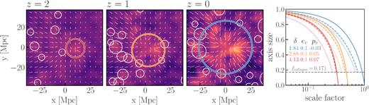
Left three panels: evolution of haloes in a 70 comoving Mpc region at three redshifts, where circles represent the radius of the Lagrangian haloes determined by the mPP method, and the background image shows the linear density field scaled by the linear growth factor. The growth and merging of haloes is immediately apparent as the central halo (coloured) grows from a mass of |$1.7 \times 10^{12}\, \mathrm{M}_\odot$| at |$z$| = 2, to a mass of |$2.6 \times 10^{15}\, \mathrm{M}_\odot$| at |$z$| = 0. White arrows show the Lagrangian displacement field, scaled down by a factor of 5, in the reference frame of the central halo at each redshift. Arrows are bent as a result of plotting the 1LPT (arrow tail) and 2LPT (arrow head) components of the displacement separately. Right-hand panel: evolution of the homogeneous ellipsoid axes (comoving size) for the most massive halo at each redshift shown on the left. Dotted, dashed, and solid lines show the collapse along the third, second, and first axes of the ellipsoid, respectively, while the colours (matched with the three left-hand panels) indicate the redshift. The third and second axes are stopped at a radial freezeout factor of |$\Delta _\mathrm{ h}^{-1/3} = 0.171$|, and the complete collapse of the first axis marks the formation redshift of the halo. Included are the values of the halo’s mean density |$\overline{\delta }$|, ellipticity eν, and prolaticity pν, which completely determine its collapse as per equation (7).
There remains freedom for the initial search radius |$R_{\mathrm{ p}_1}(R_\mathrm{ f})$|, where Rf is the filter scale that the density peak was found at, and freedom for the choices of the three radial freezeout factors, fcoll, 3, fcoll, 2, and fcoll, 1. The initial search radius is a parameter that can help to minimize underprediction of halo sizes while maximizing computational efficiency. In theory, to ensure the largest haloes are always found, one would choose |$R_{\mathrm{ p}_1}$| to be the size of the largest halo expected to be found in the entire simulation, |$R_{\mathrm{ p}_1} = R_{\mathrm{ h,max}}$|, and then step down to increasingly smaller radii until the first radius at which a halo collapses. But, this can be very inefficient, as the cost of calculating the mean strain used in the collapse equations scales as R3 (for a 0.5 Mpc resolution simulation one would then be summing over ∼1 × 10⁶ cells for every halo). Conversely, if |$R_{\mathrm{ p}_1} \simeq R_\mathrm{ f}$|, while stepping out to larger radii, a larger halo (for example of size 1.3Rf) would not be identified even though it would collapse, if a smaller halo (for example 1.2Rf) does not collapse, as the calculation is stopped when the halo centred at that location no longer collapses. We found that choosing |$R_{\mathrm{ p}_1} = 1.75 R_\mathrm{ f}$| results in a nearly identical halo catalogue to that of the theoretical best choice of |$R_{\mathrm{ p}_1} = R_{\mathrm{ h,max}}$|, at a fraction of the computational cost. This choice was adopted as the default for all future simulations.
The radial freezeout factors fcoll, i are fundamental for the homogeneous ellipsoid approximation to gravitational collapse. Two physically motivated values are |$f_{\rm {coll},i} = \Delta _\mathrm{ h}^{-1/3}$|, which corresponds to the standard top-hat virial density contrast of Δh, and fcoll, i ∼ 0, which corresponds to complete collapse along the axis. For this work, we have adopted the halo definition of |$\Delta _\mathrm{ h} = 200\overline{\rho }_\mathrm{ m}$|, where |$\overline{\rho }_\mathrm{ m}$| is the mean density of the universe. Therefore, we have the choice of fcoll, i = 200−1/3 = 0.171, or fcoll, i ∼ 0.
2.1.3 Exclusion
The final choice in the mPP method is how to ensure that collapsed regions are distinct and that there is no double counting of matter. After the computation of the homogeneous ellipsoid collapse, there will be candidate peak patches that overlap, and there will be smaller collapsed objects enveloped in larger collapsed patches. In order to prevent this unphysical result propagating to the final halo catalogue, we must perform a hierarchical Lagrangian exclusion and reduction algorithm.
![Overlapping haloes in Lagrangian space are dealt with through exclusion and reduction. Considering the binary merge [type (ii)] used for the N-body comparisons of Section 3, patch 3 would be removed from the list of candidate haloes, and both patches 1 and 2 will see a reduction in volume (mass) of V1 = V1 − V1, 2 and V2 = V2 − V2, 1, respectively. Although the volume reduction occurs only as a consequence of the spherical caps of the union of the two spheres, we treat it as a reduction of halo radius which retains the sphericity of the halo.](https://oup.silverchair-cdn.com/oup/backfile/Content_public/Journal/mnras/483/2/10.1093_mnras_sty3226/1/m_sty3226fig4.jpeg?Expires=1749913713&Signature=fkDS5YryUDoezDtCnU6QAb9NcZdFura9KIG64hRqSxA2Ow8~x9vm-cIZIHrWleSl~lKvpjkoJCep2V~IVOrkMndfxB3LIkvC3sopX8rA0knD6gTK5TQBNy9fuJP04qlkC1xQNiy0KCTK2bS717Y8caCKSzqQK19kAx5Qa5v7CqWWjbZgvgZ8F-zcK0w9BOwSB6YbduXAcZTCiQGVkGuGcKk395GP~UCuzzPikkl0hHVucKIgXL-TDjf7Po~ZJSq9fbFZ5Adhd6lIlXGRmiuUc~5xxjBP8NGuDCi~xRetuE9yoak34BKw5M~vN1T3fUiiWzLTs9MJRM5VAL8fEScnoA__&Key-Pair-Id=APKAIE5G5CRDK6RD3PGA)
Overlapping haloes in Lagrangian space are dealt with through exclusion and reduction. Considering the binary merge [type (ii)] used for the N-body comparisons of Section 3, patch 3 would be removed from the list of candidate haloes, and both patches 1 and 2 will see a reduction in volume (mass) of V1 = V1 − V1, 2 and V2 = V2 − V2, 1, respectively. Although the volume reduction occurs only as a consequence of the spherical caps of the union of the two spheres, we treat it as a reduction of halo radius which retains the sphericity of the halo.
Considering the configuration shown in Fig. 4, we have a patch p3 that will be excluded, and two overlapping spheres p1 and p2, where the volumes of overlap are V1, 2 and V2, 1. There are then three options of how to partition this overlapping mass:
Subtract the total mass (V1, 2 + V2, 1) from the larger patch.
Consider the plane perpendicular to the vector dij which divides the two spherical caps. Subtract any volume beyond this plane from each halo, V1 = V1 − V1, 2, V2 = V2 − V2, 1.
Subtract the total mass (V1, 2 + V2, 1) from the smaller patch.
The overlapping mass from all neighbouring haloes is accounted for before reducing the volumes. Although the mass reduction occurs only on the overlap between peaks, we treat it as a reduction in radius which retains the sphericity of the patch. These reductions conserve mass, but as the patches are approximated as spheres, there may still be a small overlap in volume after, which we ignore. The final radius of a halo is easily related to the mass through |$M_{\rm h} = 4\pi R_{\rm h}^3\overline{\rho }_{\mathrm{ M}}/3$|, where |$\rm {\bar{\rho }_M = 2.775 \times 10^{11} \Omega _M h^2\ [\, \mathrm{M}_\odot /Mpc^3]}$|.
The effects of binary exclusion, compared with half exclusion, were studied through a series of simulations at varying redshifts and resolutions. As expected we found that half exclusion has more haloes at all masses, as a result of not conserving mass of overlapping volumes. We find that just as in the original implementation of the mPP method, binary exclusion of type (ii) is currently the best choice. There remains the possibility to design and implement a more physical method to perform exclusion, but this is left for future work.
We note that although there most likely exists an optimal combination of choices for the filter bank, axis-freezeout, and exclusion, that might maximize a specific summary statistic when compared to a specific N-body, we do not attempt to do this. Overall, we found that the BM choices have stood well against the test of time. The parameter choices we described in this section can be seen in Table 1.
3 MASS-PEAK PATCH N-BODY VALIDATION
In this section, we validate the mPP method against N-body simulations through a number of summary statistics. By matching the initial conditions of an mPP simulation to those of the N-body run, we are able to compare halo mass functions, halo power spectra and cross-correlations, and higher order spatial matching.
3.1 Reference simulations
To test the accuracy of the mPP method, we created a suite of N-body simulations using the publicly available gadget-23 code. (Springel 2005). We ran a set of 5123 particle simulations with box sizes equal to 256, 512, and 1024 Mpc. Throughout this paper, we refer to these three sets of simulations by the comoving resolution of the 3D grid of the initial conditions: the 0.5 Mpc resolution simulation, the 1 Mpc resolution simulation, and the 2 Mpc resolution simulation. For each resolution, we ran three independent realizations, which we refer to as different simulation seeds, resulting in a suite of nine simulations in total. The following cosmological parameters were used, which match those of the Euclid comparison project: ΩM = 0.285, Ωb = 0.044, |$\Omega _\Lambda = 0.715$|, h = 0.695, ns = 0.9636, and σ8 = 0.828.
The initial conditions were generated with the publicly available 2lptic code4 using a starting time of a = 0.02 (|$z$| = 49) and a linear power spectrum generated with camb.5 The comoving force softening length (ε = 20 h−1kpc), absolute force error tolerance (α = 0.002), and time-stepping (Δ ln(a)max = 0.0125) chosen was informed by the convergence tests of the Aemulus project (DeRose et al. 2018). If we were instead targeting validations at high-redshift regime, the starting redshift would be increased to |$z$| ∼ 100.
To perform halo finding, we used the Adaptive Mesh Investigations of Galaxy Assembly halo finder, also known as AHF6 (Knollmann & Knebe 2009). We defined dark matter haloes as Eulerian-space spherical overdensities – which are themselves mPPs – of 200 times the background matter density. We use ‘strict’ spherical overdensity masses, where strict refers to the inclusion of unbound particles residing within a halo. This choice was made since we are mainly interested in the total mass of the halo and not its internal properties for this study.
For our mPP runs, we modified 2lptic to output the density and displacement fields, linearly evolved to redshift 0, instead of the 2LPT displaced particles. Each mPP simulation used the internal parameters specified in Table 1.
To create the reference Lagrangian N-body halo catalogues, we traced back each N-body halo’s constituent particles to their initial positions and calculated their centre of mass, which we define as the halo’s Lagrangian position. A halo’s Lagrangian radius is then simply |$\rm {R_{h} = (3M_{h}/4\pi \overline{\rho }_{M}))^{1/3}}$|.
A list of all runs used in this paper and their computational requirements are shown in Table 2.
A list of all validation runs included in this paper. The compute time to generate the initial conditions is not included in the timing, as this was done externally, but the timing does include reading the initial conditions from disk. Note that although the speed-up factor of these small 5123 validation runs is generally greater than a factor of 103, this factor becomes increasingly large for more massive runs, due to the straightforward parallelization of the mPP method described in Appendix A. We found a speed up factor of >3000 when comparing to the 40963 particle gadget-2 Mice Grand Challenge (Fosalba et al. 2015b; Carretero et al. 2015; Fosalba et al. 2015a), the results of which will be presented in a future work.
| Method | Nruns | Ncells | Lbox (Mpc) | Redshift | Nprocessors | Total runtime (s/run) | Memory (Gb) |
|---|---|---|---|---|---|---|---|
| Peak Patch | 56 | 10243 | 1024 | 0,1,2 | 32 | 185 | 35 |
| N-Body | 3 | 5123 | 1024 | 0,1,2 | 200 | ∼168 000 | 61 |
| Peak Patch | 3 | 5123 | 1024 | 0,1,2 | 8 | 100 | 15 |
| N-Body | 3 | 5123 | 512 | 0,1,2 | 200 | ∼168 000 | 61 |
| Peak Patch | 3 | 5123 | 512 | 0,1,2 | 8 | 140 | 15 |
| N-Body | 3 | 5123 | 256 | 0,1,2 | 200 | ∼168 000 | 61 |
| Peak Patch | 3 | 5123 | 256 | 0,1,2 | 8 | 300 | 15 |
3.1.1 Halo clustering benchmarks
As in Bond & Myers (1996a), one of the most compelling ways to compare the mPP method to N-body is by direct visual comparison of the positions of the haloes in the two catalogues, since this involves high-order clustering as well as the traditional low-order two-point correlations. To make that more precise mathematically, we introduce a new high-order statistic, by removing the mPP haloes residing inside of N-body haloes, and vice versa, using our exclusion/merger post-processing. We entitle this a halo spatial matching comparison, and present the results in Section 3.3.
We also use more traditional two-point statistics in Section 3.4 to show the power spectra of the catalogues are quite similar. We quantify this by a near-unity halo transfer function T(k), and by a more demanding halo cross-correlation coefficient, r(k), which probes the mismatch of halo centres in the two catalogues. Ideally this would have a halo-mass-dependent scaling to avoid small and large object offsets being treated exactly the same. We have not done this scaling here, since, in many respects, the first test of merging of one catalogue relative through exclusion is the more demanding scaling test.
3.2 Halo visuals
Fig. 5 provides a first, qualitative comparison of mPP haloes with those of an N-body simulation in both Lagrangian and Eulerian space. The large panels on top show a 20 comoving Mpc thick slice of the full 1024 Mpc simulation at |$z$| = 0 in Lagrangian space (left) and Eulerian space (right), while the zoom-ins on the bottom show a 200 Mpc region at |$z$| = [2, 1, 0] centred near the largest halo in the simulation at |$z$| = 0. Black circles represent the Lagrangian or Eulerian radius of the N-body haloes, while red represent mPP. The Eulerian radii were increased by a factor of 3 for visualization purposes. We see that haloes generally have the same positions and size (mass) in both methods across all redshifts, and that the large-scale structure is very well reproduced. In Lagrangian space, we also show the positions of all N-body particles which end up in haloes as the diffuse black background. We see that even N-body haloes with an aspherical Lagrangian shape are generally well matched by the mPP haloes. Shown are all N-body haloes with a mass greater than 100 cells of the simulation, ∼3 × 10¹³M⊙, and the equivalent number of mPP haloes, with no mass corrections.
![Lagrangian (left) and Eulerian (right) haloes of a 1024 Mpc simulation for both N-body (black, solid lines) and mPP (red, dashed lines). The top panels show the full simulation volume at $z$ = 0, while the bottom show a 200 Mpc zoom-in at $z$ = [2, 1, 0] centred near the largest halo at $z$ = 0. Lagrangian N-body halo positions were created by finding all particles belonging to each Eulerian halo, tracing the particles back to their initial positions (depicted here by the diffuse black background), and calculating their centre of mass. Visualized here is a 20 Mpc thick slice in the $z$-direction. The radius of the Lagrangian haloes is proportional to their mass by $R_\mathrm{ h} = (\frac{3}{4\pi \overline{\rho }_\mathrm{ M}}M)^{1/3}$, while the Eulerian radius is a factor of three larger than R200, M for visualization purposes.](https://oup.silverchair-cdn.com/oup/backfile/Content_public/Journal/mnras/483/2/10.1093_mnras_sty3226/1/m_sty3226fig5.jpeg?Expires=1749913713&Signature=lWtWbjINyZML7rEgrMlEVVoUVWogy0O8n9btK8xoPgMwNG2FYLSdjRsXxm0HxIthBAFXnEM~AE0CVHIAE6-PTmD748ROWiGr-JZZpIK3MemtXfCIpWLFHzeXJhUJ2vRw3Wq1DN6v5DljHBxj7MyB95YZjBqNcHSB76A5qSUcPRbUq6QXDfK5s6-wizfQ9OnCp9tDa6gj5ydwdK~HYMOR8XIo8ba12E3WOTsQ3ZMLgOcya02cXaAOv2zutxy2gwM-Kd-wDJWMldxizEDcnkHYJiZMX619v0eUtsrqLNsJcyC3zXQTlPC5LcdXV-ZnhFIN1~mnyNjFG8xxYHeodvaPeg__&Key-Pair-Id=APKAIE5G5CRDK6RD3PGA)
Lagrangian (left) and Eulerian (right) haloes of a 1024 Mpc simulation for both N-body (black, solid lines) and mPP (red, dashed lines). The top panels show the full simulation volume at |$z$| = 0, while the bottom show a 200 Mpc zoom-in at |$z$| = [2, 1, 0] centred near the largest halo at |$z$| = 0. Lagrangian N-body halo positions were created by finding all particles belonging to each Eulerian halo, tracing the particles back to their initial positions (depicted here by the diffuse black background), and calculating their centre of mass. Visualized here is a 20 Mpc thick slice in the |$z$|-direction. The radius of the Lagrangian haloes is proportional to their mass by |$R_\mathrm{ h} = (\frac{3}{4\pi \overline{\rho }_\mathrm{ M}}M)^{1/3}$|, while the Eulerian radius is a factor of three larger than R200, M for visualization purposes.
The relatively thin slicing of 20 Mpc in the |$z$|-direction causes some matching halo pairs to have one member in and one member out of the slice, which artificially increases the number of unmatched haloes in the visualization. As well, haloes slightly above the minimum mass boundary can have a partner of slightly lower mass, which also increases the visual discrepancy. Therefore, in the following sections, we quantify the accuracy of the mPP method in Lagrangian and Eulerian spaces with a number of halo summary statistics: halo matching, halo clustering, and the halo mass function.
3.3 Halo matching
To quantify the small discrepancies seen between the methods in Fig. 5, many of which can simply be a result of the visualization method as described in Section 3.2, we performed a quantitative analysis of the halo spatial matching between the two methods in Lagrangian space as a function of the mass of a halo. We defined an mPP halo to have an N-body partner if its Lagrangian centre of mass is within the Lagrangian radius of an N-body halo; meaning that the two haloes are constructed from roughly the same particles of the simulation. This allows for each mPP halo to classified as partnered or unpartnered. This test is a very efficient post-processing, just involving one more run of the exclusion merger program on the combined catalogues.
Fig. 6 shows a visualization of the haloes with and without partners (top), and the halo partner percentage as a function of the mass of an mPP halo (bottom). The top panel shows the same 20 Mpc thick simulation slice at |$z$| = 0 as Fig. 5, where we now instead show mPP haloes as two different colours: partnered (red) and unpartnered (grey). We see that a significant fraction of the haloes directly correspond to those of the N-body simulation. It is also clear that the only non-partnered haloes are those near the low-mass end of the simulation, and that every massive halo seen has a partner.
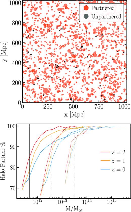
Top: partnered (red) and unpartnered (grey) Lagrangian mPP haloes in a 20 Mpc thick simulation slice at z = 0. Bottom: percentage of mPP haloes with a Lagrangian N-body partner as a function of halo mass at |$z$| = 0 (blue), |$z$| = 1 (yellow), and |$z$| = 2 (red). The linestyle indicates the resolution of the simulation, where solid, dashed, and dotted denote a 0.5, 1, and 2 Mpc resolution, respectively. Shown is the mean of the three simulation seeds. The vertical lines denote the mass of 100 particles for each simulation resolution.
The bottom panel shows the halo partner percentage as a function of mass for the three simulation resolutions and three redshifts. For large halo masses, the partner ratio is very close to unity for all simulation resolutions and redshifts, as expected from the top panel. The linestyle indicates the resolution of the simulation, while the colour shows the redshift of the halo catalogue. Solid, dashed, and dotted lines denote a 0.5, 1, and 2 Mpc resolution, while red, yellow, and blue denote redshifts of |$z$| = 2, 1, and 0, respectively. As the halo mass decreases to the mass of 100 particles of the simulation (vertical black lines), which is the smallest halo we expect to accurately resolve, the partner ratio decreases to 90 per cent for the 2 Mpc resolution simulation for all redshifts, while for the 1 Mpc (0.5 Mpc) resolution simulations, we see a variation as a function of redshift from |${\sim } 90 {{\ \rm per\ cent}}$| at |$z$| = 2 to |${\sim } 80 {{\ \rm per\ cent}}$| at |$z$| = 0 (|${\sim } 80 {{\ \rm per\ cent}}$| at |$z$| = 2 to |${\sim } 70 {{\ \rm per\ cent}}$| at |$z$| = 0) for a 100 particle mass halo. For all simulation resolutions and redshifts, we find a high partnerpercentage of |$\ge 90{{\ \rm per\ cent}}$| for haloes above a mass of ∼200 particles in the simulation.
3.4 Halo clustering
The two- and three-point clustering of haloes above various mass cuts in simulations are commonly used quantifications of the accuracy of approximate methods when compared to full N-body simulations. Recently, mPP clustering results were presented in a series of three papers (Lippich et al. 2019; Blot et al. 2018; Colavincenzo et al. 2018) which investigated the accuracy of six different approximate methods [HALOGEN (Avila et al. 2015), ICE-COLA (Izard et al. 2016), lognormal (Agrawal et al. 2017), mass-Peak Patches, PATCHY (Avila et al. 2015), and PINOCCHIO (Monaco et al. 2013)] when compared to N-body for the purpose of creating mock catalogues and covariance matrices for the Euclid collaboration. Also included was the Gaussian recipe of Grieb et al. (2016) which created covariance matrices only. All methods but the lognormal one simulated 300 independent realizations with matching initial conditions of a 10003 dark matter particle box, with a side length of 2158 Mpc, to create 300 halo catalogues at |$z$| = 1.
Lippich et al. (2019) investigated the correlation function results, Blot et al. (2018) investigated the power spectrum results, and Colavincenzo et al. (2018) performed a comparison of the halo bispectrums. When considering abundance matched haloes above a minimum mass cut of 100 particles (the only mass sample we provided because of our concerns about patches defined on small numbers of lattice sites), mPP fared well across all halo summary statistics, remaining consistently among the top few methods. Along with ICE-COLA, it performed best on the mean and the variance of the power spectrum multipoles, and alongside ICE-COLA and PINOCCHIO, it performed best on the mean and the variance of the bispectrum. One interesting result of the bispectrum analysis was that the difference between predictive and abriged particle mesh methods compared to stochastic methods became much greater than for the power spectrum or correlation function, with the exception of PATCHY which fared well. This can partially be attributed to the fact that stochastic methods work by tuning parameters until they can best match specific summary statistics of a few of the N-body runs, such as the correlation function. When then asked to create a halo catalogue to encapsulate a clustering statistic that the method was not fit to (such as capturing the correct bispectrum when the parameters of method were fit to give an accurate correlation function), they tend to greatly decrease in accuracy.
This comparison project was very broad in scope, but it was limited to a single simulation resolution of ∼2 Mpc, and a single redshift of |$z$| = 1. In this work, we expand upon this by looking at three different simulation resolutions and three different redshifts. Although the mPP method is a Lagrangian space halo finder, the final Eulerian state accuracy is generally more important for the desired use of creating large-volume mock halo catalogues to model cosmological observables and their covariances. In the mPP method, haloes are moved to their Eulerian positions by calculating the average Lagrangian displacement of every particle belonging to a halo, and for this study, the displacements are calculated using second-order LPT. Going to an even higher order LPT (at a cost of computational efficiency and memory) has been shown to slightly improve halo displacements in the PINOCCHIO method when compared to N-body (Munari et al. 2017). Because of the halo-adaptive smoothing inherent in mPP, it is unclear that higher order LPT will be of use, but we leave this for further study: a modest boost in accuracy may not be worth the trade-off in efficiency.
3.4.1 Lagrangian halo clustering
Fig. 7 shows the halo clustering results in Lagrangian space as a function of redshift for the three simulation resolutions. The top row shows the transfer function of the Lagrangian particles that belong to haloes, the middle row shows the transfer function of the Lagrangian halo positions, and the bottom row shows the cross-correlation coefficient of the Lagrangian particles that belong to haloes. Each line is the mean of the three simulation seeds. The colour indicates the redshift of the analysis, where blue, yellow, and red represent |$z$| = 0, 1, and 2, respectively, and the linestyle indicates the minimum number of particles per halo, where dotted, dashed, and solid show a 50, 100, and 500 particle minimum. The conversion from number of particles to halo mass is simply |$M_{\rm {min}} = 3.82{\times }10^{12} (\frac{\rm {resolution}}{1\rm \,{Mpc}})^3 (\frac{\rm {N_{particle}}}{100}) \, \mathrm{M}_\odot$|. The lines not shown at |$z$| = 2 are due to the insufficient number of haloes found in both methods to perform a meaningful power spectrum calculation.
![Lagrangian space. Top row: transfer function of the Lagrangian particles that belong to haloes. Middle row: transfer function of the Lagrangian halo positions. Bottom row: cross-correlation coefficients of Lagrangian particles that belong to haloes. The Lagrangian radius of the largest halo expected at $z$ = [0, 1, 2] is roughly Rh = [30 Mpc, 15 Mpc, 10 Mpc]. Translating this to a wavenumber results in k ∼ [0.1 Mpc−1, 0.15 Mpc−1, 0.2 Mpc−1], which is nearly exactly where we see the deviation of the mPP Lagrangian particle transfer function and particle cross-correlation function from the N-body. This is expected, as mPP haloes are strictly spherical, while the N-body are not. Additionally, we have not abundance matched the haloes in mass, meaning that the total number of particles in mPP haloes is not equivalent to N-body in this comparison. Each panel shows the mean results of the three simulation seeds at $z$ = 0 (blue), $z$ = 1 (yellow), and $z$ = 2 (red), for three halo particle number cuts. The linestyle indicates the minimum number of particles per halo, where dotted, dashed, and solid show a 50, 100, and 500 particle minimum, respectively. The conversion from number of particles to halo mass is simply $M_{\rm {min}} = 3.82{\times }10^{12} (\frac{\rm {resolution}}{1\rm \,{Mpc}} )^3 (\frac{\rm {N_{particle}}}{100}) \, \mathrm{M}_\odot$.](https://oup.silverchair-cdn.com/oup/backfile/Content_public/Journal/mnras/483/2/10.1093_mnras_sty3226/1/m_sty3226fig7.jpeg?Expires=1749913713&Signature=ELelF0txnPf7s82ExEuteaQNU~8l9jdEvLzx5xa-91ZB9JxX2SizgElAx2u-nq-5CTPLbwFUcu81ApooKCalRQJ35HXRRrtWIBsat9XOrNjiSYwvPNhGq4dogFN5b~RRgFr9IXIUHPfcHrEmHrxUJrhqx7pw65CjatHa9nSMXZ1hHlbD6LHZFrd0-DO-b8BwKR~8IY3xkT~52nu1aQaMwJN-zmecnSd2YQDMVEg1CByT48RjBVoPWCgQzeiOIAUSwQ8bKF00yTAJBEGX5cKOQoba30OzYcyCtaGqduxYVTnrXCozecnMfFuD1fGLwaXm5xfj13z7lVUoDk0N7Jzwdw__&Key-Pair-Id=APKAIE5G5CRDK6RD3PGA)
Lagrangian space. Top row: transfer function of the Lagrangian particles that belong to haloes. Middle row: transfer function of the Lagrangian halo positions. Bottom row: cross-correlation coefficients of Lagrangian particles that belong to haloes. The Lagrangian radius of the largest halo expected at |$z$| = [0, 1, 2] is roughly Rh = [30 Mpc, 15 Mpc, 10 Mpc]. Translating this to a wavenumber results in k ∼ [0.1 Mpc−1, 0.15 Mpc−1, 0.2 Mpc−1], which is nearly exactly where we see the deviation of the mPP Lagrangian particle transfer function and particle cross-correlation function from the N-body. This is expected, as mPP haloes are strictly spherical, while the N-body are not. Additionally, we have not abundance matched the haloes in mass, meaning that the total number of particles in mPP haloes is not equivalent to N-body in this comparison. Each panel shows the mean results of the three simulation seeds at |$z$| = 0 (blue), |$z$| = 1 (yellow), and |$z$| = 2 (red), for three halo particle number cuts. The linestyle indicates the minimum number of particles per halo, where dotted, dashed, and solid show a 50, 100, and 500 particle minimum, respectively. The conversion from number of particles to halo mass is simply |$M_{\rm {min}} = 3.82{\times }10^{12} (\frac{\rm {resolution}}{1\rm \,{Mpc}} )^3 (\frac{\rm {N_{particle}}}{100}) \, \mathrm{M}_\odot$|.
For the Lagrangian-space halo particles (top), we find that the transfer function is flat on large scales (small k), and within |$5-10{{\ \rm per\ cent}}$| for all simulation redshifts, number cuts, and resolutions. On small scales (large k), we find that mPP has more power. This is expected since mPP haloes are taken to be strictly spherical in Lagrangian space, while N-body haloes are strictly spherical in Eulerian space, hence not when mapped back to in Lagrangian space. The Lagrangian radius of the largest halo expected at |$z$| = [0, 1, 2] is roughly Rh = [30 Mpc, 15 Mpc, 10 Mpc]. Translating this to a wavenumber results in k ∼ [0.1 Mpc−1, 0.15 Mpc−1, 0.2 Mpc−1], which is nearly exactly where we see the deviation of the mPP Lagrangian particle transfer function from the N-body. Additionally, we have not abundance-matched the haloes in mass, hence the total number of particles in mPP haloes is not equal to those in the N-body haloes.
The transfer function for the Lagrangian halo positions (middle) is flat on all scales for the 1 and 2 Mpc resolution simulations, though with some scale dependence on large scales for the 0.5 Mpc resolution simulation, similar to what is seen in the Eulerian case. For both the 1 and 2 Mpc simulation resolutions, the transfer function is within |$5{{\ \rm per\ cent}}$| for |$z$| = 1 and 2, and within |${\sim }7{{\ \rm per\ cent}}$| for |$z$| = 0. For the 0.5 Mpc resolution simulations, we see more deviation at the large scales. When considering k > 0.1 Mpc−1, we see that for all simulation redshifts, number cuts, and resolutions the transfer remains within |$7{{\ \rm per\ cent}}$|, but for the 0.5 Mpc resolution simulation it deviates by up to |$25{{\ \rm per\ cent}}$| for k < 0.1 Mpc−1. This may be attributed to the small 256 Mpc size of the box: more investigation is needed.
The cross-correlation coefficient of the Lagrangian halo particles (bottom) is close to unity for all simulation redshifts and resolutions at large scales. For the 0.5 Mpc resolution simulation we find, for redshifts |$z$| = [0, 1, 2], that r ≥ 0.95 at k = [0.2 Mpc−1, 0.3 Mpc−1, 0.4 Mpc−1], and that r ≥ 0.9 at k = [0.3 Mpc−1, 0.45 Mpc−1, 0.6 Mpc−1]. For the larger resolution simulations, there is a small decrease at high k values, which is to be expected as these small spatial scales are unresolved. The higher particle number cuts, or more massive haloes, have a lower cross-correlation coefficient than the low number cuts which is most pronounced at |$z$| = 0. Although this decrease appears to be counterintuitive, as we have shown throughout this work that the mPP method generally performs better for larger haloes, it can be attributed to a slight miscentring by a few lattice sites for large haloes, which is largely mitigated in the displacement to Eulerian space as we discuss further at the end of the next subsection. Large haloes with centres separated a small fraction of their overall Lagrangian size, e.g. by one or two lattice sites, will still be composed of |${\sim } 95{{\ \rm per\ cent}}$| of the same particles for two 30 Mpc haloes, but will not result in a particularly high Lagrangian cross-correlation coefficient at large values of k.
3.4.2 Eulerian halo clustering
Fig. 8 shows the halo clustering results in Eulerian space as a function of redshift for the three simulation resolutions. The top two rows show the transfer function in real space and redshift space, while the bottom two rows show the cross-correlation coefficient. Each line is the mean of the three simulation seeds. The colour indicates the redshift of the analysis, where blue, yellow, and red represent |$z$| = 0, 1, and 2, respectively, and the linestyle indicates the minimum number of particles per halo, where dotted, dashed, and solid show a 50, 100, and 500 particle minimum. The lines not shown at |$z$| = 2 are due to the insufficient number of haloes found in both methods to perform a meaningful power spectrum calculation.
![Eulerian space. Halo transfer function (top two rows) and cross-correlation coefficient (bottom two rows) of the N-body and mPP halo catalogues in Eulerian space at $z$ = [0, 1, 2], in both real space and redshift space, for three particle number cuts. Shown is the mean of the three simulation seeds. Each panel demonstrates the mean results of the three simulation seeds at $z$ = 0 (blue), $z$ = 1 (yellow), and $z$ = 2 (red), for three halo particle number cuts. The linestyle indicates the minimum number of particles per halo, where dotted, dashed, and solid indicate a 50, 100, and 500 particle minimum, respectively.](https://oup.silverchair-cdn.com/oup/backfile/Content_public/Journal/mnras/483/2/10.1093_mnras_sty3226/1/m_sty3226fig8.jpeg?Expires=1749913713&Signature=xxZcQiK9pzoUciW2MrtJuN16pGIOu7-75qafmtgrjPY1HL-FPHJQtdN1c-n1s7mFBEvhyV0zopO-7~DRxoiDnMjiCWydT6VxjUKk3htTBrcv6X5502JjEbj~HxKFb3T8HnyLtiNu34akDJELjLfLtq7Nr197aCr3JwMzGjQYOExl~TRoOZ4Fk4gr-gJhh-pVE2uqQsza68MeQfeTID14qfJrNKVfIwPLoNWLkLn7oCDS6X0vOux8NL2WxJ96dEMMBxuapz4H0Hg~NI~7EypUl3MdbpmLK~6fNUdDv35JVbnkOhEhb1-rRHoVaq~LgvOIQON6VygfsChhl8pwigNXHQ__&Key-Pair-Id=APKAIE5G5CRDK6RD3PGA)
Eulerian space. Halo transfer function (top two rows) and cross-correlation coefficient (bottom two rows) of the N-body and mPP halo catalogues in Eulerian space at |$z$| = [0, 1, 2], in both real space and redshift space, for three particle number cuts. Shown is the mean of the three simulation seeds. Each panel demonstrates the mean results of the three simulation seeds at |$z$| = 0 (blue), |$z$| = 1 (yellow), and |$z$| = 2 (red), for three halo particle number cuts. The linestyle indicates the minimum number of particles per halo, where dotted, dashed, and solid indicate a 50, 100, and 500 particle minimum, respectively.
In real space we find that the transfer function (top row) is nearly flat at large scales for all simulation resolutions, but shows a scale dependence on large scales that increases between z = 2 and 0 for the 0.5 Mpc resolution simulation. For both the 1 and 2 Mpc simulation resolutions, we find that the transfer function is within |$5{{\ \rm per\ cent}}$| for all redshifts and number cuts for the entire k range. Considering the 2 Mpc resolution simulation, at |$z$| = [0, 1, 2], the transfer function agreement is within |$[5{{\ \rm per\ cent}}, 2.5{{\ \rm per\ cent}}, 1{{\ \rm per\ cent}}]$|, and for the 1 Mpc resolution simulation, the agreement at |$z$| = [0, 1, 2] is within |$[5{{\ \rm per\ cent}}, 2.5{{\ \rm per\ cent}}, 2.5{{\ \rm per\ cent}}]$|, across the entire k range. For the 0.5 Mpc resolution simulation, the transfer function remains within |$10{{\ \rm per\ cent}}$| for all redshifts and number cuts. We also find that the cross-correlation coefficient of the halo positions (third row) remains high for all resolutions, particle number cuts, and redshifts. The transfer function results of the Euclid comparison project, Blot et al. (2018), a ∼2.2 Mpc resolution simulation at z = 1, are nearly identical in amplitude to the results shown in Fig. 8 by the dotted yellow line (z = 1) of the 2 Mpc resolution simulation, adding further validation to mPP simulations compared with N-body simulations.
In redshift space, we find nearly identical results to those in real space for the 2 and 1 Mpc simulation resolutions. For the 0.5 Mpc resolution, we find that the transfer function (second row) actually improves for |$z$| = 2 and 1, but shows much more scale dependence at |$z$| = 0, which is not unexpected as these halo velocities have contributions from more non-linear effects. The cross-correlation coefficient (bottom row) for the 0.5 Mpc resolution simulation decreases slightly when compared to the real space version, but has no qualitative differences.
We find the same exercise for Lagrangian space halo positions reveals more deviation, largely attributable to not adding a mass-dependent position uncertainty: the large haloes encompass enormous regions of Lagrangian space. After dynamical evolution, this effect is partly mitigated, but even for the Eulerian space tests a radius-scaling associated with positional uncertainty would further improve the halo–halo cross-correlation coefficients. One way to do this is to create a 3D map from the catalogue by adding a halo–radius Gaussian uncertainty. The merger test described above uses top hats rather than Gaussians, and uses the halo radius rather than a range of fuzziness scales, but has more statistical content than the power spectra of these 3D fuzzy maps so we have not pursued the fuzzy-halo approach further in this paper.
3.5 Mass function
Though the halo mass functions are well reproduced, we note that even if only roughly correct we could still have an accurate method for creating mocks of the large-scale structure of the universe. It is straightforward to abundance match the mass of haloes through a few small simulations, or through universal halo mass functions, so the main criterion for accuracy is that the mass ranking of the haloes of the approximate method matches that of the N-body, and that a sufficient number of haloes are detected (Lippich et al. 2019; Blot et al. 2018; Colavincenzo et al. 2018). The results of the number matched transfer function and cross-correlation coefficient of Fig. 8 show that this is indeed true for the mPP method.
The halo mass function of the simulations, with no abundance matching or tuning, can be seen in Fig. 9. We show the mean of the three simulation seeds, where solid, dashed, and dotted lines denote a 0.5, 1, and 2 Mpc simulation resolution, respectively, and the colours blue (|$z$| = 0), yellow (|$z$| = 1), and red (|$z$| = 2) indicate the redshift. The vertical lines show where our effective mass cut-off of 100 cells (particles) lie as the resolution varies, and the grey bar on the bottom panel shows the ±10 per cent deviation of the mPP from N-Body. We also show the conventional characterization of the mass spectrum M*, defined by σ(M*) = 1.686, and the ‘non-linear’ mass Mnon-lin defined by σ(M*) = 1.686 (σ(Mnon-lin) = 1.0, as ⋆ and |$\boldsymbol{+}$| symbols, respectively.
![Halo mass functions at $z$ = [0, 1, 2]. Shown is the mean of the three simulation seeds for each redshift and simulation resolution. Linestyle indicates the resolution of the simulation, where solid, dashed, and dotted denote a 0.5, 1, and 2 Mpc simulation resolution, respectively. The thick black lines in the upper panel, which both mPP and N-body accurately match, show the universal mass function of Tinker et al. (2008). The vertical lines illustrate the mass of 100 cells (particles) of a simulation for each simulation resolution, and the grey bar on the bottom panel denotes a ±10 per cent deviation of Peak Patch from N-Body. The ⋆ symbols show the value of M* at each redshift, while the $\boldsymbol{+}$ symbols show the value of Mnon-lin.](https://oup.silverchair-cdn.com/oup/backfile/Content_public/Journal/mnras/483/2/10.1093_mnras_sty3226/1/m_sty3226fig9.jpeg?Expires=1749913713&Signature=j0q3-3cmNwcRhoCPLEkoJTbiGrecaCHMrzruoYyQKoOlLTOemTCOERUyjatlL01cPUUWurYK~v-dIJCkyp54HigZeHXECsRPXXHfD~NCgzT7SNBHT3VGHjqGG56oFFiPuzDHx~QH5bjbnMuRzXttYz~Gy9dfGGFe0LsqC1MxfbDGA7GPUohVRlOJmTGx07XoCZYLBD~cOBpj6ib5pnKYy5yx3hVqmQwmZr0fV81fouI-ZS1bWTDRD6UM~5hsvTDBQvFnzAdZ9WUXWchD536KrnKLTdk4uA1L-wL066ElXoGEVazmTwq6oCjTfrBHJWIv0Bz0Ed9q95G7mWhpoXPBOg__&Key-Pair-Id=APKAIE5G5CRDK6RD3PGA)
Halo mass functions at |$z$| = [0, 1, 2]. Shown is the mean of the three simulation seeds for each redshift and simulation resolution. Linestyle indicates the resolution of the simulation, where solid, dashed, and dotted denote a 0.5, 1, and 2 Mpc simulation resolution, respectively. The thick black lines in the upper panel, which both mPP and N-body accurately match, show the universal mass function of Tinker et al. (2008). The vertical lines illustrate the mass of 100 cells (particles) of a simulation for each simulation resolution, and the grey bar on the bottom panel denotes a ±10 per cent deviation of Peak Patch from N-Body. The ⋆ symbols show the value of M* at each redshift, while the |$\boldsymbol{+}$| symbols show the value of Mnon-lin.
We find that the homogeneous ellipsoidal collapse approximation and binary exclusion of the mPP method produces a halo mass function that agrees with the results from N-body, generally to |$10{{\ \rm per\ cent}}$| for all simulation resolutions and redshifts above a minimum halo mass cut of 100 particles. At the highest mass end, we see a slightly larger deviation, but this can be attributed to the small number statistics of haloes in the largest bins. We also find that mPP reproduces the mass function within |$\pm 10{{\ \rm per\ cent}}$|, even to below the non-linear scale Mnon-lin, at all redshifts and simulation resolutions. As in BM, we prefer the spherical overdensity approach to Eulerian halo finding as one more closely matched to what is done in the mPP algorithm, rather than, e.g. the often used friends-of-friends method. More dynamically refined advanced halo finding based on detailed orbits is not really suitable for comparison with mPP haloes.
3.6 Additional validations
Our results on validation are robust across a broad range of simulation resolutions and cosmological parameter choices. Grid cell masses of 2.5 × 10|$^{8}$| up to 2.6 × 10|$^{11}\, \mathrm{M}_\odot$| have been used in various simulations, without any significant change to the accuracy of the mass function or power spectrum when compared to a universal halo mass function or an N-body simulation of the same resolution. Flat ΛCDM cosmologies with ΩM = (0.2–0.35), ns = (0.75–0.9), and σ8 = (0.7–0.9), have also had no qualitative or quantitative effect on the accuracy of the method when compared to N-body.
We briefly now report on other tests we have done over the years in the lead-up to the current analysis. We compared mPP to spherical overdensity halo catalogues constructed from a suite of simulations created with the cubep3mN-body code (Harnois-Déraps et al. 2013), that covered the cluster formation and galaxy formation range of redshifts shown here, but, more importantly, were extended to cover the early galaxy regime at higher redshifts, where the power spectrum has almost equal power per decade, presenting challenges because of the large cross-talk among quite disparate wavenumbers. A set of mPP and cubep3m simulations with box sizes of 857, 215, and 6.43 Mpc (at |$z$| = 10.6) were constructed from matching initial conditions. These showed halo biasing factors were accurately reproduced. At that time adaptive 1LPT was used to move the haloes rather than our now standard 2LPT. Even so, the 6.43 Mpc simulations showed the mPP method was able to reproduce the remarkably deformed spatial structure of large voids at |$z$| = 10.6, in spite of the challenges of nearly flat density power and extremely large-scale tides. Although in the work presented here we have focused on using simulations at lower redshifts to further our validation, we are confident the mPP method can accurately simulate halo catalogues at high redshifts: the ‘first star’ regime and the epoch of reionization.
4 DISCUSSION AND CONCLUSIONS
In this work, we presented an updated and massively parallel version of the mPP method of Bond & Myers (1996a), an accelerated method for generating simulations of the large-scale structure of the universe. Motivated by the requirements of future large-scale structure and CMB surveys and their need for ensembles of large-volume mocks, we have shown that this method (described in Section 2), designed to run on massively parallel computing architectures, produces accurate dark matter halo catalogues over 3 orders of magnitude faster than N-body, at a fraction of the memory cost. In Appendix A, we discuss the performance and parallelization of the method in detail.
The mPP method explicitly models nonlinear halo collapse and exclusion. As such, it does not require calibration with respect to N-body simulations, since the basic ingredients of coarse-grained local ellipsoidal dynamics into the non-linear regime, hierarchical exclusion of small-scale entities within larger scale entities, and bulk motion and flow, are invariant. Radically varying cosmological parameters does not alter the algorithm, nor does focusing on different halo definitions. This allows modular improvements to be straightforwardly incorporated, e.g. improving flow dynamics beyond 2LPT, adding non-CDM forces to ellipsoidal dynamics, or extending to all manner of beyond the standard model of cosmology situations. Thisdoes not mean that there are not fun challenges, e.g. incorporating scale-dependent dark matter components into the ellipsoid collapse model.
In Section 3, we compared the accuracy of the method to that of N-body simulations across a broad range of redshifts, |$z$| = [0, 1, 2], and simulation resolutions, [0.5 Mpc, 1 Mpc, 2 Mpc]. We presented a variety of halo summary statistics and showed that, without any parameter tuning, the algorithm produces accurate results. The higher order spatial matching of the mPP halo catalogues was investigated in Section 3.3, the Eulerian and Lagrangian clustering was presented in Section 3.4, and the halo mass function results were shown in Section 3.5. This follows on from the vintage Bond and Myers validations of the nineties, and sporadic, but instructive, validation exercises subsequently. The most important of those not presented here, in our regard, is the demonstration that the mPP algorithm can successfully treat the tidally extreme regime from which the first small objects emerge at high redshift when compared to cubep3mN-body simulations.
The accuracy of the halo summary statistics presented in this work make the mPP method well suited for creating large ensembles of dark matter halo catalogues to mock current and next-generation cosmological surveys, ensembles to aid in complex statistical interpretations of the standard model of cosmology and likelihood function creation, and ensembles with cosmic parameters extended to describe beyond the standard model of cosmology. In a forthcoming paper (Alvarez et al., in preparation), we describe the set of publicly available full-sky extragalactic simulations that we have developed for current and future CMB surveys.7
ACKNOWLEDGEMENTS
We thank J.D. Emberson for providing cubep3m halo catalogues, and Philippe Berger for helpful discussions.
Research in Canada is supported by NSERC and CIFAR. These calculations were performed on the GPC and Niagara supercomputers at the SciNet HPC Consortium. SciNet is funded by: the Canada Foundation for Innovation under the auspices of Compute Canada; the Government of Ontario; Ontario Research Fund – Research Excellence; and the University of Toronto.
Footnotes
This differs from a common definition of ‘predictive’ used in the field, where a predictive method is instead defined as any method that ‘finds’ haloes in a given density field – initial or final. Using this definition instead would then also include N-Body, COLA, FastPM, and, arguably, the second implementation of PThaloes.
REFERENCES
APPENDIX A: PARALLELIZATION AND PERFORMANCE
A1 Performance
Fig. A1 shows the weak-scaling performance of the mPP method. Although we have easily run mPP simulations of a grid size of 61443 cells, these were unable to be included in the figure due to the set-up of the compute cluster used for these tests, which prevented us from keeping the same ratio of processors to simulation volume due to a lack of memory per node. For reference, when comparing to the 40963 particle Mice Grand Challenge simulation which required |${\sim }3\, 100\, 000$| CPU hours (Carretero et al. 2015; Fosalba et al. 2015a,b), mPP required a total compute time of ∼1000 h, a speed up factor of over 3000. The weak-scaling test shows that as the simulation size increases, the generation of the initial conditions starts to become the dominating factor, showing the computational efficiency of the Peak Patch algorithm.

Weak-scaling relation of the mPP method on Intel Xeon EE540 2.53 GHz CPU cores of the Scinet-GPC cluster. A fixed lattice resolution of 2 Mpc was chosen, while the number of cells and number of processors was increased accordingly. Each processor computes ∼2803 cells representing a volume of ∼5123 Mpc. The black solid line shows the total time for the simulation. Blue lines are for setting up the initial conditions, orange are for the main halo finding and exclusion algorithims, and green are for the data output. We see that as the simulation size increases, the generation of the initial conditions starts to become the dominating factor, showing the power of the mPP method.
A2 Parallelization
The initial conditions used for running an N-body or an mPP simulation are in the form of a monolithic cubic periodic grid. As the mPP algorithm needs only semilocal information about neighbouring grid cells to determine the size and location of dark matter haloes, this total cubic volume can be divided into sub-regions with an extra buffer added, each sub-region can be passed to a different compute node or (group of) processor(s), and the full calculation can continue without any further message passing. This allows for the simulation to proceed much more rapidly than N-body calculations which require the entire volume to be evolved at the same time, which necessitates complicated message passing.
Fig. A2 shows the domain decomposition of the updated mpi implementation of the mPP algorithm. We create the 3D initial conditions using a 1D (or ‘slab’) decomposition, and perform Fast Fourier Transforms using the FFTW3 library.8 A slab decomposition has the limitation that, given a cubic simulation of size N3, only N processors can be used to calculate the initial conditions, as each mpi process has to contain at least one slab of data. Although this is a problem for certain types of cosmological simulations, for mPP it is not a limiting step. Each mPP sub-region requires a buffer to allow for haloes near the edge of the sub-volume to be properly calculated (shown in Fig. A2 as the light blue shaded region when considering cube 0). This buffer is usually a non-negligible fraction of the total volume, e.g. a 2563 region which needs an additional buffer of 32 cells on a side will have a ‘usable volume fraction’ of (256/(256 + 32 × 2))3 = 0.512. If we consider the case of N processors for an N3 cubic simulation which we divide into N sub-volumes (in the case of no threading), by increasing the number of processors by a factor of 23 each sub-volume will decrease to a size of 1283, meaning the usable volume fraction drops to (128/(128 + 32 × 2))3 = 0.296, and the buffer starts to dominate the compute resources. Therefore, it is better to utilize shared memory multiprocessing through openmp9 and use more threads per process in this scenario. For this reason, we designed mPP to also use openmp for the compute heavy calculations, such as smoothing the density cubes to find density peaks and the homogeneous ellipsoid calculations, and there is no current need to implement a 2D (or ‘pencil’) decomposition.
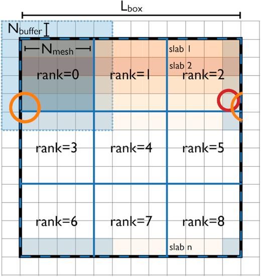
Parallelization set-up of the mPP method. The 3D initial conditions are created using a slab decomposition, where slabs (shaded in orange) are spread evenly across all mpi processes. Slabs are then re-arranged into cubes, using an additional buffer region (light blue shaded region when considering cube 0) in order to properly perform halo finding on regions near a cube boundary (examples shown by the red and orange haloes). mpi processes then independently find haloes and calculate their properties, requiring no further message passing until the calculation is complete and halo catalogues are written to disc.
The simplicity of homogeneous ellipsoid collapse and the parallelization scheme also allows for light-cone simulations to be created on the fly. This saves a large computational cost when compared toN-body or abridged particle mesh methods, which usually require finely spaced snapshots to be written to disc, halo finding to be performed, and the resulting catalogues to be stitched together. Fig. A3 shows how light-cones are created in the mPP method for no extra computational cost when compared to a single redshift simulation. The comoving distance from the observer to the halo in question is translated into a redshift, and the size of each halo is then determined by calculating the radius of the largest homogeneous ellipsoid that will collapse by that redshift. The first- and second-order halo displacement vector is scaled by the appropriate linear growth factors before moving the halo to its final Eulerian position along the light-cone.
![The simplicity of homogeneous collapse allows for light-cone simulations to be created on the fly. The comoving distance from the observer (placed here in the centre of the box) to the halo in question (h1, h2, and h3 in this example) is translated into a redshift, $z$ = [$z$1, $z$2, $z$3]. The size of each halo is then determined by calculating the radius of the largest homogeneous ellipsoid that will collapse by that redshift, and the first- and second-order halo displacement vectors are scaled by the appropriate factors of the linear growth factors before moving the halo to its final Eulerian position along the light-cone.](https://oup.silverchair-cdn.com/oup/backfile/Content_public/Journal/mnras/483/2/10.1093_mnras_sty3226/1/m_sty3226figa3.jpeg?Expires=1749913713&Signature=ZnWErKvolxB6v4XaLpasFUb~Sx7aSLmXHDsl9enFBZ0ULMFFegtnclPsmc04Uz4xVXYw6SrC8yWv9m-nsAIUXd5luNBJY3gtAAoPkIpqi4jaIROJyqb8vq0d1ImleiBbZPSgspmMd~CNGGLh6cBsDDfvXefN8z5S4jWlyVhbe8mWWEP4Xsw~tLowDN6~qGrIDmPeym~EN4hMsjPswKxBdTcu7A9yhfTUQSzV-PCNEyKFJgCtppONHH2hLLHRcuBlupqbwGg8z7IXEj2rBk4XK0Nyol2lkO~4A~~8KNvTlZB6hYb9BQc-fwnIkrpRwdBk1nUxNZgIFXE8RMcO7qgc7g__&Key-Pair-Id=APKAIE5G5CRDK6RD3PGA)
The simplicity of homogeneous collapse allows for light-cone simulations to be created on the fly. The comoving distance from the observer (placed here in the centre of the box) to the halo in question (h1, h2, and h3 in this example) is translated into a redshift, |$z$| = [|$z$|1, |$z$|2, |$z$|3]. The size of each halo is then determined by calculating the radius of the largest homogeneous ellipsoid that will collapse by that redshift, and the first- and second-order halo displacement vectors are scaled by the appropriate factors of the linear growth factors before moving the halo to its final Eulerian position along the light-cone.
