


Abstract
The spectra from Fe-peak elements may be used to determine the temperature and density of various astrophysical objects. Determination of these quantities is underpinned by the accuracy and the comprehensiveness of the underlying atomic structure and collisional calculations. In the following paper, we shall focus specifically on Ni iv lines associated with transitions amongst several low-lying levels. We shall employ modified versions of the parallel Dirac R-matrix codes, considering both electron-impact excitation of Ni3+ and the photoionization of both the ground and excited states of Ni2+. We produce high-quality data sets for both processes, and using these data, we calculate line ratios relevant for plasma diagnostics of temperature and density.
1 INTRODUCTION
The spectra of lowly ionized iron-peak elements such as (Feq+, Coq+, Niq+, q = 0−3) are vitally important in astronomical observation. In particular, Ni3+ being iso-electronic with Fe+ should produce many of the same diagnostic lines, which have extensively been studied previously by Pradhan & Berrington (1993), Zhang & Pradhan (1995), Ramsbottom et al. (2005, 2007), and Ramsbottom (2009). Comparisons of these lines using the results of the present paper shall be made. The Fe-peak elements provide some of the most abundant species created inside the stars, and they emit at ultraviolet wavelengths, making them dominant contributors to the opacity of the interstellar media under certain conditions.
From an atomic physics perspective, the half-open d-shell nature of many of these systems inevitably leads to target descriptions involving between 20 and 30 configurations if spectroscopic accuracy is to be approached. The N + 1-electron collisional calculation, whether it be excitation or photoionization expands to target descriptions involving between 5000 and 7000 levels with the associated cost of calculating over 109 Racah angular coefficients. Only with the development of the current suite of codes, including multiple layers of hyper-threaded parallelism, the Hamiltonian formation being the most critical part, have we been able to make progress on these type of systems. It has enabled us to provide comprehensive data sets that include every excitation and de-excitation for electron-impact excitation (EIE) or photoionization (PI), not just from the ground state, but as well from every excited state.
Several groups throughout the world (The Opacity Project Team 1995),1 OPAL (Iglesias & Rogers 1996),2 recognize that calculated opacities are essential for the correct interpretation of the spectra taken from a variety of objects, such as interstellar clouds, nebulae, remains of supernovae and stellar atmospheres. Even today, there are still remaining outstanding issues with experimental measurements that do not agree with any of the predicted models listed above (Bailey et al. 2014). We note that fundamental atomic data is only one aspect of the complex plasma-modelling codes, but the ability to put a realistic uncertainty on first principle calculations can eliminate it as the cause of disagreement with experimental observations. This has spurred the calculation of uncertainties with every collisional process, that are both a function of temperature and density. Our long-term goal is to ensure that the astrophysical modelling packages such as cloudy (Ferland et al. 2017),3xstar4 can integrate not only new atomic collisional data but also the associated uncertainty file.
One long-term project that recognized the need for comprehensive photoionization of every ion stage for a large part of the periodic table is the Opacity Project (The Opacity Project Team 1995). The distribution of work on various atomic species was calculated by theoretical physics groups across the world and provided a very fruitful collaboration. However, as the near-neutral species are highly complex and the former computational resources were insufficient to calculate them, the Opacity Project saw a greater focus on the more highly ionized systems. With the exception of iron, and several large-scale (LS) resolved models, comprehensive level resolved calculations involving several hundred states remain to be calculated for the near-neutral Fe-peak elements.
Currently within the literature, some of the following works represent historical attempts at calculating lowly ionized iron peak elements, namely Pradhan & Berrington (1993), Zhang & Pradhan (1995) calculated the EIE of Mn-like Fe+ in an LS coupling formalism. Their close-coupling (CC) expansion employed only three configurations, resulting in 38 LS terms, enabling transitions only among the ground and first excited configurations. We appreciate the limitations of this small model, and also that it has taken another 20 yr to include 20 more configurations in the configuration-interaction (CI) description of our present model. Ramsbottom et al. (2005, 2007); Ramsbottom (2009) also within an LS-coupling framework made a succession of calculations with a progressively better target description. They ultimately included orbitals up to n = 4 resulting in a total of 113 LS terms in their close coupling (CC) expansion. Other set of works for other isoelectronic sequences of low-ionized iron peak elements includes the one of Zhang & Pradhan (1997) for EIE of Fe3+, and Bautista (2004) for EIE of Ni+.
Although not as dominant as iron, nickel lines are also used for diagnostic and modelling of astrophysical plasmas. Mazzali et al. (2001) performed several models for type Ia supernovae concluding that nickel abundance can affect its brightness and decline rate. Years later, nickel lines were observed in the remnant of the supernova 1987A by McCray & Fransson (2016). Furthermore, Werner, Rauch & Kruk (2018) subsequently used the absorption features in white dwarf atmospheres produced by iron-peak elements to model the metal abundances. Opacity data are necessary for any kind of simulation work so the demand for comprehensive data sets is almost insatiable. One such example of these simulations is the work of Sánchez, Alfaro & Pérez (2007). They used models dependent upon opacities and the known optical depths of the interstellar clouds to determine its fractal dimension. Another example is the work of Moravveji (2016), whose opacity simulations, comparing measured to measured spectra, concluded that nickel ions produce an enhancement of the opacity.
Opacity is also an important aspect of the cloudy software package (Ferland et al. 2017). cloudy is extensively used for the simulation of the spectra collected from interstellar clouds.
For completeness, the present work will investigate the Mn-like ion Ni3+ for two important processes: the EIE and the PI of its parent ion Ni2+. We employ a heavily modified parallel version of the fully relativistic Dirac atomic R-matrix code (darc; Norrington & Grant 1987; Ballance & Griffin 2004).5 We include 23 configurations in the CI expansion. This expansion leads to a total of |$6\, 841$| relativistic levels. From that total, we reduce the CC expansion to include the first 262 levels, this reduction of the basis set may lead to pseudoresonances, and we have to take in account this fact when analysing the final collision strengths. Ni3+ is a low-ionized intermediate-mass ion, therefore there is the expectation that relativistic effects will not be large, especially for valence-shell electrons. One might argue on theoretical grounds that a semirelativistic formalism, or even a non-relativistic one, would lead to acceptable results with considerably less computational effort. However, the current multilevel parallelism of the parallel darc suite of codes, whilst being more computationally intensive is currently considerably more efficient than Breit-Pauli or ICFT semirelativistic versions.
Over the last few years considerable effort has been made by the group at Queen’s University Belfast in refactoring codes, specifically in terms of memory management. The last versions of the darc code are viable, factoring in hardware limitations, to handle thousands of target states in the CC expansion.
The remainder of the paper is organized as follows: in Section 2 we give our description of the atomic structure; in Section 3 we describe the CC method used to obtain the EIE collision strengths and subsequent effective collision strengths as well as the PI cross-sections; in Section 4 we show and discuss the results; in Section 5 we perform a simple collision-radiative model to test the diagnostics predicted with present collision rates in relation to Fe ii work; and in Section 6 we discuss the conclusions of the work. Atomic units are used unless otherwise specified.
2 STRUCTURE
We use the General-purpose Relativistic Atomic Structure Package (grasp) (Dyall et al. 1989; Parpia, Fischer & Grant 1996) to determine the best possible atomic structure within a Dirac–Coulomb framework. The resulting radial orbitals from this Multiconfiguration Dirac-Fock (MCDF) method are defined on an exponential radial grid and they are employed subsequently in the EIE calculation.
In our CI expansion we permute the 25 electrons of the Mn-like Ni target within the configurations given below. Thirteen non-relativistic orbitals, namely the 1s, 2s, 2p, 3s, 3p, 3d, 4s, 4p, 4d, 5s, 5p, 6s, 6p are transformed into their relativistic counterparts within grasp. To optimize the CI expansion and to accelerate the MCDF process, we follow several steps, validating our results against the recommended values of the NIST atomic spectra data table (Sugar & Corliss 1985; Kramida et al. 2018) where available. In our first step, we included the ground state configuration |$\mathrm{Ne\, 3s^2\, 3p^6\, 3d^6\, 4s}$|, and all possible one-electron excitations |$\mathrm{3s^2\, 3p^6\, 3d^6}\, nl$|. This simple expansion led to a first approximation of the one-electron wave functions. Additional configurations only slightly refine the core orbitals up to the 3s, but do help the convergence of the valence orbitals. With each iteration we check the updated excitation energies of the first 50 levels with the recommended data of NIST, with the goal of a compact but accurate basis. The results of our final 23 configuration model are listed in Table 1, though here we only provide a representative sample of the possible |$6\, 841$| relativistic levels, the Supporting Information shall be more comprehensive. Comparing our calculated excitation energies with respect to the ground level with the recommended values of NIST we find our largest deviation in the order |$12{{\ \rm per\ cent}}$|, and an average deviation of |$3.3{{\ \rm per\ cent}}$|. This deviation is quite acceptable considering the complexity of the system and comparisons with the previous works for Mn-like Fe of Ramsbottom et al. (2005), whose largest deviation was order |$15{{\ \rm per\ cent}}$| in LS coupling, and the one of Pradhan & Berrington (1993), order |$25{{\ \rm per\ cent}}$|.
Configuration list included in the atomic structure calculations.
| Even parity | Odd parity | |
|---|---|---|
| Core: |$\mathrm{1s^2\, 2s^2\, 2p^6\, 3s^2}$| | ||
| |$\mathrm{3p^6\, 3d^6\, 4s }$| | |$\mathrm{3p^5\, 3d^7\, 4p }$| | |$\mathrm{3p^6\, 3d^5\, 4s\, 4p}$| |
| |$\mathrm{3p^6\, 3d^7 }$| | |$\mathrm{3p^5\, 3d^7\, 5p }$| | |$\mathrm{3p^6\, 3d^6\, 4p }$| |
| |$\mathrm{3p^6\, 3d^5\, 4s^2}$| | |$\mathrm{3p^4\, 3d^7\, 4s^2}$| | |$\mathrm{3p^6\, 3d^6\, 5p }$| |
| |$\mathrm{3p^6\, 3d^5\, 4p^2}$| | |$\mathrm{3p^5\, 3d^7\, 6p }$| | |$\mathrm{3p^6\, 3d^6\, 6p }$| |
| |$\mathrm{3p^6\, 3d^6\, 5s }$| | |$\mathrm{3p^6\, 3d^5\, 4d^2}$| | |$\mathrm{3p^5\, 3d^7\, 4s }$| |
| |$\mathrm{3p^6\, 3d^5\, 5s^2}$| | |$\mathrm{3p^6\, 3d^6\, 4d }$| | |$\mathrm{3p^5\, 3d^6\, 4s^2 }$| |
| |$\mathrm{3p^6\, 3d^5\, 5p^2}$| | |$\mathrm{3p^4\, 3d^9 }$| | |$\mathrm{3p^5\, 3d^7\, 5s }$| |
| |$\mathrm{3p^6\, 3d^6\, 6s }$| | |$\mathrm{3p^5\, 3d^7\, 6s }$| | |
For a further comparison and to quantify the uncertainty in the atomic structure we performed a second independent calculation using a different atomic structure code. The autostructure programme (Badnell 2011) code serves this purpose. autostructure provides non-relativistic radial wave functions from a Thomas–Fermi–Amaldi potential for the 1s to 6p orbitals. The subsequent Breit–Pauli Hamiltonian includes the relativistic terms as a first-order perturbations: mass-velocity, spin-orbit, and Darwin. We neglect the second-order perturbation terms spin–spin, orbit–orbit, and spin-other-orbit. To determine the λnl, or scaling parameters within the TFA model potential, we variationally determine them from minimization of the absolute Hamiltonian energy. For a balanced comparison with the grasp and darc calculations and in order to minimize the differences in atomic structure, we keep both problems as similar as possible. In that regard, we include in the CI expansion of the autostructure model exactly the same configuration set as that in grasp. After performing the minimization process we obtained the values of λnl shown in Table 2. In the Supporting Information, we show the energies obtained with autostructure for a complete comparison with the ones obtained with grasp and in Table 3 we show here the lowest energy 50 levels. The level energies obtained with autostructure deviate slightly further from the recommended values of NIST than the ones obtained with grasp. The maximum deviation is of the order of |$15{{\ \rm per\ cent}}$|, again larger than the grasp one.
Scaling parameters optimized by autostructure.
| 1s | 1.42396 | 4s | 1.04299 |
| 2s | 1.30959 | 4p | 1.04410 |
| 2p | 1.12342 | 4d | 1.55730 |
| 3s | 1.10133 | 5s | 1.07620 |
| 3p | 1.06211 | 5p | 1.03593 |
| 3d | 1.04845 | 6s | 1.02930 |
| 6p | 1.01296 |
| 1s | 1.42396 | 4s | 1.04299 |
| 2s | 1.30959 | 4p | 1.04410 |
| 2p | 1.12342 | 4d | 1.55730 |
| 3s | 1.10133 | 5s | 1.07620 |
| 3p | 1.06211 | 5p | 1.03593 |
| 3d | 1.04845 | 6s | 1.02930 |
| 6p | 1.01296 |
Excitation energies of the first 50 Ni3+ target levels included in the present calculations.
| i | Configuration | Term | J | Parity | grasp | AS | NIST | Err grasp (%) | Err AS (%) |
|---|---|---|---|---|---|---|---|---|---|
| 1 | |$\mathrm{3p^6\, 3d^7}$| | 4F | 9/2 | Even | 0.0 | 0.0 | 0.0 | – | – |
| 2 | |$\mathrm{3p^6\, 3d^7}$| | 4F | 7/2 | Even | 1094.5 | 1210.7 | 1189.7 | −8.0 | 1.8 |
| 3 | |$\mathrm{3p^6\, 3d^7}$| | 4F | 5/2 | Even | 1889.7 | 2083.7 | 2042.5 | −7.5 | 2.0 |
| 4 | |$\mathrm{3p^6\, 3d^7}$| | 4F | 3/2 | Even | 2431.3 | 2675.5 | 2621.1 | −7.2 | 2.1 |
| 5 | |$\mathrm{3p^6\, 3d^7}$| | 4P | 5/2 | Even | 18 113.0 | 19 394.3 | 18 118.6 | 0.0 | 7.0 |
| 6 | |$\mathrm{3p^6\, 3d^7}$| | 4P | 3/2 | Even | 18 459.6 | 19 720.9 | 18 366.8 | 0.5 | 7.4 |
| 7 | |$\mathrm{3p^6\, 3d^7}$| | 4P | 1/2 | Even | 18 956.7 | 20 317.5 | 18 958.4 | 0.0 | 7.2 |
| 8 | |$\mathrm{3p^6\, 3d^7}$| | 2G | 9/2 | Even | 21 941.1 | 22 190.3 | 19 829.6 | 10.6 | 11.9 |
| 9 | |$\mathrm{3p^6\, 3d^7}$| | 2G | 7/2 | Even | 22 987.4 | 23 331.6 | 20 947.6 | 9.7 | 11.4 |
| 10 | |$\mathrm{3p^6\, 3d^7}$| | 2P | 3/2 | Even | 25 818.1 | 26 220.2 | 23 648.9 | 9.2 | 10.9 |
| 11 | |$\mathrm{3p^6\, 3d^7}$| | 2P | 1/2 | Even | 27 106.1 | 27 641.0 | 24 651.4 | 10.0 | 12.1 |
| 12 | |$\mathrm{3p^6\, 3d^7}$| | 2Da | 5/2 | Even | 27 855.5 | 28 316.3 | 27 096.5 | 2.8 | 4.5 |
| 13 | |$\mathrm{3p^6\, 3d^7}$| | 2Da | 3/2 | Even | 29 754.2 | 30 453.3 | 28 777.7 | 3.4 | 5.8 |
| 14 | |$\mathrm{3p^6\, 3d^7}$| | 2H | 11/2 | Even | 29 856.6 | 30 654.6 | 26 649.1 | 12.0 | 15.0 |
| 15 | |$\mathrm{3p^6\, 3d^7}$| | 2H | 9/2 | Even | 30 766.3 | 31 664.1 | 27 677.6 | 11.2 | 14.4 |
| 16 | |$\mathrm{3p^6\, 3d^7}$| | 2F | 5/2 | Even | 46 822.8 | 48 435.5 | 43 437.5 | 7.8 | 11.5 |
| 17 | |$\mathrm{3p^6\, 3d^7}$| | 2F | 7/2 | Even | 47 307.1 | 48 984.3 | 43 858.6 | 7.9 | 11.7 |
| 18 | |$\mathrm{3p^6\, 3d^7}$| | 2Db | 3/2 | Even | 69 463.3 | 71 680.0 | 67 360 | 3.1 | 6.4 |
| 19 | |$\mathrm{3p^6\, 3d^7}$| | 2Db | 5/2 | Even | 70 208.8 | 72 545.1 | 67 989.8 | 3.3 | 6.7 |
| 20 | |$\mathrm{3p^6\, 3d^6\, (^5D)\, 4s}$| | 6D | 9/2 | Even | 104 016.8 | 113 059.3 | 110 410.6 | −5.8 | 2.4 |
| 21 | |$\mathrm{3p^6\, 3d^6\, (^5D)\, 4s}$| | 6D | 7/2 | Even | 104 714.6 | 113 865.8 | 111 195.8 | −5.8 | 2.4 |
| 22 | |$\mathrm{3p^6\, 3d^6\, (^5D)\, 4s}$| | 6D | 5/2 | Even | 105 229.8 | 114 458.9 | 111 763.3 | −5.8 | 2.4 |
| 23 | |$\mathrm{3p^6\, 3d^6\, (^5D)\, 4s}$| | 6D | 3/2 | Even | 105 586.0 | 114 868.0 | 112 151.9 | −5.9 | 2.4 |
| 24 | |$\mathrm{3p^6\, 3d^6\, (^5D)\, 4s}$| | 6D | 1/2 | Even | 105 795.5 | 115 108.6 | 112 379.3 | −5.9 | 2.4 |
| 25 | |$\mathrm{3p^6\, 3d^6\, (^5D)\, 4s}$| | 4D | 7/2 | Even | 116 491.5 | 125 023.6 | 120 909.5 | −3.7 | 3.4 |
| 26 | |$\mathrm{3p^6\, 3d^6\, (^5D)\, 4s}$| | 4D | 5/2 | Even | 117 298.8 | 125 960.5 | 121 807.7 | −3.7 | 3.4 |
| 27 | |$\mathrm{3p^6\, 3d^6\, (^5D)\, 4s}$| | 4D | 3/2 | Even | 117 832.2 | 126 574.9 | 122 386.1 | −3.7 | 3.4 |
| 28 | |$\mathrm{3p^6\, 3d^6\, (^5D)\, 4s}$| | 4D | 1/2 | Even | 118 139.8 | 126 928.8 | 122 717.4 | −3.7 | 3.4 |
| 29 | |$\mathrm{3p^6\, 3d^6\, (^3P_a)\, 4s}$| | 4P | 5/2 | Even | 135 512.9 | 144 723.7 | 139 289.4 | −2.7 | 3.9 |
| 30 | |$\mathrm{3p^6\, 3d^6\, (^3P_a)\, 4s}$| | 4P | 3/2 | Even | 135 781.1 | 145 030.5 | 139 619.2 | −2.7 | 3.9 |
| 31 | |$\mathrm{3p^6\, 3d^6\, (^3H)\, 4s}$| | 4H | 13/2 | Even | 136 008.9 | 145 290.5 | 139 886.7 | −2.8 | 3.9 |
| 32 | |$\mathrm{3p^6\, 3d^6\, (^3P_a)\, 4s}$| | 4P | 1/2 | Even | 136 201.8 | 145 512.5 | 140 140.9 | −2.8 | 3.8 |
| 33 | |$\mathrm{3p^6\, 3d^6\, (^3H)\, 4s}$| | 4H | 11/2 | Even | 138 011.2 | 147167.4 | 138 446.2 | −0.3 | 6.3 |
| 34 | |$\mathrm{3p^6\, 3d^6\, (^3F_a)\, 4s}$| | 4F | 9/2 | Even | 139 513.2 | 148 730.2 | 141 220.3 | −1.2 | 5.3 |
| 35 | |$\mathrm{3p^6\, 3d^6\, (^3H)\, 4s}$| | 4H | 7/2 | Even | 139 826.4 | 149 097.6 | 141 577.2 | −1.2 | 5.3 |
| 36 | |$\mathrm{3p^6\, 3d^6\, (^3H)\, 4s}$| | 4H | 9/2 | Even | 139 836.5 | 149 191.9 | 140 343 | −0.4 | 6.3 |
| 37 | |$\mathrm{3p^6\, 3d^6\, (^3F_a)\, 4s}$| | 4F | 7/2 | Even | 140 084.8 | 149 395.2 | 141 832 | −1.2 | 5.3 |
| 38 | |$\mathrm{3p^6\, 3d^6\, (^3F_a)\, 4s}$| | 4F | 5/2 | Even | 140 286.6 | 149 629.3 | 142 023.5 | −1.2 | 5.4 |
| 39 | |$\mathrm{3p^6\, 3d^6\, (^3F_a)\, 4s}$| | 4F | 3/2 | Even | 140 979.3 | 150 489.1 | 141 561.2 | −0.4 | 6.3 |
| 40 | |$\mathrm{3p^6\, 3d^6\, (^3P_b)\, 4s}$| | 2P | 3/2 | Even | 142 408.9 | 151 421.3 | 144 815.1 | −1.7 | 4.6 |
| 41 | |$\mathrm{3p^6\, 3d^6\, (^3G)\, 4s}$| | 4G | 11/2 | Even | 143 189.5 | 152 259.5 | 145 702.2 | −1.7 | 4.5 |
| 42 | |$\mathrm{3p^6\, 3d^6\, (^3G)\, 4s}$| | 4G | 9/2 | Even | 143 424.1 | 152 637.1 | 145 962.5 | −1.7 | 4.6 |
| 43 | |$\mathrm{3p^6\, 3d^6\, (^3G)\, 4s}$| | 4G | 7/2 | Even | 143 641.9 | 152 973.0 | 146 194.3 | −1.7 | 4.6 |
| 44 | |$\mathrm{3p^6\, 3d^6\, (^3G)\, 4s}$| | 4G | 5/2 | Even | 143 766.9 | 153 187.4 | 146 061.5 | −1.6 | 4.9 |
| 45 | |$\mathrm{3p^6\, 3d^6\, (^3H)\, 4s}$| | 2P | 1/2 | Even | 143 846.5 | 153 267.4 | 146 153.8 | −1.6 | 4.9 |
| 46 | |$\mathrm{3p^6\, 3d^6\, (^3H)\, 4s}$| | 2H | 11/2 | Even | 145 813.1 | 154 764.1 | 145 192.1 | 0.4 | 6.6 |
| 47 | |$\mathrm{3p^6\, 3d^6\, (^3H)\, 4s}$| | 2H | 9/2 | Even | 147 063.6 | 156 007.6 | 147 635.9 | −0.4 | 5.7 |
| 48 | |$\mathrm{3p^6\, 3d^6\, (^3F_b)\, 4s}$| | 2F | 7/2 | Even | 147 768.3 | 156 833.6 | 148 358.2 | −0.4 | 5.7 |
| 49 | |$\mathrm{3p^6\, 3d^6\, (^3F_b)\, 4s}$| | 2F | 5/2 | Even | 147 948.1 | 157 127.4 | – | – | |
| 50 | |$\mathrm{3p^6\, 3d^6\, (^3D)\, 4s}$| | 4D | 3/2 | Even | 150 422.2 | 159 451.6 | 151 574.7 | −0.8 | 5.2 |
Notes. i, level index; Conf, dominant electron configuration; Term, dominant LS term; J, level angular momentum; grasp, present grasp calculation; AS, present autostructure calculation; NIST, recommended value from NIST data base (Kramida et al. 2018); %, deviation respect the recommended values of NIST, in percentage. All energies in cm−1.
To perform the CC integration including all the |$6\, 841$| levels obtained in the atomic structure is beyond the capabilities of existing workstations and even supercomputers. Consequently, we have selected the lowest excited 262 levels for the CC expansion. For analysis that favours the ground state and first few metastable states the completeness of this CC expansion is acceptable.
The Supporting Information will present a table of oscillator f strengths and Einstein spontaneous emission coefficients A for all the transitions between the 262 lowest excited levels. We show the values obtained with both methods grasp and autostructure. This comparison gives an idea of the consistency for energies and transition probabilities for both atomic models. We also compare our results for the Einstein A-coefficients with previous theoretical calculations in the literature from Hansen, Raassen & Uylings (1984). Unfortunately, to the best our knowledge there are no experimental data available in the scientific literature for Ni3+ to compare with.
Finally, to perform the scattering calculation we have shifted our calculated energies for the levels included in the CC expansion to the observed values of the NIST data base. Doing so we make sure that the calculated wave lengths for the transitions will fit exactly with the observed ones, which is the requested for proper modelling of the astrophysical objects. In the NIST database, Ni3+ has some missing energy levels for the highly excited states. Therefore, in those cases we have shifted our theoretical values by the difference with respect to the known NIST levels. We compare our final results using the shifted target energies with the unshifted ones as a test of accuracy.
3 SCATTERING AND PHOTOIONIZATION PROCESSES
We use an R-matrix formalism (Hummer et al. 1993; Berrington, Eissner & Norrington 1995). In the inner region, we use the fully relativistic darc code (Ait-Tahar, Grant & Norrington 1996; Norrington & Grant 1981, 1987) to get the stationary solutions of the N + 1 electron atom. We calculate the N + 1 wave functions by diagonalization of the N + 1 electron Hamiltonian. In addition, we calculate the dipole momentum matrices for the relevant photoionization transitions. In the outer region, we use the parallel version of the stgf programme to calculate the EIE collision strengths Ω, and the radiative damped version pstgbf0damp for the photoionization cross-sections.
We calculate the photoionization cross-sections from several initial states of the parent ion Ni2+. These levels are the relevant ones for an opacity model. With the available computational resources it is absolutely impossible to include in the CC expansion all the |$6\, 841$| levels calculated with the previous described CI expansion in grasp. To have a reasonable accuracy in the calculation compatible with an affordable computation cost we have selected the 262 levels with the lowest energy for the CC expansion.
We use the same set of 262 levels to calculate the EIE of Ni3+. We include partial waves with angular momentum up to J = 36.
3.1 Inner region
For our darc calculation the R-matrix inner region radius is set to |$59.52\, \mathrm{au}$|. We calculate the Hamiltonian matrices and the transition dipole momentum matrices. Including the first 262 levels of Ni3+ target in the CC expansion we get a maximum of |$1\, 818$| channels in each Jπ symmetry.
For the photoionization calculation, we calculate partial waves with a total angular momentum of J = 0–5 and both parities. The lowest levels of the Ni2+ ion have an angular momentum of J = 0–4 and even parity (see Kramida et al. 2018). Levels with higher angular momenta are very excited and they will rapidly decay to lower J by an M1 or E2 transition. Levels with odd parity are very high in energy, the first one is the |$\mathrm{3p^6\, 3d^7\, 4p\, ^5F_5^{o}}$| with an energy of |$1.0043 \, \mathrm{Ry}$| relative to the ground state. They will be connected by an E1 transition to any lower level with even parity and their population will be zero in any astrophysical object. In addition, for each partial wave we calculate the dipole matrices with all their possible E1 couples.
For the EIE calculations, we need a more extended set of partial waves. We have calculated the energies and wave functions of the channels of all partial waves with an angular momentum of J = 0–36 and both parities plus a top-up.
3.2 Outer region
To calculate the photoionization cross-sections as a function of photon energy in Rydbergs, we utilize the parallel version of pstgbf0-damp, a code which calculates the photoionization cross-sections utilizing the previously calculated bound-free matrix elements. The first serial version of stgbf0damp was by Gorczyca & Badnell (unpublished material). The first stage is to determine the bound levels of the (N + 1)-electron system Ni2+ in the programme stgb (Seaton 1982; Berrington et al. 1987), which reads the wave functions for a specific partial wave in the inner region and determines its bound states. In our final calculated cross-sections, we shift the energies of the numerical Ni2+ levels to fit exactly the ionization potential with the values tabulated in NIST data basis. Hence, the threshold of the cross-sections fit exactly with the ionization potential of the initial state.
We split the energy range into two regions. In the low-energy region we adopt a fine energy mesh of |$1.5 \times 10^{-5}\, z^2 \, \mathrm{Ry}$|, being |$z$| = 3 the charge of the final ion, to properly resolve the resonance structures converging on to the target thresholds. A linear grid with a total of |$40\, 000$| energy points was included up to the excitation energy of the last level included in the CC expansion. Above this threshold resonances are not present and the cross-sections are smoother, hence a coarser mesh of |$3 \times 10^{-3}\, z^2 \, \mathrm{Ry}$| was utilized. For higher photon energies, above the excitation of the last included level in our CC expansion, |$5.5 \, \mathrm{Ry}$| in our case, there are more possible processes present in nature, for example the ionization with a final level which is not included in our CC expansion, or double ionization. Higher excited states, for example excitations 3s−1, while included in the CI expansion, are not included in the CC. Due to the limitation of our CC expansion, these processes cannot be reproduced by our model. Hence, present results are valid for a maximum photon energy of |$5.5 \, \mathrm{Ry}$|, approximately twice the ionization energy of Ni2+ from its ground level.
For the EIE evaluation the parallel version of the stgf undamped package (Seaton et al., unpublished material) was utilized in the outer region. pstgf calculates the outer egion wave function using a Numerov method and including the coupling in the outer region as a perturbation. pstgf joins the calculated wave function with one in the inner region in terms of the R-Matrix method (Burke 2011). In the outer region problem high angular momenta do not contribute to the resonance structures, hence we restrict the fine-mesh calculation to the low partial waves with J = 0–20 and adopt a fine energy mesh of |$1.5 \times 10^{-5}\, z^2 \, \mathrm{Ry}$|, |$z$| = 3 being the ion charge, we incorporate a total of |$40\, 000$| points in the low-energy region. At higher energies, above the threshold energy of the last level included in the CC expansion, there is no more resonance structure and the cross-sections are smooth, so we use a coarser mesh of |$3 \times 10^{-3}\, z^2 \, \mathrm{Ry}$|. The higher angular momenta J = 21 − 36 do not contribute to the resonance structure, even for low energies, hence the coarse mesh listed above is sufficient in the whole energy range. Finally, to include the remaining angular momenta up to J infinity we perform a top-up procedure. For dipole allowed transitions we use the Burgess sum rule Burgess (1974) and for the non-dipole allowed transitions with non-zero infinite energy Born limit a geometric series Badnell & Griffin (2001).
As the selected CC expansion in the target is considerably smaller than the initial CI expansion, we expect pseudoresonances to appear for electron final energies larger than the energy of the last level included in the CC expansion (|$2.57 \, \mathrm{Ry}$|), equivalent to an electron temperature of |$8 \times 10^{5} \, \mathrm{K}$|. As the peak-abundance temperature of Ni3+ in a collisional plasma is |$4 \times 10^{4} \, \mathrm{K}$| (Bryans et al. 2006), these pseudoresonances will not affect the effective collision strengths at temperatures where Ni3+ has a significant ionization fraction. Nevertheless, we have checked for the relevant transitions, the collision strengths these pseudoresonances are present.
4 RESULTS
4.1 EIE of Ni3+
In the present work, we have computed collision strengths Ωij and effective collision strengths Υij for the EIE of the Ni3+ ion for transitions between the lowest 262 levels, a total of |$34\, 191$| forbidden and allowed lines. The highest energy considered was |$5.5 \, \mathrm{Ry}$|, adequate when compared to the ionization energy of |$4.037 \, \mathrm{Ry}$| (Kramida et al. 2018). Above this ionization energy, the collision strengths follow an asymptotic behaviour and can be interpolated with the infinite energy limit point in the Burgess–Tully domain Burgess & Tully (1992).
In Fig. 1, we present the collision strength Ωij for the EIE of some selected transitions of the Ni3+ ion. For all transitions we observe the expected series of resonances in the low-energy region converging on to the target state thresholds included in the CC expansion, and a background above this that depends on the type of transition considered. The most useful transitions for astrophysical diagnosis are the M1 transitions between the levels of the ground term. A peculiarity of the present system is that the first levels with odd parity are highly excited, the first one listed as level 65. As a consequence of this the electric dipole E1 allowed transitions from the ground term are paradoxically very weak in comparison with the other M1 and E2 transitions within the lower excited levels, in fact it is in this transition where both versions of the calculation, with shifted and unshifted target energies, disagree the most (pannel g). The cause of this disagreement is that in both versions of the calculation, the wave functions of the atomic states have not been modified, but the energies have, since in one of them they have been shifted to the recommended values of NIST. As a consequence, the line strengths S have the same value in both calculations. At high energies, the collision strengths are determined by the infinite energy point, which in the case of E1 transitions depends only on the value of S, see Burgess & Tully (1992). In Fig. 1, it is appreciated that for the E1 transition 1–65 the collision strengths obtained using both versions disagree at low impact energies, but they converge at high ones.
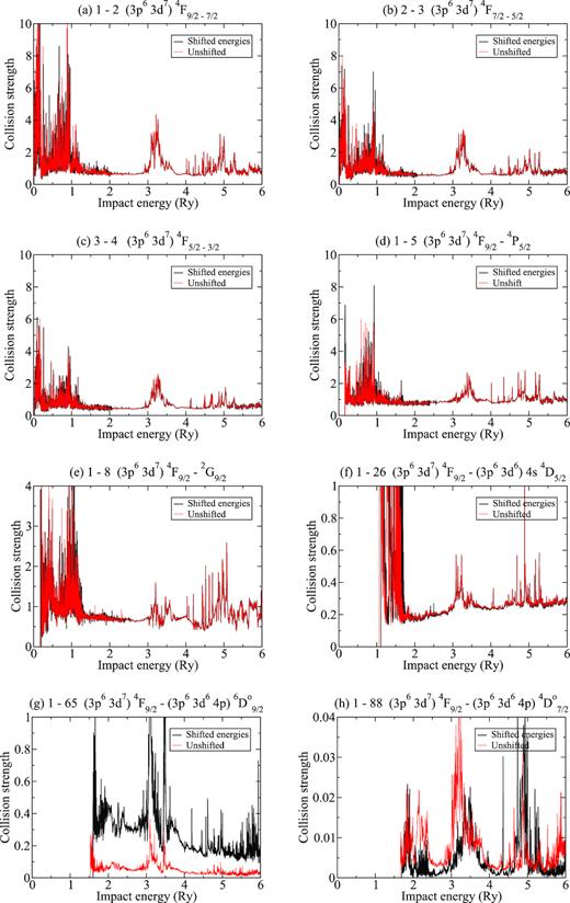
Electron-impact excitation collision strengths Ω of Ni3+.
We present in Fig. 2 the corresponding Maxwellian averaged effective collision strengths Υij for the same transitions depicted in Fig. 1, for a range of electron temperatures |$T_{e} = 10^{3}-10^{6} \, \mathrm{K}$|. Clearly evident is the strong enhancement of the collision rates due to the proper delineation of the Rydberg resonance features in the collision strengths. For the Supporting Information, we provide tables of the calculated effective collision strengths for all the |$34\, 191$| transitions between all levels of Ni3+. For non-Maxwellian modelling or for any application that requires the direct collision strengths we direct the reader to our public ftp server.6 We also refer to the OPEN-ADAS7 data base for the general adf04 file.
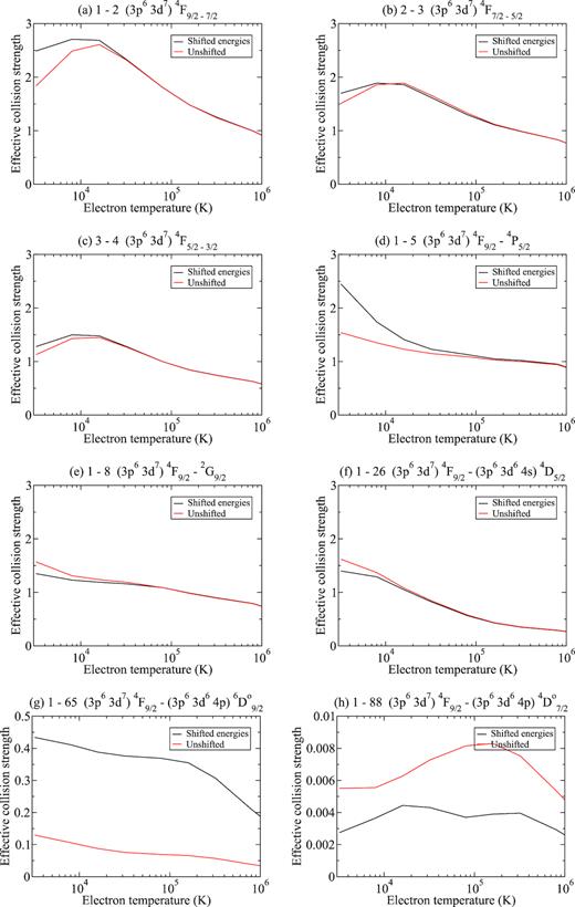
Electron-impact excitation effective collision strengths Υ of Ni3+ for a Maxwellian electron distribution.
As a convergence test we have compared different adf04 files, in the first one we have included in the partial wave expansion angular momenta up to J = 30 and no top-up, in a second one we have added the top-up to the J = 30 expansion, and finally our recommended data with the partial wave expansion extended up to J = 36 plus top-up. The largest differences remain between the versions with and without top-up, in that case the average difference between all the transitions values |$0.5{{\ \rm per\ cent}}$|. In particular for the E1 allowed transitions, the maximum difference reaches the |$100{{\ \rm per\ cent}}$|, while for the forbidden transitions this maximum difference is of the order |$10{{\ \rm per\ cent}}$|. If we add the top-up to the J = 30 expansion the differences reduce significantly, the average difference is reduced to the |$0.02{{\ \rm per\ cent}}$|, and the maximum difference for the E1 transitions to the |$33{{\ \rm per\ cent}}$|, and only in six E1 transitions is above the |$10{{\ \rm per\ cent}}$|, these six transitions are between very excited states, above 100, and they are irrelevant for the modelling. It is clear the calculation is properly converged in terms of the expansion in partial waves once the top-up is added, expansion up to J = 30 and J = 36 produce equal results.
4.2 Photoionization of Ni2+
We have calculated level resolved photoinization cross-sections of Ni2+ from its 20 lowest energy levels for each Jπ symmetry with J = 0–4 and even parity, to all the 262 final states of Ni3+ included in the CC expansion. In a stellar cloud most of the population of Ni2+ will occupy the ground level |$\mathrm{3p^6\, 3d^8\, ^3F_4}$| with only a small fraction populating the metastable levels of the ground term 3F3, 3F2, and 1D2. In an usual stellar cloud these metastable levels contribute to the opacity much less than the ground state. In addition, the 1D2 level is coupled to the 3F term through a spin-changing M1/E2 transition with a very small transition probability. Table 4 shows the Einstein transition coefficients for transitions among the three first terms of Ni2+ taken from Garstang (1958). Clearly transitions between these levels are very weak, with A-values of the order of 10−1–10−2s−1. These levels can therefore be considered as metastable when included in an opacity model. The first odd level of Ni2+ is the |$\mathrm{3p^6\, 3d^7\, 4p\, ^5F_5}$| state, with an excitation energy of |$110\, 213\, \mathrm{cm}^{-1}$| with respect the ground state, see Kramida et al. (2018). All the levels below it are radiatively connected to the ground and metastable states through one or several forbidden E2 and M1 transitions. These transitions are known to be more intense as the level-energy difference is greater and hence terms above 1G will not be populated in a low-density cloud.
Spontaneous emission coefficients for transitions between the lowest excited levels of Ni2+|$\mathrm{3p^6\, 3d^8}$|.
| Lower | Upper | |||
|---|---|---|---|---|
| level | level | Type | WL | A |
| 3F4 | 1D2 | E2 | |$7124.8$| | |$4.5\, [-3]$| |
| 3F3 | 1D2 | M1/E2 | |$7889.9$| | |$4.8\, [-1]$| |
| 3F2 | 1D2 | M1/E2 | |$8499.6$| | |$2.1\, [-1]$| |
| 3F4 | 3P2 | E2 | |$6000.2$| | |$5.0\, [-2]$| |
| 3F3 | 3P1 | E2 | |$6401.5$| | |$3.8\, [-2]$| |
| 3F3 | 3P2 | M1/E2 | |$6533.8$| | |$1.1\, [-1]$| |
| 3F2 | 3P0 | E2 | |$6682.2$| | |$4.6\, [-2]$| |
| 3F2 | 3P1 | M1/E2 | |$6797.1$| | |$1.6\, [-2]$| |
| 3F2 | 3P2 | M1/E2 | |$6946.4$| | |$2.3\, [-2]$| |
| 1D2 | 3P0 | E2 | |$31\, 259$| | |$2.4\, [-6]$| |
| 1D2 | 3P1 | M1/E2 | |$33\, 942$| | |$9.0\, [-2]$| |
| 1D2 | 3P2 | M1/E2 | |$38\, 023$| | |$9.8\, [-2]$| |
Notes. WL, wavelength in air (Å); A, Einstein spontaneous emission coefficient s−1; |$A\, [B]$| denotes A × 10B. Data from Garstang (1958).
In Fig. 3, we present the total photoionization cross-section of Ni2+ from its ground state as a function of photon energy in |$\, \mathrm{Ry}$|, as well as the seven lowest metastable levels. The cross-section depicts a typical structure of large Rydberg resonances on a continuous background. In order to reproduce the high-energy region above approximately |$5.5 \, \mathrm{Ry}$| it is necessary to include more continuum functions and additional highly excited levels in the CC expansion of the target. In the Supporting Information, we provide a full table of fully resolved photoinization cross-sections from the 20 lowest excited levels of with J = 0–4 and even parity of Ni2+ to the 262 lowest-excited levels of Ni3+. These cross-sections can be considered of high-quality for photon energies up to |$5.5 \, \mathrm{Ry}$| and can be used for any opacity model.
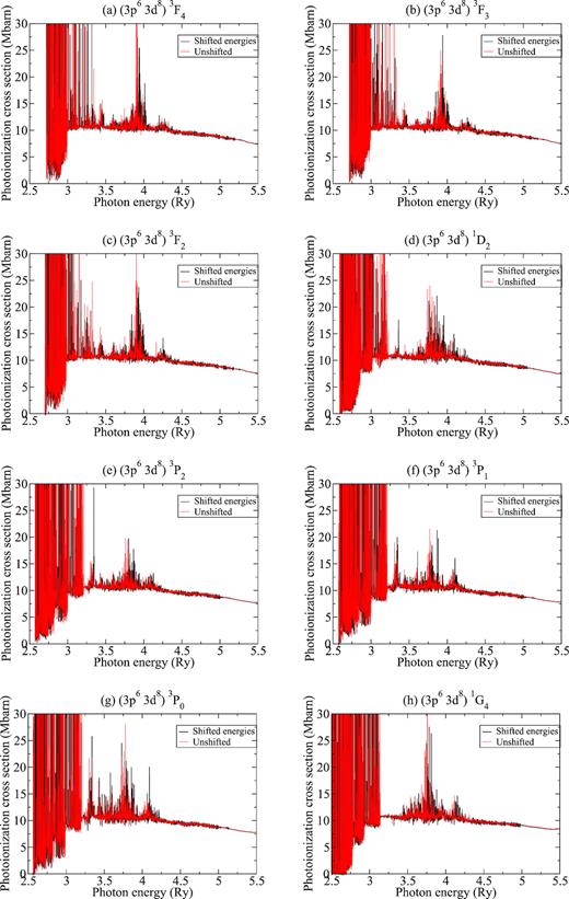
Photoionization cross-sections versus the photon energy for Ni2+ from ground lowest excited initial states. Colour figure is available online.
In Fig. 4, a test of convergence for the calculation is presented. We compare two calculations performed with the same atomic structure of the target. In the first one (black line) we included in the configuration basis set of the (N + 1)-electron system all the configurations derived from the addition of one extra electron into all the available orbitals included in the expansion to those configurations listed in Table 1 and with an expansion of the continuum including Nc = 20 functions. In the second one (red line) the configuration set was reduced somewhat extracting from Table 1 the |$\mathrm{3p^5\, 3d^7\, 5s}$|, |$\mathrm{3p^5\, 3d^7\, 5p}$|, |$\mathrm{3p^5\, 3d^7\, 6s}$|, |$\mathrm{3p^5\, 3d^7\, 6p}$|, |$\mathrm{3p^6\, 3d^5\, 4d^2}$|, |$\mathrm{3p^6\, 3d^6\, 4d}$|, |$\mathrm{3p^4\, 3d^9}$| basis configurations to build the (N + 1)-electron system expansion, and with Nc = 13 functions for the expansion of the continuum. Evidently, there is a very small difference between both calculations with respect to the background, the position of the resonances and their heights. We can be confident therefore that the present calculation has converged with regard to the target description, the size of the continuum basis and the mesh size adopted in the low-energy region. For higher photon energies above |$5.5 \, \mathrm{Ry}$| a similar guarantee of the accuracy of the cross-sections cannot be made due to the effect of additional excited levels which are not included in our CC expansion.
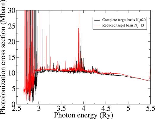
Photoionization cross-section of Ni2+ ion initially in its ground state |$\mathrm{3p^6\, 3d^8\, ^3F_4}$| with two different expansions. Black line, calculation with the whole set of configurations and Nc = 20; Red line, calculation with a truncated set of configurations and Nc = 13.
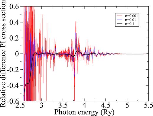
Relative difference of the photoionization cross-section of Ni2+ from its ground level |$\mathrm{3p^6\, 3d^8\, ^3F_4}$| between shifted and unshifted versions of the calculation after several Gaussian convolutions with different widths. Colour figure is available online.
5 MODELLING OF DIAGNOSTICS
With the calculated effective collision strengths for the EIE of Ni3+, we have performed a collision-radiative model. We use the programme colrad, which calculates the line intensities from the radiative transition probabilities and effective collision strengths stored in the adf04 file. For low densities, the only mechanism of population is the collisional excitation from the ground or a metastable state, following radiative-decay cascade. In Table 5, we have selected four line ratios to check their validity as diagnostics. These transitions were considered in a previous calculation by Pradhan & Zhang (1993) for the isoelectronic ion Fe+, and hence provide a benchmark for the current analysis.
Ni iv line ratios used for plasma diagnostics.
| Transition 1 | Transition 2 | ||||
|---|---|---|---|---|---|
| i–j | Levels | WL (Å) | i–j | Levels | WL (Å) |
| 20–21 | 6D9/2–6D7/2 | |$127\, 345$| | 1–2 | 4F9/2–4F7/2 | |$84\, 055$| |
| 1–5 | 4F9/2–4P5/2 | |$5\, 519.2$| | 4–7 | 4F3/2–4P1/2 | |$6\, 121.0$| |
| 1–26 | 4F9/2–4D5/2 | 821.0 | 1–25 | 4F9/2–4D7/2 | 827.1 |
| 1–5 | 4F9/2–4P5/2 | |$5\, 519.2$| | 20–25 | 6D9/2–4D7/2 | |$9\, 524.8$| |
Note. WL, wavelength in vacuum, in Å.
The line intensity ratios are plotted in Fig. 6 as a function of electron temperature and density. The ratio between the lines 1–5 and 20–25 |$(5\, 519.2\, \mathring{\rm A} )/(9\, 524.8\, \mathring{\rm A} )$| provides very powerful diagnostics for the electron temperature T. It is density independent and varies significantly in the range of the peak abundance temperature. The ratio 20–21/1–2 |$(127\, 345\, \mathring{\rm A} )/(84\, 055\, \mathring{\rm A} )$| similarly has a region where it is independent of density but the range is significantly greater than the temperature of maximum abundance for the Ni3+ ion. The ratio between lines 1–26 and 1–25 |$(821.0\, \mathring{\rm A} )/(827.1\, \mathring{\rm A} )$| is a very useful density diagnostic particularly for low-density plasmas, below |$10^{9}\, \mathrm{cm^{-3}}$|, in the range of the temperature of peak abundance. Additional line ratios can be analysed using the present effective collision strengths and with a more refined collision-radiative model. We provide good-quality data to perform plasma modelling using Ni iv emission lines.
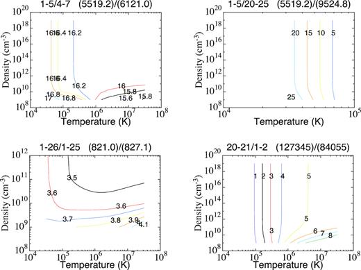
Line intensity ratio |$\frac{I_{\lambda 1}}{I_{\lambda 2}}$| versus electron temperature and density for some selected pairs of lines of Ni iv. Colour online.
For Fe ii, the equivalent wavelengths to the ratio between 1–5 and 20–25 are the lines of |$8\, 617.0$| and |$12\, 566.8\, \mathring{\rm A}$|. The ratio of these lines can give a good diagnostics for the plasma temperature if it is in the range of the peak abundance for Fe+ of |$1.3 \times 10^{4} \, \mathrm{K}$|, see (Smyth et al. 2019). Combining these two line ratios for Fe ii and Ni iv, we are able to determine with accuracy the electron temperature of the plasma in a wider range. In Fig. 7, we show the variation of these line ratios for the electron density of the Orion nebula.
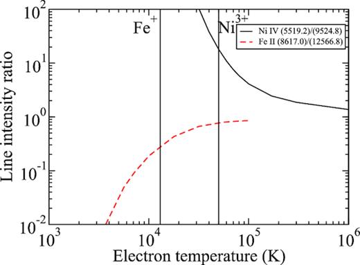
Line intensity ratio |$\frac{I_{\lambda 1}}{I_{\lambda 2}}$| versus electron temperature for a constant density of |$d=10^{4}\, \mathrm{cm}^{-3}$| for lines |$(5\, 519.2\, \mathring{\rm A} )/(9\, 524.8\, \mathring{\rm A} )$| of Ni iv (full line) and |$(8\, 617.0\, \mathring{\rm A} )/(12\, 566.8\, \mathring{\rm A} )$| of Fe ii (dashed line). Vertical lines indicate the peak abundance temperature of each ion. Colour figure is available online.
6 CONCLUSIONS
We present high-quality atomic data for EIE of Ni3+ and photoionization from the ground and metastable levels of Ni2+. These data are essential for the interpretation of Ni iv lines collected from ground and satellite observations, as well as opacity due to Ni2+ in interstellar clouds. A fully relativistic darc treatment is adopted with a configuration interaction expansion of the 25-electron target Ni3+ incorporating lowest 262 levels in the close coupling expansion of the target. For each of the two processes, we have performed two calculations, one using the calculated energies and atomic wave functions obtained within grasp, and a second one replacing the calculated energies with the recommended data tabulated in the NIST database. For both processes, the differences between the two calculations performed were negligible with the background cross-section as well as the height and positioning of the resonance structures almost identical in both. Accuracy checks were performed throughout the analysis and we are confident that the present data represent the best available to date for use by the astrophysics and plasma physics communities.
SUPPORTING INFORMATION
energies.dat
radiative.dat
upsilon.dat
Please note: Oxford University Press is not responsible for the content or functionality of any supporting materials supplied by the authors. Any queries (other than missing material) should be directed to the corresponding author for the article.
ACKNOWLEDGEMENTS
Present work has been funded by the Science and Technology Facility Council (STFC) through the Queen's University Belfast (QUB) Astronomy Observation and Theory Consolidated Grant ST/P000312/1. The computation has been performed in the supercomputer Hazelhen property of the Höchstleistungsrechner für Wissenschaft und Wirtschaft (Germany), and Archer property of the Engineering and Physical Science Research Council under the allocation E464-RAMPA.
