


ABSTRACT
We study the morphological and structural properties of the host galaxies associated with 57 optically selected luminous type 2 active galactic nuclei (AGNs) at |$z$| ∼ 0.3–0.4: 16 high-luminosity Seyfert 2 [HLSy2, 8.0 ≤ log(|$L_{\rm [O\,{\small III}]}/L_{\odot })\,\lt\,$| 8.3] and 41 obscured [QSO2, log(|$L_{\rm [O\,{\small III}]}/L_{\odot })\ge$| 8.3] quasars. With this work, the total number of QSO2s at |$z$| < 1 with parametrized galaxies increases from ∼35 to 76. Our analysis is based on Hubble Space Telescope WFPC2 and ACS images that we fit with galfit. HLSy2s and QSO2s show a wide diversity of galaxy hosts. The main difference lies in the higher incidence of highly disturbed systems among QSO2s. This is consistent with a scenario in which galaxy interactions are the dominant mechanism triggering nuclear activity at the highest AGN power. There is a strong dependence of galaxy properties with AGN power (assuming |$L_ {\rm [O\,{\small III}]}$| is an adequate proxy). The relative contribution of the spheroidal component to the total galaxy light (B/T) increases with |$L_ {\rm [O\,{\small III}]}$|. While systems dominated by the spheroidal component spread across the total range of |$L_ {\rm [O\,{\small III}]}$|, most disc-dominated galaxies concentrate at log(|$L_{\rm [O\,{\small III}]}/L_{\odot })\lt$|8.6. This is expected if more powerful AGNs are powered by more massive black holes which are hosted by more massive bulges or spheroids. The average galaxy sizes (〈re〉) are 5.0 ± 1.5 kpc for HLSy2s and 3.9 ± 0.6 kpc for HLSy2s and QSO2s, respectively. These are significantly smaller than those found for QSO1s and narrow-line radio galaxies at similar |$z$|. We put the results of our work in the context of related studies of AGNs with quasar-like luminosities.
1 INTRODUCTION
Studies of the host galaxies associated with active galactic nuclei (AGNs) are relevant to a diversity of topics related to galaxy formation and evolution, such as what mechanisms control nuclear activity and supermassive black hole (SMBH) growth in galaxies? What is the role of orientation and obscuration in the observed differences among certain AGN sub-classes? How is radio activity triggered? What is the origin of the tight scaling relations between the SMBH masses and various properties of their host spheroids? Ultimately, what is the link between galaxy and SMBH formation and evolution?
Quasars are the most powerful active galaxies. By studying their host galaxies at different redshifts (|$z$|) we can investigate how the most massive black holes form and evolve, what mechanisms trigger the most extreme form of nuclear activity, and how this can affect the evolution of massive galaxies (Kormendi & Richstone 1995; Magorrian et al. 1998; Ferrarese & Merritt 2000; Gebhardt et al. 2000; Tremaine et al. 2002). Such studies have been focused traditionally on type 1 (unobscured) quasars (QSO1s). While some of the works proposed that QSO1s at low redshift (|$z$| < 0.5) are almost invariably hosted by massive bulge-dominated galaxies (McLeod & Rieke 1994, 1995b; Dunlop et al. 2003; Lacy 2006; Hyvönen et al. 2007), other studies have shown a large diversity of hosts. A substantial disc component has been found in many galaxies hosting low-|$z$| quasars, with the relative contribution to the total galaxy light possibly dependent on the quasar luminosity and radio loudness (Bahcall et al. 1997; Floyd et al. 2004; Jahnke, Kuhlbrodt & Wisotzki 2004; Bettoni et al. 2015).
In regard to the physical mechanisms that trigger AGN activity and SMBH growth, there is evidence that a variety of processes can be involved, with the dominant one depending on AGN luminosity. While mergers of gas-rich galaxies are frequently suggested as the trigger for quasars, secular processes appear to be more relevant at lower AGN power (Toomre & Toomre 1972; Heckman et al. 1986; Combes 2001; Hopkins et al. 2006; Cisternas et al. 2011; Ramos-Almeida et al. 2011; Bessiere et al. 2012).
Host galaxy studies of type 2 (obscured) QSOs (QSO2s) at different |$z$| are currently of special relevance. This population is at least comparable in number density to the QSO1 population and perhaps two to three times larger (Tajer 2007; Gilli et al. 2011; Mateos et al. 2017). They are of great interest since they are signposts of vigorous obscured SMBH growth.
In comparison with QSO1 studies, they can provide useful information regarding the QSO1 versus QSO2 unification scenario based on orientation (Antonucci 1993).
Only ∼10–15 per cent of quasars are radio-loud. This applies to both QSO1s (Katgert et al. 1973; Fanti et al. 1977; Smith & Wright 1980) and QSO2s (Lal & Ho 2010). QSO2 studies offer the opportunity to characterize the host galaxies of the most luminous obscured radio-quiet AGNs versus their radio-loud analogues, narrow-line radio galaxies (NLRGs; e.g. Dunlop et al. 2003; Best et al. 2005; Inskip et al. 2010).
QSO2s have been discovered in large numbers only recently (Zakamska et al. 2003). For this reason, studies of their hosts are scarce and have been focused on small samples. Such studies have a clear advantage with respect to QSO1s: The obscuration of the central engine renders a detailed view of the galaxies, allowing a more accurate morphological and structural characterization. These works suggest a diversity of galaxy host types, with a clear preference for ellipticals and bulge-dominated systems (Greene et al. 2009, Bessiere et al. 2012; Kocevski et al. 2012; Villar Martín et al. 2012; Wylezalek et al. 2016).
With the goal of shedding more light on this topic, we present here the results of the morphological and parametric characterization and subsequent classification of the host galaxies associated with 57 luminous obscured AGNs at |$z$| ∼ 0.3–0.4. Forty-one are QSO2s. In order to investigate the potential dependence of galaxy host properties with AGN power, 16 high-luminosity Seyfert 2 (HLSy2) galaxies are also part of this study (McLeod & Rieke 1995a; Kauffmann et al. 2003).
We also identify and classify merger/interaction features. Our study is based on Hubble Space Telescope (HST) optical images obtained with the Advanced Camera for Surveys/Wide Field Channel (ACS/WFC) and the Wide Field Planetary Camera 2 (WFPC2). We have applied two different techniques: a visual classification and multiparametric modelling, using galfit (Peng et al. 2010), which allows us to isolate and parametrize the galaxy structural components.
The paper is organized as follows. The AGN sample and data are described in Section 2. The classification methods and the modelling procedure are explained in Section 3. The results of the visual and parametric classifications are presented in Section 4 and discussed in the context of related works in Section 5. Summary and conclusions are in Section 6.
We assume |$\Omega _\Lambda = 0.73$|, ΩM = 0.27, and H0 =71 km s−1 Mpc−1.
2 SAMPLE AND DATA
The sample studied here consists of 57 luminous (lO3 = log(|$L_{\rm [O\,{\small III}]}/L_{\odot })\ge$| 8.0) type 2 AGNs at 0.3 < |$z$| < 0.4 from Zakamska et al. (2003) and Reyes et al. (2008) catalogues of Sloan Digital Sky Survey (SDSS) luminous type 2 AGNs (Table 1).
List of objects observed for the HST programme 10880. Column (3) quotes the kpc arcsec−1 conversion. The [O iii] luminosity in column (4), lO3, is given in log and relative to the solar luminosity (Reyes et al. 2008). Objects with lO3 ≳ 8.3 are QSO2s in column (7). Objects with lower values are classified as HLSy2s. Column (5): HST instrument and filter. Column (6): date of observation. Column (8): emission lines contaminating the filter.
| Object | z | Scale | lO3 | Instrument | Date | AGN | Emission lines |
|---|---|---|---|---|---|---|---|
| SDSS name | (kpc arcsec−1) | /filter | yr/mm/dd | classification | |||
| [1] | [2] | [3] | [4] | [5] | [6] | [7] | [8] |
| J002531.46−104022.2 | 0.303 | 4.45 | 8.73 | ACS/F775W | 06/09/11 | QSO2 | H α, [N ii] doublet |
| J005515.82−004648.6 | 0.345 | 4.86 | 8.15 | WFPC2/F814W | 07/06/18 | HLSy2 | H α, [N ii] doublet |
| J011429.61+000036.7 | 0.389 | 5.25 | 8.66 | ACS/F775W | 06/08/07 | QSO2 | [O iii] 4959,5007 |
| J011522.19+001518.5 | 0.390 | 5.26 | 8.14 | WFPC2/F814W | 07/06/11 | HLSy2 | H α, [N ii] doublet |
| J014237.49+144117.9 | 0.389 | 5.25 | 8.76 | ACS/F775W | 06/08/11 | QSO2 | [O iii] 4959,5007 |
| J015911.66+143922.5 | 0.319 | 4.61 | 8.56 | ACS/F775W | 06/08/12 | QSO2 | No |
| J020234.56−093921.9 | 0.302 | 4.44 | 8.39 | WFPC2/F814W | 07/06/18 | QSO2 | H α, [N ii] doublet |
| J021059.66−011145.5 | 0.384 | 5.21 | 8.10 | WFPC2/F814W | 07/06/25 | HLSy2 | H α, [N ii] doublet |
| J021758.18−001302.7 | 0.344 | 4.85 | 8.55 | ACS/F775W | 06/10/19 | QSO2 | No |
| J021834.42−004610.3 | 0.372 | 5.10 | 8.85 | ACS/F775W | 06/09/15 | QSO2 | [O iii] 5007 |
| J022701.23+010712.3 | 0.363 | 5.02 | 8.90 | ACS/F775W | 06/11/06 | QSO2 | [O iii] 5007 |
| J023411.77−074538.4 | 0.310 | 4.52 | 8.77 | ACS/F775W | 06/10/30 | QSO2 | H α, [N ii] doublet |
| J031946.03−001629.1 | 0.393 | 5.22 | 8.24 | WFPC2/F814W | 08/11/25 | HLSy2 | H α, [N ii] doublet |
| J031927.22+000014.5 | 0.385 | 5.28 | 8.06 | WFPC2/F814W | 08/11/25 | HLSy2 | H α, [N ii] doublet |
| J032029.78+003153.5 | 0.384 | 5.21 | 8.52 | ACS/F775W | 06/11/11 | QSO2 | [O iii] 4959, 5007 |
| J032533.33−003216.5 | 0.352 | 4.93 | 9.06 | WFPC2/F814W | 08/11/26 | QSO2 | H α, [N ii] doublet |
| J033310.10+000849.1 | 0.327 | 4.69 | 8.13 | WFPC2/F814W | 08/11/25 | HLSy2 | H α, [N ii] doublet |
| J034215.08+001010.6 | 0.348 | 4.89 | 9.08 | WFPC2/F814W | 08/11/22 | QSO2 | H α, [N ii] doublet |
| J040152.38−053228.7 | 0.320 | 4.62 | 8.96 | WFPC2/F814W | 08/11/28 | QSO2 | H α, [N ii] doublet |
| J074811.44+395238.0 | 0.372 | 5.10 | 8.19 | WFPC2/F814W | 08/11/20 | HLSy2 | H α, [N ii] doublet |
| J081125.81+073235.3 | 0.350 | 4.91 | 8.88 | WFPC2/F814W | 08/11/22 | QSO2 | H α, [N ii] doublet |
| J081330.42+320506.0 | 0.398 | 5.33 | 8.83 | ACS/F775W | 06/12/16 | QSO2 | [O iii] 4959, 5007 |
| J082449.27+370355.7 | 0.305 | 4.47 | 8.28 | WFPC2/F814W | 08/11/23 | QSO2 | H α, [N ii] doublet |
| J082527.50+202543.4 | 0.336 | 4.78 | 8.88 | WFPC2/F814W | 08/11/20 | QSO2 | Hα, [N ii] doublet |
| J083028.14+202015.7 | 0.344 | 4.85 | 8.91 | WFPC2/F814W | 08/11/20 | QSO2 | H α, [N ii] doublet |
| J084041.08+383819.8 | 0.313 | 4.55 | 8.47 | WFPC2/F814W | 08/11/21 | QSO2 | H α, [N ii] doublet |
| J084309.86+294404.7 | 0.397 | 5.32 | 9.34 | WFPC2/F814W | 08/11/21 | QSO2 | [O iii] 5007, H α, [N ii] doublet |
| J084856.58+013647.8 | 0.350 | 4.91 | 8.46 | ACS/F775W | 06/10/08 | QSO2 | No |
| J084943.82+015058.2 | 0.376 | 5.14 | 8.06 | WFPC2/F814W | 08/11/26 | HLSy2 | H α, [N ii] doublet |
| J090307.84+021152.2 | 0.329 | 4.71 | 8.42 | WFPC2/F814W | 08/11/26 | QSO2 | H α, [N ii] doublet |
| J090414.10−002144.9 | 0.353 | 4.94 | 8.93 | ACS/F775W | 06/12/11 | QSO2 | No |
| J090801.32+434722.6 | 0.363 | 5.02 | 8.31 | WFPC2/F814W | 08/11/21 | QSO2 | H α, [N ii] doublet |
| J092318.06+010144.8 | 0.386 | 5.23 | 8.94 | WFPC2/F814W | 08/11/21 | QSO2 | H α, [N ii] doublet |
| J092356.44+012002.1 | 0.380 | 5.17 | 8.59 | WFPC2/F814W | 08/11/17 | QSO2 | H α, [N ii] doublet |
| J094209.00+570019.7 | 0.350 | 4.91 | 8.31 | WFPC2/F814W | 08/11/22 | QSO2 | H α, [N ii] doublet |
| J094350.92+610255.9 | 0.341 | 4.82 | 8.46 | WFPC2/F814W | 07/04/15 | QSO2 | H α, [N ii] doublet |
| J095629.06+573508.9 | 0.361 | 5.01 | 8.38 | WFPC2/F814W | 08/11/26 | QSO2 | H α, [N ii] doublet |
| J100329.86+511630.7 | 0.324 | 4.66 | 8.11 | WFPC2/F814W | 08/11/26 | HLSy2 | H α, [N ii] doublet |
| J103639.39+640924.7 | 0.398 | 5.33 | 8.42 | WFPC2/F814W | 07/04/14 | QSO2 | [O iii] 5007, H α, [N ii] doublet |
| J112907.09+575605.4 | 0.313 | 4.55 | 9.38 | WFPC2/F814W | 08/11/26 | QSO2 | H α, [N ii] doublet |
| J113710.78+573158.7 | 0.395 | 5.30 | 9.61 | WFPC2/F814W | 08/11/26 | QSO2 | [O iii] 5007, H α, [N ii] doublet |
| J133735.01−012815.7 | 0.329 | 4.71 | 8.72 | WFPC2/F814W | 07/04/04 | QSO2 | H α, [N ii] doublet |
| J140740.06+021748.3 | 0.309 | 4.51 | 8.90 | WFPC2/F814W | 07/04/05 | QSO2 | H α, [N ii] doublet |
| J143027.66−005614.9 | 0.318 | 4.60 | 8.44 | WFPC2/F814W | 07/04/05 | QSO2 | H α, [N ii] doublet |
| J144711.29+021136.2 | 0.386 | 5.23 | 8.45 | WFPC2/F814W | 07/05/02 | QSO2 | H α, [N ii] doublet |
| J150117.96+545518.3 | 0.338 | 4.79 | 9.06 | WFPC2/F814W | 07/04/08 | QSO2 | H α, [N ii] doublet |
| J154133.19+521200.1 | 0.311 | 4.53 | 8.25 | WFPC2/F814W | 07/04/02 | HLSy2 | H α, [N ii] doublet |
| J154337.81−004420.0 | 0.311 | 4.53 | 8.40 | WFPC2/F814W | 07/05/05 | QSO2 | H α, [N ii] doublet |
| J154613.27−000513.5 | 0.383 | 5.20 | 8.18 | WFPC2/F814W | 07/05/03 | HLSy2 | H α, [N ii] doublet |
| J172419.89+551058.8 | 0.365 | 5.04 | 8.00 | WFPC2/F814W | 07/05/17 | HLSy2 | H α, [N ii] doublet |
| J172603.09+602115.7 | 0.333 | 4.75 | 8.57 | WFPC2/F814W | 07/04/08 | QSO2 | H α, [N ii] doublet |
| J173938.64+544208.6 | 0.384 | 5.21 | 8.42 | WFPC2/F814W | 07/04/10 | QSO2 | H α, [N ii] doublet |
| J214415.61+125503.0 | 0.390 | 5.26 | 8.14 | WFPC2/F814W | 07/05/14 | HLSy2 | Hα, [N ii] doublet |
| J215731.40+003757.1 | 0.390 | 5.26 | 8.39 | WFPC2/F814W | 07/05/12 | QSO2 | H α, [N ii] doublet |
| J223959.04+005138.3 | 0.384 | 5.21 | 8.15 | WFPC2/F814W | 07/05/17 | HLSy2 | H α, [N ii] doublet |
| J231755.35+145349.4 | 0.311 | 4.53 | 8.10 | WFPC2/F814W | 07/05/21 | HLSy2 | H α, [N ii] doublet |
| J231845.12−002951.4 | 0.397 | 5.32 | 8.00 | WFPC2/F814W | 07/06/12 | HLSy2 | [O iii] 5007, H α, [N ii] doublet |
Zakamska et al. (2003) selected 291 luminous type 2 AGNs (lO3 > 7.3), at |$z$| < 0.83, from SDSS on the basis of their optical emission-line properties: narrow emission lines (full width at half-maximum, FWHM < 2000 km s−1) without underlying broad components and optical line ratios typical of active galaxies, consistent with non-stellar ionizing radiation. Reyes et al. (2008) updated this catalogue based on ∼3 times as much SDSS data. Their catalogue contains 887 luminous type 2 AGNs (lO3 > 7.9), recovering >90 per cent of objects in Zakamska et al. (2003) in the same luminosity range. The spectra of the objects they missed tend to have low S/N or ambiguous classification.
About 744 (84 per cent) objects in Reyes et al. (2008) have lO3 ≥ 8.3 and are, therefore, QSO2s. This threshold ensures the selection of objects with AGN luminosities in the quasar regime. Using |$L_ {\rm [O\,{\small III}]}$| as a proxy for AGN power (Heckman et al. 2004), the implied bolometric luminosities are above the classical Seyfert/quasar separation of Lbol ∼ 1045 erg s−1. Only ∼15 per cent ± 5 per cent QSO2s are expected to be radio-loud (Lal & Ho 2010).
The 57 AGNs studied here are the sample of objects observed for theHST programme 10880, with principal investigator Henrique Schmitt (Tables 1 and 2). HST imaging observations for other programmes exist for several more QSO2s, but in general they have been done with different filters and/or the targets are at different |$z$| than our sample. Since the statistics will not improve significantly, these are not considered in our study.
Instrument specifications. Column (4): range of point spread function (PSF) physical sizes spanned by the |$z$| of the sample. Column (6): spectral range covered by the filter. Column (7): zero-point values for flux calibration (Lucas et al. 2016). Column (8): number of objects observed with each instrument.
| Instrument | Pixel scale | FWHM (PSF) | FWHM (PSF) | Filter | Δλ | Zp | No. of objects |
|---|---|---|---|---|---|---|---|
| (arcsec pix−1) | (arcsec) | (kpc) | (Å) | ||||
| [1] | [2] | [3] | [4] | [5] | [6] | [7] | [8] |
| ACS/WFC | 0.05 | 0.12 | 0.54–0.65 | F775W | 6804–8632 | 25.65 | 12 |
| WFCP2 | 0.1 | 0.25 | 1.1–1.4 | F814W | 6984–10043 | 24.21 | 45 |
There are 97 SDSS QSO2s and 36 HLSy2s in the 0.3 < |$z$| < 0.4 range. Of these, our sub-sample contains 41 (∼42 per cent) QSO2s and 16 HLSy2s (∼44 per cent). Although uncertainties remain regarding the exact selection criteria applied by the team responsible for the 10880 HST programme, based on the high fractions quoted above we consider they are an adequate representation of the total sample of SDSS QSO2s and HLSy2s in these |$z$| and |$L_{\rm [O\,{\small III}]}$| ranges.
The ACS/WFC and WFPC2 images used in this work are from the Hubble Legacy Archive (HLA).1
3 CLASSIFICATION METHODS
We have classified the host galaxies based on two main methods: visual and parametric.
The visual inspection of host galaxy images provides a classification based on their apparent morphology. It has been a standard practice for more than eighty years (Hubble 1936) and is still contributing today to achieve a deeper understanding of galaxy evolution (Lintott 2008; Nair & Abraham 2010; Willett et al. 2013). A limitation of this method is that it can be subjective, so the same object can be classified differently by different observers. Frequently, it does not allow one to determine which structural component (disc or bulge) dominates the total galaxy light, thus preventing an accurate classification. A more robust classification needs to be based on a multiparametric modelling approach. This allows one to extract structural components from galaxy images, by modelling their light profiles (Peng et al. 2010). This method also has limitations. For example, complex mergers can be misclassified by applying a too simplistic approach assuming that all galaxies consist of a disc and/or a spheroidal component. Visual inspection is particularly useful in these cases.
Both methods have been essential in our work: The visual classification has allowed us to identify complex mergers that cannot be classified as either bulge- or disc-dominated systems. It has also been useful to disentangle the parametric classification in a minority of bulge- or disc-dominated cases where the parametric method resulted in degenerate fits.
More details of the classification methods are provided next.
3.1 Visual classification
We have applied three different methods of visual classification:
Method Vis-I. Three groups have been considered: spiral and discs without obvious spiral arms, ellipticals, and highly disturbed systems. These are systems of very complex morphologies due to merger/interaction processes that cannot be classified in the previous two groups.
Method Vis-II. This focuses on the identification of features indicative of galaxy interactions.
Given that QSO2 host galaxies are often associated with morphological features indicative of past or ongoing merger/interaction events (Bessiere et al. 2012; Villar Martín et al. 2012), we have classified our objects to highlight the presence of such features, adopting the following schemes of Rodríguez Zaurín et al. (2011) and Veilleux, Kim & Sanders (2002):
Class 0: objects that appear to be single isolated galaxies, dominated by a relatively symmetric morphology with no peculiar features.
Class 0*: objects that appear to be single isolated galaxies, dominated by a symmetric morphology with some faint irregular morphological features such as tails and shells (see Method Vis-III below).
Class 1: objects in a pre-coalescence phase with two well-differentiated nuclei separated by a projected distance >1.5 kpc. For these objects, it is still possible to identify the individual merging galaxies and their corresponding tidal structures due to the interaction.
Class 2: objects with two nuclei separated by a projected distance ≤1.5 kpc or a single nucleus with an asymmetric morphology and prominent irregular features suggesting a post-coalescence merging phase.
Method Vis-III. This focuses on morphological appearance of peculiar features. To further refine this classification, we have also characterized the morphological appearance of the merger/interaction features following Ramos-Almeida et al. (2011) – T: tidal tail; F: fan; B: bridge; S: shell; D: dust feature; 2N: dual-core/double nucleus; A: amorphous halo; I: irregular feature; IC: interacting companion. We have added the following as an extra feature – K: knot.
In this paper, we present the results of all three visual methods, although we will focus the scientific discussion on Method Vis-I.
3.2 Parametric classification
galfit fits the following parameters for each Sérsic component: central position (x, y), integrated magnitude (MAG),2re, n, axial ratio (b/a), and position angle of the major axis (PA). The users need to start the algorithm with initial guesses for these parameters, which have to be as accurate as possible, and a value for the sky background. Following different works (Häußler al. 2007; Buitrago et al. 2008, 2017), we obtain the input parameters with SExtractor (Bertin & Arnouts 1996) except the sky background (see Section 3.2.2). Zero-points are fixed in each object, and they are provided in Table 2. Close neighbours were fitted using single Sérsic profiles simultaneously with the target galaxies to avoid contamination of the AGN host light profiles.
galfit provides re and MAG of the individual components, but not the global values for the galaxy. To obtain these, elliptical isophotes were fitted to the galaxy’s 2D model using the ELLIPSE task in iraf. To avoid overestimations of the total galaxy flux FT and of re, the outer model isophote was carefully fixed to coincide with the HST image isophote for which the flux per pixel is >3σ (Section 3.2.2). The relative contribution of each structural component is measured as the flux within this isophote relative to FT, |$\frac{F_{\rm i}}{F_{\rm T}}$|. The galaxy re is taken as the major axis of the model isophote that contains |$\frac{F_{\rm T}}{2}$| (Table 3).
Comparison between the total magnitude and the half-radius calculated with SExtractor and the effective radius inferred with the task ellipse applied to the galfit 2D model image. Only objects that could be fitted with galfit are shown. The SExtractor values were obtained by applying the code to the HST data. The galfit mag and Reff values were measured in the best-fitting model image.
| Object | lO3 | Magnitude (mag) | Hr SExtractor | Reffgalfit | |
|---|---|---|---|---|---|
| SDSS name | SExtractor | galfit | (kpc) | (kpc) | |
| [1] | [2] | [3] | [4] | [5] | [6] |
| J005515.82−004648.6 | 8.15 | 19.3 | 19.3 | 1.5 | 1.5 |
| J011429.61+000036.7 | 8.66 | 17.7 | 17.5 | 5.5 | 5.9 |
| J011522.19+001518.5 | 8.14 | 18.1 | 18.1 | 7.8 | 4.5 |
| J014237.49+144117.9 | 8.76 | 17.8 | 17.8 | 1.1 | 1.1 |
| J015911.66+143922.5 | 8.56 | 19.7 | 19.5 | 1.4 | 1.2 |
| J020234.56−093921.9 | 8.39 | 17.4 | 17.6 | 7.1 | 6.3 |
| J021059.66−011145.5 | 8.10 | 19.0 | 19.0 | 3.8 | 3.0 |
| J023411.77−074538.4 | 8.77 | 18.7 | 18.7 | 2.2 | 2.3 |
| J031946.03−001629.1 | 8.06 | 18.9 | 18.8 | 6.3 | 7.5 |
| J031927.22+000014.5 | 8.24 | 19.1 | 18.8 | 4.2 | 4.5 |
| J032029.78+003153.5 | 8.52 | 17.3 | 17.0 | 10.0 | 12.8 |
| J034215.08+001010.6 | 9.08 | 19.3 | 19.2 | 1.2 | 1.1 |
| J040152.38−053228.7 | 8.96 | 18.9 | 19.0 | 2.8 | 2.7 |
| J074811.44+395238.0 | 8.19 | 18.9 | 18.7 | 4.5 | 4.6 |
| J081125.81+073235.3 | 8.88 | 19.1 | 19.2 | 5.5 | 4.0 |
| J082449.27+370355.7 | 8.28 | 19.2 | 19.0 | 1.2 | 1.3 |
| J082527.50+202543.4 | 8.88 | 19.7 | 19.7 | 0.9 | 1.1 |
| J083028.14+202015.7 | 8.91 | 18.6 | 18.5 | 2.2 | 2.5 |
| J084041.08+383819.8 | 8.47 | 17.9 | 17.8 | 6.3 | 7.1 |
| J084309.86+294404.7 | 9.34 | 18.8 | 18.7 | 3.9 | 3.1 |
| J084856.58+013647.8 | 8.46 | 17.8 | 17.1 | 6.1 | 4.9 |
| J084943.82+015058.2 | 8.06 | 19.5 | 19.5 | 1.9 | 2.2 |
| J090414.10−002144.9 | 8.93 | 17.9 | 17.8 | 2.8 | 2.9 |
| J092318.06+010144.8 | 8.94 | 18.9 | 18.8 | 3.6 | 3.1 |
| J094209.00+570019.7 | 8.31 | 18.9 | 18.7 | 1.8 | 1.6 |
| J094350.92+610255.9 | 8.46 | 19.5 | 19.6 | 1.0 | 1.0 |
| J095629.06+573508.9 | 8.38 | 19.1 | 19.0 | 2.8 | 3.2 |
| J100329.86+511630.7 | 8.11 | 18.4 | 18.4 | 5.2 | 4.8 |
| J103639.39+640924.7 | 8.42 | 18.1 | 17.8 | 7.5 | 7.3 |
| J112907.09+575605.4 | 9.38 | 19.3 | 19.1 | 2.0 | 2.4 |
| J113710.78+573158.7 | 9.61 | 19.1 | 18.6 | 3.0 | 3.3 |
| J140740.06+021748.3 | 8.90 | 19.3 | 19.2 | 1.4 | 1.5 |
| J150117.96+545518.3 | 9.06 | 17.2 | 17.2 | 6.2 | 6.1 |
| J154133.19+521200.1 | 8.25 | 17.8 | 18.0 | 7.9 | 6.7 |
| J154613.27−000513.5 | 8.18 | 19.3 | 19.0 | 3.8 | 3.8 |
| J172419.89+551058.8 | 8.00 | 19.5 | 19.3 | 1.5 | 1.4 |
| J172603.09+602115.7 | 8.57 | 19.8 | 19.8 | 1.2 | 1.2 |
| J173938.64+544208.6 | 8.42 | 19.3 | 19.2 | 2.1 | 2.6 |
| J214415.61+125503.0 | 8.14 | 18.4 | 18.5 | 1.9 | 1.2 |
| J223959.04+005138.3 | 8.15 | 18.9 | 18.9 | 3.7 | 3.6 |
| J231755.35+145349.4 | 8.10 | 18.4 | 18.3 | 6.7 | 6.2 |
| J231845.12D−002951.4 | 8.00 | 18.6 | 18.4 | 5.6 | 4.3 |
3.2.1 PSF
We refer the reader to Appendix A for a detailed description and discussion on the PSF construction method.
3.2.2 Determination of the sky background
An accurate determination of the sky background is essential, especially for faint objects and galaxies with extended low surface brightness structures.
Following Häußler al. (2007) we introduced the background level as a fixed parameter of galfit. To calculate it for each AGN image, we selected emission-free areas (i.e. masking sources) around the object to avoid contamination. The sky background was then estimated as the average value of all pixels with values <3σ, after applying a 3σ clipping method.
3.2.3 Methodology
We have followed two steps to obtain the parametric fits:
Method Par-I. The light profile and global morphology are parametrized using a single Sérsic component. This method has been used in numerous works (Weinzirl et al. 2009; Buitrago et al. 2013; Davari, Ho & Peng 2016) to classify galaxies depending on n into spheroidal or disc galaxies.
As we will see (Section 4.2), single Sérsic profiles do not provide acceptable fits in the majority of our objects. This method has been useful, on the other hand, to obtain a preliminary guess of the galaxy types and to constrain the input parameters of galfit when applying more complex fits (Method Par-II). It has also proved useful to identify objects where the contribution of a point source is necessary. It is found that whenever a single Sérsic component fit resulted on an n ≥8, the contribution of a point source is confirmed by the more sophisticated Method Par-II. The point source contribution may be relatively low in flux, but it can modify the shape of the inner light profile significantly.
Method Par-II. Two or more components are considered in the fit with the goal of isolating and parametrizing different constituents and, when necessary, to separate overlapping galaxies. The combination can include two or more Sérsic components and, if necessary, a point source. All are combined to reproduce the global light profile of a given galaxy.
For a given object, we select the fit with the minimum number of components that best reproduces the surface brightness profile and leaves minimum residuals in the 2D residual image, excluding asymmetric peculiar features. We find that all galaxies can be successfully fitted with a maximum of three components: a point source and two Sérsic profiles.
3.2.4 Physical nature of the structural components
One of our main aims is to classify the galaxies according to the structural component that dominates the galaxy luminosity (i.e. bulge-dominated, disc-dominated, other). It is necessary to define some criteria to associate each component with a physical counterpart.
We assume n =1 for discs. This is a common practice, which is justified by the fact that the light profile of discs is indeed exponential (Freeman 1970). The situation is less simple for bulges and elliptical galaxies. Although the r1/4 de Vaucouleurs profile (de Vaucouleurs 1959) is often assumed, numerous works have shown that this must be generalized to r1/n to account for the range of values of n spanned by different galaxies (Trujillo et al. 2001; Allen et al. 2006; Häußler al. 2007; Ribeiro et al. 2016). Following Gadotti (2009) (see also Barentine & Kormendy 2012) we will consider that an n ≥ 2 Sérsic is a bulge.
Peculiar features are frequent around high-luminosity AGNs (e.g. tidal tails and fans). This is also the case for our sample (Villar Martín et al. 2012; see also 4.1.2). When such features are irregular and asymmetric, they are easily recognized in the residual images. However, when they are diffuse and symmetric, galfit may reproduce them successfully with low n ≤1 Sérsic components, which may be erroneously interpreted as discs or bars (n ∼ 0.5; Peng et al. 2002). To avoid such degeneracy (which we find to affect a minority of objects anyway), we have carefully checked for every target whether the interpretation of the nature of the different structural components revealed by the fit is coherent with the visual inspection.
Taking into account all these considerations, the galaxies will be classified as follows:
Highly disturbed systems. This group contains objects with strongly distorted morphologies with clear signs of galactic interactions, according to the classification described in Section 3.1. These objects cannot be fitted with galfit accurately.
Point-source-dominated objects. A point source contributes >50 per cent to the total galaxy flux.
Objects with a single Sérsic component (with or without point source). The objects will be classified in terms of n following Graham et al. (2005; see also Häußler al. 2007).
n < 2. Disc-like. These will be considered disc-dominated systems.
n ≥ 2. Spheroidal. These will be considered bulge-dominated systems.
Objects with two Sérsic components (with or without point source).
Systems with B/D < 0.8 will be classified as disc-dominated. The disc component (n = 1) contributes more than the bulge (n ≥ 2).
Systems with B/D > 1.2 will be classified as bulge-dominated. The bulge component contributes more than the disc.
Systems with B/D = 1.0 ± 0.2, will be classified as bulge + disc systems. The disc and the bulge have similar contributions.
3.2.5 Selection of the best fit
Our final parametric galaxy classification is based on Method Par-II (see Section 3.2.3 and Tables 5 and 6). We explain next the criteria adopted to select the best fit for each object.
Five examples are shown in Fig. 1. For each object the HST HLA image, the 2D galfit model, and the residual image are shown in the left-hand panels. The surface brightness profile, the best fit, the profiles of the individual structural components, and the residuals (data - model) are plotted in the right-hand panel.


Examples of galfit decomposition method. The 2D images are, from left to right, the HST data, the model, and the residual image. Ten contours are plotted in the first two images, with values evenly distributed in the range 3σ to the maximum flux of the object of interest. The colour scale of the residual images varies within the range −3MAD and +3MAD (see Section 3.2.5). The plots in the right-hand panel show the 1D light profile of both the data and model and the individual structural components. The following convention has been adopted: data (black solid line), best fit (light blue long-dashed line, labelled ‘RESULTS’ in the plots). In addition, a red dashed line will always be used for point sources; a blue dotted line for discs (n =1.0); a purple dash–dotted line for De Vaucouleur profiles (i.e. fixed n = 4.0); and blue solid lines for Sérsic components of free n, independently of this index value. The vertical lines mark the effective radius of the model image. The orange and purple horizontal lines indicate the background level plus σ (the standard deviation of the sky background, both calculated in Section 3.2.2) and the limiting magnitude, respectively, calculated as −2.5 × log(skybackground + σ) + Zp + 5 × log(pixscale) and −2.5 × log(skybackground + 3 × σ) + Zp + 5 × log(pixscale). The grey shadowed area represents the data Poisson errors. Bottom panel, inset: the residuals of the fit |$\Delta \rm MAG$| = MAG(DATA)−MAG(FIT) at each radial distance are shown.
The residual 2D image has been created as follows. The best-fitting model was subtracted from the original image producing a residual image res. This was then divided by the MAD (the median absolute deviation) calculated using regions with no bright objects or features. Pixels with absolute values |$|F| = |\frac{\mathrm{ res}}{\mathrm{ MAD}}|\lt$|3 keep their values and they will be considered to be within the noise level. Pixels with |F| ≥ 3 are replaced by + 3 or −3 depending on the F sign. These residuals are potentially real (at or above the detection limit), except possibly in the central region of galaxies, since a small spatial shift of a fraction of a pixel of the PSF relative to the galaxy centre can produce strong artificial residuals. The colour scale in the final residual image presented in the figures is in the range −3MAD to + 3MAD.
Multiple combinations of structural components were attempted based on different assumptions: from the standard n = 1 (discs) and n = 4 (bulges) to combinations of free n components, including or not including a point source.
The selection of the best fit for each object is based on the following criteria/checks:
The fit consists of the minimum number of components that best reproduces the surface brightness profile and leaves minimum residuals in the 2D residual image, excluding peculiar features that are confirmed to be real.
Fits requiring Sérsic components whose contribution to the total flux is <10 per cent (>2.5 magnitude difference relative to the total magnitude) are rejected. It is found that these components always have low n and do not result in significant changes in the fit. This does not apply to the point source: Since its profile is very steep (high n), even a small contribution of ∼a few per cent can significantly change the shape of the central regions of the galaxies.
All the fits were visually inspected and compared with the original image. This was sometimes very useful, for instance to confirm the presence of discs and to check whether low n components are bars/discs or, alternatively, peculiar diffuse features (Section 3.2.4).
An additional test that helped to refine (and even discard) some fits was applied as follows. A region centred on the galaxy centroid and of typical size ∼25 pixels × 25 pixels (2.5 × 2.5 arcsec2 for the WFPC2 and 1.25 × 1.25 arcsec2 for the ACS) was selected both in the original and in the residual images. The pixel with maximum value, Fmax, was identified in the HST image. We then calculated |$\Delta _{\rm max} = \frac{F_{\rm max}-F^{\prime }_{\rm max}}{F_{\rm max}}$|, where |$F^{\prime }_{\rm max}$| is the flux value of that same pixel in the residual image, and |$\Delta _{\rm min} = \frac{F_{\rm max}+F^{\prime }_{\rm min}}{F_{\rm max}}$|, where |$F^{\prime }_{\rm min}$| is the minimum value measured in the same area in the residual image. When Δmax or Δmin were larger than 0.5, the fits were further inspected. Such large deviations warn about possible problems with the centring, the possible need for a point source, or the presence of peculiar features such as prominent dust lanes. These objects were analysed with special care to identify whether the strong residuals are real or artefacts.
4 RESULTS
4.1 Morphological visual classification
4.1.1 Method Vis-I
We show in Table 6 (column 3) and Fig. 2 the results of the visual classification based on Method Vis-I described in Section 3.1. Owing to the small sample size, we estimate the 1σ confidence intervals of the different galaxy populations studied here following a similar method to that of Cameron (2011). In our case, we use a Dirichlet distribution, a multivariate generalization the beta binomial distribution, which provides a better performance at low sampling conditions compared to other methods such as the ‘normal approximation’ and the Clopper & Pearson (1934) approach (see Cameron 2011 for more details).
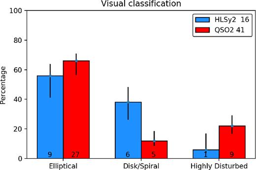
Results of the visual classification Method Vis-I (Section 3.1). The numbers within the bins in this and other histograms are the actual number of objects classified within each specific bin. The error bars in this and all histograms are 1σ Dirichlet multinomial distribution confidence intervals.
The main results are as follows:
Among QSO2s, 27/41 or 66%|$^{+5}_{-10}$| are visually classified as ellipticals, 5/41 or 12%|$^{+7}_{-4}$| are spirals or discs, and 9/41 or 22%|$^{+7}_{-6}$| are highly disturbed (HD) systems. Among HLSy2s, 9/16 or 56%|$^{+9}_{-15}$| are ellipticals, 6/16 or 38%|$^{+10}_{-12}$| are spirals or discs, and 1/16 or 6%|$^{+11}_{-3}$| is an HD system.
Thus, a minority of QSO2s are hosted by discs/spirals. This fraction is significantly higher in the HLSy2 sub-sample.
There is tentative evidence for the fraction of HD systems to be higher in QSO2s than in HLSy2s, although taking uncertainties into account the difference is not significant.
4.1.2 Methods Vis-II and Vis-III
The previous visual method does not allow the identification of all objects with signs of mergers/interactions, but only of the most morphologically disturbed systems. However, their identification can be done with the classification method Vis-II (see Section 3.1). The results are shown in Fig. 3 (see also Table 6, column 4).

The first result is that QSO2s and HLSy2s are distributed quite evenly among the four classes, from isolated objects, without (Class 0) or with (Class 0*) peculiar features, to objects with signatures of galaxy interactions at different stages (Classes 1 and 2). This means that powerful nuclear activity occurs both in isolated objects and at different phases of galactic interactions, as already found in different studies such as Ramos-Almeida et al. (2011) and Bessiere et al. (2012).
The additional classification of the peculiar features based on Ramos-Almeida et al. (2011) (Method Vis-III) provides complementary information: |$71{\%}^{+6}_{-8}$| of QSO2s show peculiar features that have been classified according to their aspect in column (5) of Table 6. For the HLSy2 sub-sample the percentage is |$56{\%}^{+12}_{-13}$|. These values may be lower limits, given the higher difficulty to identify peculiar features in galaxies with spiral/disc structures.
Bessiere et al. (2012) studied and classified the peculiar features in a complete sample of 20 SDSS QSO2s at 0.30 < |$z$| < 0.41 and with lO3 ≥ 8.5. Thirteen of these are also in our sample. They used deep Gemini Multi-Object Spectrograph-South optical broad-band images obtained with the r′-band filter (rG0326, λeff = 6300 Å, Δλ = 1360 Å). They found that ∼75 per cent of their QSO2s show evidence of peculiar features. If we focus on those objects in the HST sample with lO3 ≥ 8.5, we find the same rate as them: |$75{\%}^{+7}_{-11}$| show peculiar features.
Considering the 13 QSO2s that overlap with our study, Bessiere et al. (2012) confirm peculiar features in 11 objects. We confirm them in 10. The discrepant object is SDSS J011429.61+000036.7. They identify a second nucleus (which, given the unknown |$z$|, we have classified as projected companion ‘PC’) and a shell that is not clearly detected in the HST image.
4.2 Parametric classification
Following Section 3.2, we classify the host galaxies of our sample based on the dominant structural component identified as a result of the parametric fits. This method could not be applied to 15/57 objects, of which 14 are QSO2s and 1 is an HLSy2. In general, they present strongly distorted morphologies. These objects will be referred to as ‘highly disturbed’, in coherence with the visual classification. The results of the parametric method for individual objects are shown in Table 6. The distribution of the sample among the different classification groups is shown in Tables 7 and 8, and in Fig. 4 (left). The difference between these two tables is that Table 7 includes HD systems, while Table 8 does not.
![Left: results of the parametric classification for QSO2s and HLSy2s. ‘Bulge’ is bulge-dominated systems, which include galaxies with B/D > 1.2 and spheroidal systems (single Sérsic with n ≥ 2). ‘Disk’ is disc-dominated systems, which include galaxies with B/D < 0.8 and disc-like systems (single Sérsic with n < 2). ‘Bulge-Disk’ is systems for which 0.8 ≤ B/D ≤ 1.2 (zero found in the sample) and ‘PSF’ is systems where a point source contributes ≥50 per cent of the total light. The numbers within the bins and the error bars are explained in Fig. 2. Right: dependence of the galaxy classification with $L_ {\rm [O\,{\small III}]}$ (proxy of AGN power). For each luminosity bin, the number of galaxies classified within a certain class is indicated by the height of the corresponding coloured rectangle. For instance, in the the lO3 ∼ 8.25 bin there are three bulge-dominated and three disc-dominated galaxies. The vertical line corresponds to lO3 = 8.3, assumed as the dividing value between HLSy2s and QSO2s.](https://oup.silverchair-cdn.com/oup/backfile/Content_public/Journal/mnras/483/2/10.1093_mnras_sty2910/1/m_sty2910fig4.jpeg?Expires=1749948949&Signature=4Ju-TRE70W82v5zQw3ujbYZYfd6GlO7l9vJu8lE~VT4lXKzklWO4dLt~F6FI3TtmboUJl8PfmkUsp1Oa0Q8s37eNyqJTBfijdU1oc7SuavSY38ZmhgQ4xcXbg3hLv57f1gpAa7d084D3Kulj7RuFY~QAgDfmdbqED0ckAVWTEs0vlgJLG0JwkKkzL8lk1GRO6FRxlOA82FLvgWq3ZtCE5LAyhsWVB1fOXCb3wT30x7ymAuhXSXqvWiw~3SQu7IFkV7ktvQ2rZF-ffKgkeZm0DVUcqvBnK~tfSc5uPTta3gjN0JC3~OATCzuJk7Skk3x2LdtoM3rZUmjyDRJZpfUPJA__&Key-Pair-Id=APKAIE5G5CRDK6RD3PGA)
Left: results of the parametric classification for QSO2s and HLSy2s. ‘Bulge’ is bulge-dominated systems, which include galaxies with B/D > 1.2 and spheroidal systems (single Sérsic with n ≥ 2). ‘Disk’ is disc-dominated systems, which include galaxies with B/D < 0.8 and disc-like systems (single Sérsic with n < 2). ‘Bulge-Disk’ is systems for which 0.8 ≤ B/D ≤ 1.2 (zero found in the sample) and ‘PSF’ is systems where a point source contributes ≥50 per cent of the total light. The numbers within the bins and the error bars are explained in Fig. 2. Right: dependence of the galaxy classification with |$L_ {\rm [O\,{\small III}]}$| (proxy of AGN power). For each luminosity bin, the number of galaxies classified within a certain class is indicated by the height of the corresponding coloured rectangle. For instance, in the the lO3 ∼ 8.25 bin there are three bulge-dominated and three disc-dominated galaxies. The vertical line corresponds to lO3 = 8.3, assumed as the dividing value between HLSy2s and QSO2s.
The main results are as follows:
Bulge-dominated systems. This group includes spheroidal galaxies or galaxies with B/D > 1.2 (Section 3.2.4). It is the most numerous group both for QSO2s (18/41 or 44|${\%}^{+5}_{-10}$|) and for HLSy2s (10/16 or 63|${\%}^{+1}_{-21}$|). Taking uncertainties into account, no significant difference between QSO2s and HLSy2s is found.
If HD systems are excluded, no significant difference is found either (18/27 or 67%|$^{+4}_{-15}$| for QSO2s and HLSy2s (10/15 or 67%|$^{+3}_{-21}$|).
Disc-dominated systems: These are disc-like galaxies or galaxies with B/D < 0.8 (Section 3.2.4). Only 25%|$^{+8}_{-11}$|(4/16) of HLSy2 and 20%|$^{+6}_{-6}$| (7/41) of QSO2 galaxies are disc-dominated. The difference between both groups is not significant.
If HD systems are excluded, the fractions become 4/15 or 27%|$^{+10}_{-11}$| for HLSy2s and 8/27 or ∼29%|$^{+8}_{-9}$| for QSO2s.
Bulge + disc systems (B/D = 1.0 ± 0.2) have not been found (0%+9 of HLSy2s and 0%+3 of QSO2s).
Discs (not necessarily dominating the total galaxy flux) are identified in a significantly higher fraction of HLSy2s (7/16 or 44|${\%}^{+13}_{-11}$|) than QSO2s (10/41 or 24|${\%}^{+8}_{-6}$|).
If HD systems are excluded, the difference between both fractions disappears: HLSy2 (47%|$^{+13}_{-12}$|) and QSO2 (37%|$^{+10}_{-8}$|) have discs.
A point source component is isolated in a high fraction of objects: 29 (10 HLSy2s and 19 QSO2s) of the 42 (69%|$^{+7}_{-8}$|) for which the parametric analysis could be applied, with no significant difference between both groups. The relative contribution to the total flux varies between 3 per cent and 51 per cent, with average value 20.7 ± 2.9 per cent (median 14.2 per cent). The PSF dominates (≥50 per cent of the total flux) in just one HLSy2 and one QSO2.
4.3 Dependence of galaxy host with lO3
We have seen that, excluding highly disturbed systems, the parametric classification of the HLSy2 and QSO2 hosts are consistent within the errors.
We perform next a more detailed analysis of the dependence of galaxy properties with lO3, proxy for AGN power. For this, we use a finer sampling of the line luminosity range, instead of the coarse and somewhat arbitrary division in HLSy2 and QSO2 at threshold lO3 = 8.3. The results are shown in Fig. 4 (right).
A clear dependence of the galaxy properties on AGN power is revealed. While bulge-dominated systems spread across the total range of lO3, disc-dominated galaxies concentrate mostly at |$\mathrm{ lO}3\lesssim 8.6$|. This is in fact closer to the dividing luminosity lO3 = 8.5 between QSO2s and HLSy2s assumed by Zakamska et al. (2003) than to the 8.3 value assumed by Reyes et al. (2008). Considering the full sample, there are 10/36 or 28%|$^{+8}_{-6}$| disc-dominated galaxies below lO3 = 8.6 and 2/21 or 10%|$^{+10}_{-3}$| above.
The differentiation is even clearer when HD systems are excluded. 38%|$^{+10}_{-8}$| objects with lO3 < 8.6 are disc-dominated versus 13%|$^{+14}_{-5}$| above this luminosity. There are 56%|$^{+9}_{-10}$| bulge-dominated galaxies at lO3 < 8.6 and 87%|$^{+5}_{-14}$| at lO3 > 8.6.
The increasing incidence of bulge-dominated systems with AGN luminosity is also apparent when we study the variation with lO3 of the relative contribution of the spheroidal component to the total galaxy light (B/T) for the objects that could be fitted with galfit (Fig. 5). The average B/T increases with AGN power. Most objects with lO3 |$\gtrsim$| 8.6 have B/T |$\gtrsim$| 70 per cent, while at lower luminosities, the galaxies span the full range of possible B/T values.
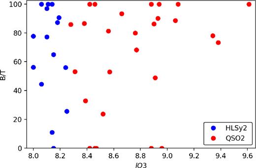
Relative contribution of the spheroidal component to the total galaxy light (B/T) versus lO3. Only galaxies that could be fitted with galfit are plotted. B/T increases with AGN power. For |$\mathrm{ lO}3\gtrsim$|8.6, most galaxies are bulge-dominated.
4.4 Contribution from a point source
A point source has been isolated in 29 of the 42 objects (69%|$^{+7}_{-8}$|) for which the parametric method could be applied. The relative contribution to the total light of the galaxy in this sub-sample is in the range light fraction (LF) ∼ 3–51 per cent with median value 14.2 per cent and standard deviation 14.8 per cent. Even when the LF is small (∼ a few per cent), this cannot be ignored in the fits, since the structural parameters of the hosts can be severely affected.
Our results are in good agreement with those of Inskip et al. (2010) (see Appendix B for a description of their sample). They found that the K-band images of 17 NLRGs are often contaminated by a point source. They identified this component in 12 objects with LF in the range ∼1–36 per cent and with median and standard deviation values 11.0 per cent and 10.9 per cent, respectively.
This unresolved component is a combination of different sources whose relative contribution changes with spectral range. While in Inskip et al. (2010) an enhanced contribution of the AGN direct light may play a role due to less severe extinction effects in the near-infrared, in our data the contamination by strong emission lines emitted by the compact narrow-line region (NLR) is possibly high in many objects (see Table 1). Compact continuum sources are also potential contributors such as nebular continuum associated with the NLR, scattered AGN light, and nuclear starbursts (Bruce et al. 2015; Dickson et al. 1995; Bessiere et al. 2017).
We have compared the galaxy host classification for objects with and without a point source (Table 4). The statistics is very poor and the errors large, so significant differences cannot be claimed. On the other hand, tentative evidence is hinted for a higher fraction of bulge-dominated systems among objects (both QSO2s and HLSy2s) with a point source.
Comparison between the galaxy classification of HLSy2s and QSO2s with and without a point source. The fractions are quoted in brackets. Tentative evidence is hinted for a higher fraction of bulge-dominated systems in objects without a point source.
| Parametric class | AGN type | With PS | Without PS |
|---|---|---|---|
| Bulge-dominated | HLSy2 | (6/10) 60%|$^{+4}_{-24}$| | (4/5) 80%|$^{+1}_{-35}$| |
| QSO2 | (11/19) 58%|$^{+5}_{-17}$| | (7/8) 88%|$^{+1}_{-28}$| | |
| Disc-dominated | HLSy2 | (3/10) 30%|$^{+10}_{-14}$| | (1/5) 20%|$^{+20}_{-10}$| |
| QSO2 | (7/19) 37%|$^{+12}_{-8}$| | (1/8) 13%|$^{+17}_{-6}$| | |
| PSF-dominated | HLSy2 | (1/10) 10%|$^{+14}_{-5}$| | N/A |
| QSO2 | (1/19) 5%|$^{+9}_{-2}$| | N/A |
List of the 42/57 objects that could be fitted with galfit and results of the best fits. C̠olumn (2): method to obtain the best fit. 1: Single Sérsic. 2A: Sérsic + disc, 2B: PS + Sérsic, 2C: PS + disc + Sérsic, 2D: other. Columns (3) and (4): total magnitude and effective radius Reff in kpc of the galfit galaxy model. Columns (5,6): magnitude and relative contribution (light fraction) to the total galaxy luminosity of the point source. Columns (7) to (12): magnitude, light fraction, and structural parameters of the first component identified with galfit. Columns (13) to (18): same for second component. Sérsic index n, axial ratio b/a, position angle (east of north) PA.
| Total | Point source | First profile component | Second profile component | ||||||||||||||
|---|---|---|---|---|---|---|---|---|---|---|---|---|---|---|---|---|---|
| cSDSS | Method | Mag | Reff | Mag | Light | Mag | Light | Reff | n | b/a | PA | Mag | Light | Reff | n | b/a | PA |
| name | galfit | (mag) | (kpc) | (mag) | fraction | (mag) | fraction | (kpc) | (º) | (mag) | fraction | (kpc) | (º) | ||||
| [1] | [2] | [3] | [4] | [5] | [6] | [7] | [8] | [9] | [10] | [11] | [12] | [13] | [14] | [15] | [16] | [17] | [18] |
| J005515.82−004648.6 | 2B | 19.3 | 1.5 | 20.4 | 35.00 | 19.7 | 65.00 | 2.4 | 1.2 | 0.57 | 68.5 | ||||||
| J011429.61+000036.7 | 2B | 17.5 | 5.9 | 21.3 | 6.70 | 18.2 | 93.30 | 13.0 | 4.0 | 0.74 | −58.7 | ||||||
| J011522.19+001518.5 | 1 | 18.1 | 4.5 | 18.1 | 100.00 | 6.3 | 4.0 | 0.59 | −52.8 | ||||||||
| J014237.49+144117.9 | 2B | 17.8 | 1.1 | 20.4 | 20.00 | 18.8 | 80.00 | 1.5 | 4.0 | 0.75 | −52.4 | ||||||
| J015911.66+143922.5 | 2B | 19.5 | 1.2 | 22.1 | 18.67 | 20.4 | 81.33 | 1.9 | 1.4 | 0.81 | −46.4 | ||||||
| J020234.56−093921.9 | 2A | 17.6 | 6.3 | 18.7 | 32.97 | 2.4 | 4.0 | 0.81 | −78.8 | 18.0 | 67.03 | 8.8 | 1.0 | 0.85 | −81.3 | ||
| J021059.66−011145.5 | 2B | 19.0 | 3.0 | 20.7 | 22.80 | 19.2 | 77.20 | 8.2 | 2.5 | 0.48 | 69.9 | ||||||
| J023411.77−074538.4 | 2D | 18.7 | 2.3 | 22.0 | 10.38 | 19.8 | 68.29 | 2.5 | 2.8 | 0.86 | 81.5 | 21.2 | 21.32 | 4.2 | 0.3 | 0.85 | 64.0 |
| J031946.03−001629.1 | 2D | 18.8 | 7.5 | 19.1 | 56.00 | 7.5 | 5.4 | 0.51 | −63.3 | 19.7 | 44.00 | 8.9 | 0.3 | 0.80 | −82.5 | ||
| J031927.22+000014.5 | 1 | 18.8 | 4.5 | 18.7 | 100.00 | 7.4 | 3.8 | 0.64 | 33.8 | ||||||||
| J032029.78+003153.5 | 2C | 17.0 | 12.8 | 21.6 | 2.99 | 19.3 | 23.71 | 3.4 | 4.0 | 0.85 | 63.9 | 17.8 | 73.3 | 28.9 | 1.0 | 0.51 | 72.7 |
| J034215.08+001010.6 | 1 | 19.2 | 1.1 | 19.1 | 100.00 | 0.7 | 6.0 | 0.82 | −14.7 | ||||||||
| J040152.38−053228.7 | 2B | 19.0 | 2.7 | 21.1 | 12.17 | 18.9 | 87.83 | 2.9 | 1.0 | 0.87 | −40.1 | ||||||
| J074811.44+395238.0 | 2B | 18.7 | 4.6 | 21.3 | 9.45 | 18.6 | 90.55 | 9.4 | 4.0 | 0.89 | −70.5 | ||||||
| J081125.81+073235.3 | 1 | 19.2 | 4.0 | 19.2 | 100.00 | 5.9 | 4.2 | 0.73 | −0.9 | ||||||||
| J082449.27+370355.7 | 2B | 19.0 | 1.3 | 21.1 | 14.20 | 19.1 | 85.80 | 2.0 | 5.7 | 0.72 | 62.5 | ||||||
| J082527.50+202543.4 | 2B | 19.7 | 1.1 | 20.4 | 49.48 | 20.4 | 50.52 | 1.5 | 1.0 | 0.95 | −64.5 | ||||||
| J083028.14+202015.7 | 2C | 18.5 | 2.5 | 20.8 | 11.85 | 19.2 | 48.83 | 1.8 | 4.0 | 0.33 | −38.6 | 19.4 | 39.32 | 3.1 | 1.0 | 0.95 | 11.2 |
| J084041.08+383819.8 | 2C | 17.8 | 7.1 | 20.8 | 6.46 | 19.7 | 18.47 | 4.2 | 0.4 | 0.33 | 5.2 | 18.1 | 75.08 | 9.5 | 1.0 | 0.81 | −28.3 |
| J084309.86+294404.7 | 2B | 18.7 | 3.1 | 20.3 | 22.02 | 19.0 | 77.98 | 6.7 | 2.6 | 0.87 | −49.0 | ||||||
| J084856.58+013647.8 | 1 | 17.1 | 4.9 | 17.9 | 100.00 | 18.7 | 5.0 | 0.87 | −39.6 | ||||||||
| J084943.82+015058.2 | 2C | 19.5 | 2.2 | 21.2 | 21.57 | 20.2 | 44.41 | 3.8 | 4.0 | 0.41 | 66.4 | 20.7 | 34.03 | 3.1 | 1.0 | 0.47 | 50.8 |
| J090414.10−002144.9 | 2B | 17.8 | 2.9 | 21.3 | 9.90 | 18.3 | 90.10 | 9.6 | 6.5 | 0.52 | −67.3 | ||||||
| J092318.06+010144.8 | 1 | 18.8 | 3.1 | 18.8 | 100.00 | 4.1 | 4.0 | 0.68 | −46.5 | ||||||||
| J094209.00+570019.7 | 2D | 18.7 | 1.6 | 19.9 | 31.42 | 19.4 | 53.12 | 4.3 | 5.2 | 0.91 | −54.4 | 20.7 | 15.46 | 4.3 | 0.2 | 0.75 | −86.3 |
| J094350.92+610255.9 | 2B | 19.6 | 1.0 | 20.2 | 49.77 | 20.3 | 50.23 | 1.4 | 1.0 | 0.85 | −48.1 | ||||||
| J095629.06+573508.9 | 2B | 19.0 | 3.2 | 21.3 | 13.44 | 19.1 | 86.56 | 4.5 | 2.2 | 0.58 | −80.5 | ||||||
| J100329.86+511630.7 | 1 | 18.4 | 4.8 | 18.4 | 100.00 | 6.3 | 2.5 | 0.48 | 75.8 | ||||||||
| J103639.39+640924.7 | 1 | 17.8 | 7.3 | 17.8 | 100.00 | 14.0 | 4.0 | 0.65 | 19.6 | ||||||||
| J112907.09+575605.4 | 2D | 19.1 | 2.4 | 21.8 | 9.38 | 19.2 | 73.34 | 5.1 | 4.0 | 0.70 | −5.2 | 21.0 | 17.28 | 1.8 | 0.2 | 0.07 | −7.6 |
| J113710.78+573158.7 | 1 | 18.6 | 3.3 | 18.6 | 100.00 | 7.5 | 6.5 | 0.53 | −48.3 | ||||||||
| J140740.06+021748.3 | 2D | 19.2 | 1.5 | 19.3 | 86.28 | 1.2 | 5.6 | 0.46 | −45.3 | 21.2 | 13.72 | 5.2 | 0.5 | 0.15 | −35.8 | ||
| J150117.96+545518.3 | 2B | 17.2 | 6.1 | 19.5 | 11.39 | 17.2 | 88.61 | 8.5 | 2.3 | 0.88 | 62.3 | ||||||
| J154133.19+521200.1 | 2A | 18.0 | 6.7 | 19.5 | 25.59 | 2.0 | 4.6 | 0.65 | −29.7 | 18.1 | 74.41 | 9.8 | 1.0 | 0.79 | −19.7 | ||
| J154613.27−000513.5 | 2B | 19.0 | 3.8 | 21.3 | 12.71 | 19.1 | 87.29 | 5.9 | 2.4 | 0.84 | −51.2 | ||||||
| J172419.89+551058.8 | 2B | 19.3 | 1.4 | 20.3 | 43.86 | 19.9 | 56.14 | 5.0 | 1.7 | 0.63 | 63.9 | ||||||
| J172603.09+602115.7 | 2B | 19.8 | 1.2 | 20.6 | 47.06 | 20.3 | 52.94 | 2.6 | 1.4 | 0.52 | 45.4 | ||||||
| J173938.64+544208.6 | 2C | 19.2 | 2.6 | 20.9 | 20.51 | 20.3 | 35.77 | 1.9 | 0.8 | 0.54 | 37.9 | 20.1 | 43.72 | 8.5 | 1.0 | 0.51 | 33.4 |
| J214415.61+125503.0 | 2C | 18.5 | 1.2 | 19.0 | 50.67 | 19.8 | 11.05 | 16.6 | 5.4 | 0.32 | −32.9 | 19.2 | 38.29 | 5.1 | 1.0 | 0.73 | −72.2 |
| J223959.04+005138.3 | 2C | 18.9 | 3.6 | 20.5 | 22.12 | 20.7 | 19.38 | 2.1 | 0.3 | 0.74 | −1.8 | 19.2 | 58.50 | 9.3 | 1.0 | 0.50 | 61.8 |
| J231755.35+145349.4 | 2B | 18.3 | 6.2 | 22.1 | 3.10 | 18.3 | 96.90 | 9.7 | 2.0 | 0.60 | 79.1 | ||||||
| J231845.12−002951.4 | 2D | 18.4 | 4.3 | 20.1 | 9.85 | 18.1 | 77.73 | 24.7 | 4.8 | 0.78 | 48.6 | 20.6 | 12.41 | 7.2 | 0.3 | 0.20 | 23.4 |
Results of the visual and parametric classification (see Section 3 for details). Column (3) indicates the galaxy morphological type based on Method Vis-I: El (elliptical), Sp (spiral), disc (disc galaxy with no obvious spiral arms), HD (highly disturbed: when 2 or more components are interacting and make the classification in the previous groups difficult). Column (4): type of merger based on Method Vis-II following Rodríguez Zaurín et al. (2011) and Veilleux et al. (2002): 0 = Isolated undisturbed galaxy, 0* = Isolated disturbed galaxy, 1 = two nuclei with projected separation > 1.5 kpc, 2 = two nuclei with projected separation ≤1.5 or single nucleus with signatures of a post-coalescence phase. Column (5) specifies the nature of the peculiar features based on Method Vis-III following Ramos-Almeida et al. (2011). T: tidal tail; F: fan; B: bridge; S: shell; D: dust feature; 2N: double nucleus; A: amorphous halo; I: irregular feature; IC: interacting companion. Other features we include in this work are 2N*: two nuclei with relative distance greater than 1.5 kpc; PC: projected companion, that is, there is an object close to the target in projection with no clear physical relation; K: knot; tt: streams. A question mark ‘?’ indicates uncertain classification or identification. Column (6): classification based on the parametric method (Table 5). N/A refers to objects that could not be fitted with galfit. Column (7): type of profile according to the dominant structural component: ‘HD’ in this column is for highly disturbed objects that could not be fitted with galfit. The vast majority are highly disturbed systems. Point source: a system dominated by a spatially unresolved source; disc-dominated: a system dominated by a disc or disc-like component; bulge-dominated: a system dominated by a spheroidal component. Column (8): comparison between the visual and parametric classifications.
| This work | B/T classification | Visual versus parametric | |||||
|---|---|---|---|---|---|---|---|
| Object SDSS | lO3 | Vis-I | Vis-II | Vis-III | Method | Details | |
| [1] | [2] | [3] | [4] | [5] | [6] | [7] | [8] |
| J002531.46−104022.2 | 8.73 | HD | 1 | 2N, T, K? | N/A | HD | |
| J005515.82−004648.6 | 8.15 | El | 0 | 2B | Disc-dominated | El versus disc-dominated | |
| J011429.61+000036.7 | 8.66 | El | 0 | PC | 2B | Bulge-dominated | |
| J011522.19+001518.5 | 8.14 | El | 0* | A, tt, PC | 1 | Bulge-dominated | |
| J014237.49+144117.9 | 8.76 | El | 0* | PC, S,D, tt, K? | 2B | Bulge-dominated | |
| J015911.66+143922.5 | 8.56 | El | 0 | 2B | Disc-dominated | El versus disc-dominated | |
| J020234.56−093921.9 | 8.39 | Sp | 1 | IC,B, K? | 2A | Disc-dominated | |
| J021059.66−011145.5 | 8.10 | Sp | 0* | S | 2B | Bulge-dominated | Sp versus bulge-dominated |
| J021758.18−001302.7 | 8.55 | HD | 2 | T,D | N/A | HD | |
| J021834.42−004610.3 | 8.85 | HD | 1 | T,C,IC = 2N | N/A | HD | |
| J022701.23+010712.3 | 8.90 | HD | 2 | 2 N, T, D, S, A | N/A | HD | |
| J023411.77−074538.4 | 8.77 | El | 0 | 2D | Bulge-dominated | ||
| J031946.03−001629.1 | 8.24 | Sp or Disc | 0 | 2D | Bulge-dominated | Sp or disc versus bulge-dominated | |
| J031927.22+000014.5 | 8.06 | El | 0* | F, tt? | 1 | Bulge-dominated | |
| J032029.78+003153.5 | 8.52 | El | 0* | D, PC | 2C | Disc-dominated | El versus disc-dominated |
| J032533.33−003216.5 | 9.06 | El | 2 | T | N/A | HD | El versus HD |
| J033310.10+000849.1 | 8.13 | HD | 1 | 2N/D?, T, K?, IC | N/A | HD | |
| J034215.08+001010.6 | 9.08 | El | 0 | 1 | Bulge-dominated | ||
| J040152.38−053228.7 | 8.96 | El | 0* | A, PC? | 2B | Disc-dominated | El versus disc-dominated |
| J074811.44+395238.0 | 8.19 | El | 2 | T, K? | 2B | Bulge-dominated | |
| J081125.81+073235.3 | 8.88 | El | 0* | A, IC?, I | 1 | Bulge-dominated | |
| J081330.42+320506.0 | 8.83 | El? | 2 | T,tt, D, I, A | N/A | HD | El? versus HD |
| J082449.27+370355.7 | 8.28 | El | 0 | 2B | Bulge-dominated | ||
| J082527.50+202543.4 | 8.88 | El | 0 | 2B | Disc-dominated | El versus disc-dominated | |
| J083028.14+202015.7 | 8.91 | El | 0 | 2C | Bulge-dominated | ||
| J084041.08+383819.8 | 8.47 | Sp | 2 | T, K? | 2C | Disc-dominated | |
| J084309.86+294404.7 | 9.34 | El | 0 | 2B | Bulge-dominated | ||
| J084856.58+013647.8 | 8.46 | El | 0* | S, A, PC | 1 | Bulge-dominated | |
| J084943.82+015058.2 | 8.06 | El | 0 | 2C | Bulge-dominated | ||
| J090307.84+021152.2 | 8.42 | HD | 1/2 | 2N*, T, K, D | N/A | HD | |
| J090414.10−002144.9 | 8.93 | El | 2 | T, F | 2B | Bulge-dominated | |
| J090801.32+434722.6 | 8.31 | El | 2 | T, I, K | N/A | HD | El versus HD |
| J092318.06+010144.8 | 8.94 | Sp | 0* | T? | 1 | Bulge-dominated | Sp versus B |
| J092356.44+012002.1 | 8.59 | El | 1/2 | T | N/A | HD | El versus HD |
| J094209.00+570019.7 | 8.31 | El | 1 | T, D, F, tt, PC | 2D | Bulge-dominated | |
| J094350.92+610255.9 | 8.46 | El | 0 | 2B | Point source | El versus point source | |
| J095629.06+573508.9 | 8.38 | El | 0 | 2B | Bulge-dominated | ||
| J100329.86+511630.7 | 8.11 | El | 2 | T, A, F | 1 | Bulge-dominated | |
| J103639.39+640924.7 | 8.42 | El | 2 | T, PC | 1 | Bulge-dominated | |
| J112907.09+575605.4 | 9.38 | El | 0* | I | 2D | Bulge-dominated | |
| J113710.78+573158.7 | 9.61 | El | 0* | T, tt | 1 | Bulge-dominated | |
| J133735.01−012815.7 | 8.72 | El | 2 | T?, 2N, I | N/A | HD | El versus HD |
| J140740.06+021748.3 | 8.90 | Sp or Disc | 0 | 2D | Bulge-dominated | Sp or disc versus bulge-dominated | |
| J143027.66−0056149 | 8.44 | HD | 1 | 2N, T, IC?, K, A | N/A | HD | |
| J144711.29+021136.2 | 8.45 | HD | 1/2 | 2N*, T, B | N/A | HD | |
| J150117.96+545518.3 | 9.06 | El? | 1 | IC, S,D, T, B, K? | 2B | Bulge-dominated | |
| J154133.19+521200.1 | 8.25 | Sp | 2 | S, K, T, IC? | 2A | Disc-dominated | |
| J154337.81−004420.0 | 8.40 | HD | 1 | 2N, T,F,I, A | N/A | HD | |
| J154613.27−000513.5 | 8.18 | El | 0 | 2B | Bulge-dominated | ||
| J172419.89+551058.8 | 8.00 | El | 0 | 2B | Disc-dominated | El versus D | |
| J172603.09+602115.7 | 8.57 | El | 0 | 2B | Disc-dominated | El versus disc-dominated | |
| J173938.64+544208.6 | 8.42 | Sp or Disc | 0* | tt? | 2C | Disc-dominated | |
| J214415.61+125503.0 | 8.14 | El | 2 | I,T | 2C | Point source | El versus point dource |
| J215731.40+003757.1 | 8.39 | HD | 1 | D,IC | N/A | HD | |
| J223959.04+005138.3 | 8.15 | Sp or Disc | 0* | A? | 2C | Disc-dominated | |
| J231755.35+145349.4 | 8.10 | Sp | 0 | C | 2B | Bulge-dominated | Sp versus bulge-dominated |
| J231845.12−002951.4 | 8.00 | Sp | 0 | 2D | Bulge-dominated | Sp versus bulge-dominated | |
We cannot discard that this is an artificial effect. We may be missing a point source in some objects where this contribution cannot be clearly recognized by our fitting method. Ignoring the point souce would result in steeper Sérsic profiles (and, thus, higher n values) for the central region of the galaxy hosts, so some may be misclassified as bulge-dominated as a consequence. If this is the case, the fraction of bulge-dominated systems in galaxies with no point source would represent an upper limit.
The other alternative is that there is a real intrinsic difference between both groups (with and without point source contribution). Understanding the physical origin of such a difference, if confirmed, would be of great interest, possibly pointing to differences in the opening angle of the central obscuring structure and/or the amount of obscuring dust in the central regions and/or orientation.
4.5 Kormendy relation
We show in Fig. 6 the Kormendy relation for our sample of host galaxies (Hamabe & Kormendy 1987). The effective radius, re, and the surface brightness magnitude at re, μ(re), are plotted only for the spheroidal component of galaxies. Errors on re are expected to be typically ∼10 per cent (Buitrago, Ferreras & Kelvin 2018). We have assumed Δμe = 0.5 magnitude errors on μ(re). This is based on the study of how μe varies for a 10 per cent change in re using different Sérsic profiles. This variation, Δμe, is clearly larger in steeper (high-n) profiles and it can be up to ∼0.5 mag. This is the error we have used, which is therefore conservative.
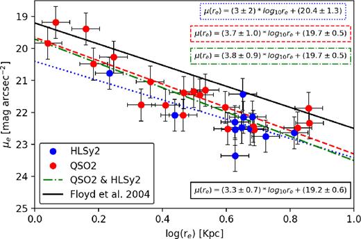
Relation between surface magnitude and effective radius for the spheroidal galaxies and bulges in our sample of luminous AGNs. The best fits are shown for the QSO2s, the HLSy2s, and both groups together. The slope is consistent with that found by Floyd et al. (2004) for the bulge-dominated hosts of a sample of 14 QSO1s at |$z$| ∼ 0.4.
The three trends have correlation coefficients ρ2 =0.46, 0.76, and 0.71, respectively [the weak trend for HLSy2s is biased by the outlying measurement of the more compact system with log(re)∼0.2 kpc].
These relations are consistent within the errors with the scaling relation found by Bernardi et al. (2003) for 9000 SDSS early-type galaxies at 0.01 ≤ |$z$| ≤ 0.3 (slope 3.33 ± 0.09).
Our sample is shifted down the vertical axis by ∼0.6 magnitudes with respect to Floyd et al. (2004) QSO1s, although the two samples are within the scatter both have (Δμe ∼ ±0.6). Both samples are basically at identical |$z$|, and thus redshift dimming does not play a role. We do not believe it is a consequence of the filters used either: 10 of 17 objects of Floyd et al. (2004) were observed with the same filter F814W as the majority of our sample. The other 7 were observed with the F791W filter, redder and slightly narrower. Several objects in our sample were observed with the ACS and with a significantly narrower filter than F814W. These objects are not shifted in any sense relative to the rest of the objects. The filters, therefore, do not seem to have any influence. Another possible effect is that Floyd et al. (2004) plot μe and re of the galaxies, and not only the spheroids, as we have done. Although all are bulge-dominated, not removing the contribution of a disc may result in brighter magnitudes. A final possibility is that the QSO1s are hosted by more luminous and more massive spheroids (see below).
The average 〈re〉 of the spheroidal component is 3.4 ± 0.5 kpc (median 3.0 ± 1.2 kpc) and 4.3 ± 0.4 kpc (median 4.5 ± 0.3 kpc) for the QSO2s and the HLSy2s, respectively. For comparison, Greene et al. (2009) obtain 〈re〉 = 3.1 ± 0.8 kpc (median 2.6 ± 0.5 kpc) for their sample of luminous QSO2s (Appendix B).3 These results tentatively suggest that QSO2s may be hosted by smaller spheroids than HLSy2s. The uncertainties due to the poor statistics are however too large to confirm this.
We have also measured re for the total galaxies (spheroidal + disc components when present), excluding the point source, which can result in an underestimation of re even when the flux contribution is low (<10 per cent).4 We obtain 〈re〉 = 3.9 ± 0.6 kpc (median 3.3 ± 1.6 kpc) for the QSO2s and 5.0 ± 1.5 kpc (median 4.8 ± 0.9 kpc) for the HLSy2s.
The QSO2 sizes are significantly smaller than those measured for QSO1s and NLRGs at similar |$z$| by other authors.5 The Inskip et al. (2010) sample of NLRGs have 〈re〉 = 10.1 ± 1.6 kpc (median 10.0 kpc). Dunlop et al. (2003) radio-quiet and radio-loud QSO1s have 〈re〉 = 7.6 ± 1.2 kpc (median 6.4 kpc) and 〈re〉 = 8.2 ± 0.8 kpc (median 8.0 kpc), respectively. Floyd et al. (2004) obtain 〈re〉 = 7.2 ± 1.3 kpc and 6.1 ± 1.3 kpc for radio-loud and radio-quiet QSO1s, respectively. Finally, 〈re〉 = 7.7 ± 3.6 kpc for the Falomo et al. (2014) QSO1 sample.
Shen et al. (2003) found that early-type galaxies (n > 2.5) at |$z$| ∼ 0 with log(M*/M⊙) in the range 10.0–11.0 have re ∼2.1–4.2 kpc. Only galaxies with log(|$M_{\rm *})\gtrsim$|11.4 have sizes >7 kpc. Wylezalek et al. (2016) inferred log(M*/M⊙) = 9.8–11.0 for a sample of 20 QSO2s at similar |$z$| as our sample, with median and average values 10.4 and 10.5, respectively.6
Therefore, the 〈re〉 we obtain for our QSO2s are in reasonable agreement with those expected based on the typical stellar masses inferred for other luminous QSO2s. It is possible that the QSO1 and NLRG samples mentioned above are hosted by more massive galaxies.
5 DISCUSSION
Studies of low-|$z$| QSO1s (|$z\lesssim$| 0.5) since the era of HST show that luminous quasars (radio-loud and radio-quiet) are hosted by a diversity of host galaxies, including ellipticals as bright as the brightest cluster ellipticals, normal ellipticals, spirals, and highly disturbed interacting systems (e.g. Bahcall et al. 1997; Kukula et al. 2001; Percival et al. 2001; Dunlop et al. 2003; Floyd et al. 2004; Falomo et al. 2014).
Some of these works have suggested that the type of galaxy host depends on AGN power, so the most luminous AGNs (quasars) tend to be hosted by massive ellipticals (Dunlop et al. 2003; Floyd et al. 2004). This is however controversial and other works claim a higher incidence of galaxies with discs in luminous quasars (e.g. Cales et al. 2011; Falomo et al. 2014).
The contribution of this work to the topic of the host galaxies associated with quasars is based on the fact that (1) due to their recent discovery, just a few studies exist (two, to the best of our knowledge: Greene et al. 2009; Wylezalek et al. 2016) regarding the structural properties of |$z$| < 1 QSO2 host galaxies . They have been focused on samples of up to ∼20 objects. We expand these works with 41 more QSO2s and complement them with 16 HLSy2s. (2) We take into account factors that sometimes have not been considered, such as the high incidence of highly disturbed systems, the contribution of a point source and/or the presence of several structural components in galaxies. (3) We perform a thorough comparative study with related parametric works of the host galaxies of luminous AGNs at similar |$z$| (see Section 5.1).
Our analysis has shown a wide diversity of galaxy hosts among both HLSy2s and QSO2s (Tables 7 and 8). An interesting result is that a high fraction (∼55 per cent) of QSO2s are not hosted by bulge-dominated galaxies. Although these are the most numerous group (44|${\%}^{+5}_{-10}$|), more than half QSO2s are hosted by other galaxy types, mostly highly disturbed systems due to galaxy interactions (34|${\%}^{+6}_{-9}$|) and disc-dominated systems (20|${\%}^{+6}_{-6}$|). The main difference between QSO2s and HLSy2s is the lower incidence of morphologically disturbed systems among HLSy2s (6|${\%}^{+10}_{-3}$|). This is consistent with a scenario in which galaxy interactions are the dominant mechanism triggering the activity at the highest AGN power (e.g. Hopkins et al. 2008; Ramos-Almeida et al. 2011; Bessiere et al. 2012).
Comparison with other works. B/D includes intermediate classification in works that use only one Sérsic profile and n has an intermediate value between disc-dominated and bulge-dominated objects assumed by the authors.
| Disc-dominated | Bulge-dominated | B + D | Point source | Disturbed | |
|---|---|---|---|---|---|
| This work (HLSy2) | |$25\%^{+8}_{-11}$| | |$63\%^{+1}_{-21}$| | 0%+9 | |$6\%^{+10}_{-3}$| | |$6\%^{+10}_{-3}$| |
| This work (QSO2) | |$20\%^{+6}_{-6}$| | |$44\%^{+5}_{-10}$| | 0%+4 | |$2\%^{+5}_{-0.9}$| | |$34\%^{+6}_{-9}$| |
| Dunlop et al. (2003) (RL-QSO1) | 100%−16 | ||||
| Dunlop et al. (2003) (RQ-QSO1) | |$15\%^{+15}_{-6}$| | |$85\%^{+6}_{-15}$| | |||
| Floyd et al. (2004) (QSO1) | |$18\%^{+11}_{-7}$| | |$76\%^{+8}_{-13}$| | |$6\%^{+11}_{-3}$| | ||
| Falomo et al. (2014) (QSO1) | |$42\%^{+3}_{-3}$| | |$37\%^{+3}_{-3}$| | |$21\%^{+3}_{-3}$| | ||
| Cales et al. (2011) (QSO1) | |$21\%^{+8}_{-7}$| | |$62\%^{+4}_{-14}$| | |$3\%^{+7}_{-1.2}$| | |$14\%^{+8}_{-5}$| | |
| Greene et al. (2009) (QSO2) | |$20\%^{+12}_{-8}$| | |$53\%^{+9}_{-16}$| | |$27\%^{+12}_{-10}$| | ||
| Wylezalek et al. (2016) (QSO2) | |$10\%^{+11}_{-4}$| | |$90\%^{+4}_{-11}$| | |||
| Inskip et al. (2010) (NLRG) | |$6\%^{+11}_{-3}$| | |$88\%^{+1}_{-17}$| | |$6\%^{+11}_{-3}$| |
As Table 7 but excluding highly disturbed systems.
| Disc-dominated | Bulge-dominated | B + D | |
|---|---|---|---|
| This work (HLSy2) | |$29\%^{+12}_{-10}$| | |$71\%^{+5}_{-19}$| | 0%+11 |
| This work (QSO2) | |$31\%^{+9}_{-9}$| | |$69\%^{+6}_{-13}$| | 0%+7 |
| Dunlop et al. (2003) (RL-QSO1) | 100%−16 | ||
| Dunlop et al. (2003) (RQ-QSO1) | |$15\%^{+15}_{-6}$| | |$85\%^{+6}_{-15}$| | |
| Floyd et al. (2004) (QSO1) | |$18\%^{+11}_{-7}$| | |$76\%^{+8}_{-13}$| | |$6\%^{+11}_{-3}$| |
| Falomo et al. (2014) (QSO1) | |$42\%^{+3}_{-3}$| | |$37\%^{+3}_{-3}$| | |$21\%^{+3}_{-3}$| |
| Cales et al. (2011) (QSO1) | |$24\%^{+9}_{-7}$| | |$72\%^{+5}_{-13}$| | |$4\%^{+8}_{-1.4}$| |
| Greene et al. (2009) (QSO2) | |$27\%^{+19}_{-9}$| | |$73\%^{+9}_{-17}$| | |
| Wylezalek et al. (2016) (QSO2) | |$10\%^{+11}_{-4}$| | |$90\%^{+4}_{-11}$| | |
| Inskip et al. (2010) (NLRG) | |$6\%^{+11}_{-3}$| | |$88\%^{+1}_{-17}$| | |$6\%^{+11}_{-3}$| |
Although discs are identified in 44|${\%}^{+13}_{-11}$| of HLSy2s and 24|${\%}^{+8}_{-6}$| of QSO2s, disc-dominated systems represent a minority (25|${\%}^{+8}_{-11}$| of HLSy2s and 20|${\%}^{+6}_{-6}$| of QSO2s). Excluding highly disturbed systems, if we consider the coarse division QSO2 versus HLSy2 at lO3 = 8.3, both groups show a similar distribution among galaxy types (Tables 7 and 8). However, a more careful analysis reveals that the galaxy properties do change with AGN power: The relative contribution of the spheroidal component to the total galaxy light (B/T) increases with lO3 (Section 4.3). Excluding the complex merger/interaction systems, B/T |$\gtrsim$| 0.7 for most galaxies with |$\mathrm{ lO}3\,\gtrsim$| 8.6. As other authors have argued, this is naturally expected if more powerful AGNs are powered by more massive black holes which in turn are hosted by more massive bulges or spheroids (Magorrian et al. 1998; Dunlop et al. 2003). Constraining the galaxy masses of the sample studied here would be very valuable to investigate this scenario.
5.1 Comparison with other works
We put the results of our parametric analysis in the context of other relevant works. We focus our comparison on the QSO2 sub-sample and related studies of AGNs with quasar-like luminosities (QSO1s, QSO2s, and NLRGs). While our HLSy2s are at the high end of Sy2 luminosities, related studies on Seyferts cover a much wider range usually extending to significantly lower AGN power, so the comparison is not trivial (Kauffmann et al. 2003).
We also focus on studies based on samples at |$z\lesssim$| 0.5. The comparison with high-|$z$| studies is complicated by the limited physical spatial information and/or the shallowness of the data and/or the different rest-frame spectral range (e.g. rest-frame ultraviolet at |$z$| > 2 versus rest-frame optical at low |$z$|). Detailed information on all referenced works can be found in Appendix B.
Firm conclusions regarding the origin of some discrepancies and similarities between works are not possible due to the numerous potential influencing factors on the galaxy classification: poor statistics, data properties (depth, spectral range, spatial resolution), sample selection (range of AGN luminosities, radio-loudness, obscured versus unobscured), fitting method (e.g. one versus several structural components; classification criteria based on n values). For the sake of clarity, we mention for each work the available information that can help the reader identify the possible influencing factors (Appendix B). The results of all works are summarized in Tables 7 and 8. The confidence intervals have been calculated as in Section 4.1.1.
In spite of the above limitations, some interesting results appear, which can be summarized as follows.
A clear difference between works is the incidence of highly disturbed merger/interaction systems, which are absent in several works while they account for ∼34 per cent of our QSO2 sample. The reason for the discrepancy lies, at least in part, in that the classification and/or fitting methods are often not sensitive to the distinction of such systems.
In general, all works are consistent regarding the fraction of disc-dominated galaxies (∼10-20 per cent) and B + D systems (|$\lesssim$| a few per cent) in radio-quiet quasars. This fraction is tentatively lower in radio-loud QSO1s and NLRGs (|$\lesssim$|6 per cent; Dunlop et al. 2003; Inskip et al. 2010). This is consistent with the fact that powerful radio-loud objects tend to be hosted by massive elliptical galaxies (Matthews, Morgan & Schmidt 1964; Best et al. 2005).
Falomo et al. (2014) are an exception. They find a significantly higher fraction of disc-dominated systems (42%|$^{+3}_{-3}$|) and B + D (21%|$^{+3}_{-3}$|). They identify discs in a high fraction of quasars ∼63 per cent (e.g. ∼24 per cent in our sample). A real difference in the type of galaxy hosts cannot be discarded, but it must be kept in mind that the fitting and classification method applied are, as the authors warn, too simplistic and can only yield a preliminary indication of the morphology (Appendix B).
All works are consistent in that the most numerous group of host galaxies are always bulge-dominated (Falomo et al. 2014 are again an exception). On the other hand, the percentage varies significantly. In general, studies that do not separate complex merger/interaction systems (Dunlop et al. 2003; Floyd et al. 2004; Inskip et al. 2010; Wylezalek et al. 2016) result in a higher fraction of bulge-dominated galaxies (∼76–100 per cent) compared with other works where disturbed systems are identified (44–62 per cent; our work; Greene et al. 2009; Cales et al. 2011). Thus, the classification criteria may play a role in the observed differences.
Moreover, intrinsic differences between samples probably also play a role. For instance, the radio-loud (Dunlop et al. 2003; Inskip et al. 2010) and most luminous samples (Wylezalek et al. 2016) show tentative evidence of the highest fraction of bulge-dominated systems. This is naturally expected. On one hand, radio loudness is favoured in massive bulge-dominated galaxies, as mentioned above. On the other hand, as we have seen, the relative contribution of the spheroidal component to the total galaxy light increases with lO3, a proxy of AGN power (Section 4.3).
6 SUMMARY AND CONCLUSIONS
We have studied the morphological and parametric properties of the host galaxies of 57 optically selected luminous type 2 AGNs at |$0.3 \lesssim z \lesssim 0.4$| from the SDSS. The sample consists of 41 QSO2s with 8.31 ≤ lO3 ≤ 9.61 and 16 HLSy2s with 8.06 ≤ lO3 ≤ 8.28. Our study is based on HLA archive ACS/WFC and WFPC2 HST images. Both samples contain ∼44 per cent of all SDSS optically selected QSO2s and HLSy2s within the same |$z$| and |$L_{\rm [O\,{\small III}]}$| ranges. Although uncertainties remain regarding the exact selection criteria, we consider them an adequate representation of the original total SDSS samples.
Due to the recent discovery of QSO2s in large numbers, the structural properties of their host galaxies are poorly known. To our knowledge, only two related studies have been published for |$z$| <1 QSO2s, with 35 QSO2 hosts parametrized so far (Greene et al. 2009; Wylezalek et al. 2016). Our work expands this investigation with 41 more QSO2s and complements it with 16 HLSy2s.
We have classified the galaxies both visually and, most importantly, parametrically using the code galfit. The parametric analysis is essential to isolate and parametrize the individual structural galactic components and, ultimately, classify the galaxies in terms of the dominant component.
The main results and conclusions of our study are as follows:
There is a wide diversity of galaxy hosts among both HLSy2s and QSO2s. Less than half (44|${\%}^{+5}_{-10}$|) QSO2s are hosted by bulge-dominated galaxies (in our terminology this includes spheroidal galaxies and galaxies with B/D > 1.2). More than half are hosted by other galaxy types, mostly highly disturbed systems due to galaxy mergers/interactions (34|${\%}^{+6}_{-9}$|) and disc-dominated systems (20|${\%}^{+6}_{-6}$|; these are disc-like galaxies and galaxies with B/D < 0.8). A minority of galaxies are dominated by a point source (2|${\%}^{+5}_{-0.9}$|).
Among HLSy2s, 63|${\%}^{+1}_{-21}$| are bulge-dominated, 25|${\%}^{+8}_{-11}$| are disc-dominated, and 6|${\%}^{+10}_{-3}$| are highly disturbed systems; 6|${\%}^{+10}_{-3}$| are dominated by a point source.
A significant difference between QSO2s and HLSy2s is the higher incidence of morphologically disturbed systems among QSO2s (34|${\%}^{+6}_{-9}$| versus 6|${\%}^{+10}_{-3}$|). This is consistent with a scenario in which galaxy interactions are the dominant mechanism triggering the activity at the highest AGN power.
Discs are identified in a significantly higher fraction of HLSy2s (44|${\%}^{+13}_{-11}$|) than QSO2s (24|${\%}^{+8}_{-6}$|) but this is a result of the lower fraction of disturbed systems among Seyferts. When these are not considered, the fractions become consistent within the errors (47|${\%}^{+13}_{-12}$| HLSy2s and 37|${\%}^{+10}_{-8}$| QSO2s).
The coarse and somewhat arbitrary division between HLSy2s and QSO2s at lO3 = 8.3 is not adequate to unveil trends of galaxy host with lO3 (used here as proxy of AGN power). A more detailed analysis using a finer sampling of lO3 reveals a clear dependence of the galaxy properties on AGN power. The relative contribution of the spheroidal component to the total galaxy light (B/T) increases with |$L_ {\rm [O\,{\small III}]}$|. B/T |$\gtrsim$| 0.7 for most QSO2s with |$\mathrm{ lO}3\gtrsim$|8.6, while at lower luminosities the galaxies span the full range B/T ∼ 0.0–1.0. While bulge-dominated systems spread across the total range of |$L_ {\rm [O\,{\small III}]}$| of the sample, most disc-dominated galaxies concentrate at lO3 |$\lesssim$| 8.6.
As other authors have argued, this is naturally expected if more powerful AGNs are powered by more massive black holes which in turn are hosted by more massive bulges or spheroids. Constraining the galaxy masses of the sample studied here would be very valuable to investigate this scenario.
A point source component is isolated in a high fraction of objects (10/16 or |$63{\%}^{+11}_{-13}$| of HLSy2s and 19/41 or |${\sim }46{\%}^{+8}_{-8}$| of QSO2s), although it rarely dominates the total flux. The relative contribution to the total galaxy light is in the range ∼3–51 per cent (median value 14.2 per cent). In spite of being an obscured AGN, even when the light fraction is small (∼a few per cent), this point source cannot be ignored in the fits, since the structural parameters of the hosts can be severely affected.
We have compared our results with other works dedicated to the parametric classification of the host galaxies of luminous AGNs in the quasar regime (QSOs, QSO2s, and NLRGs). All works are in general consistent regarding the fraction of disc-dominated galaxies in radio-quiet QSO1s and QSO2s (∼10–20 per cent). This fraction appears to be lower in radio-loud systems. This is consistent with the fact that powerful radio-loud AGNs tend to be hosted by massive ellipticals. All works are in general also consistent in that bulge-dominated systems are the most numerous, although the percentages vary significantly among works. This is due to possible difference between samples (e.g. radio-loud versus radio-quiet, range of AGN power), differences in the parametric classification method, and the misclassification of highly disturbed systems.
The spheroidal component of the host galaxies of the sample studied here follows the Kormendy relation defined by early-type galaxies at 0.01 ≤ |$z$| ≤ 0.3. The slope is also consistent with the relation found for the bulge-dominated host galaxies of QSO1s at similar |$z$|. The average galaxy sizes (correcting for PSF contamination) are 〈re〉 = 3.9 ± 0.6 kpc (median 3.3 ± 1.6 kpc) for QSO2s and 5.0 ± 1.5 kpc (median 4.8 ± 0.9 kpc) for HLSy2s. The QSO2 sizes are consistent with those expected for non-active galaxies at |$z$| ∼ 0 of stellar masses in the range expected for our sample. They are, on the other hand, smaller than 〈re〉 ∼7–10 kpc quoted in the literature for QSO1s and NLRGs. The latter samples may be biased towards more massive galaxies.
ACKNOWLEDGEMENTS
Thanks to the anonymous referee for useful comments on and suggestions on the paper. JUM and MVM acknowledge support from the Spanish former Ministerio de Economía y Competitividad through the grants AYA2012-32295 and AYA2015-64346-C2-2-P. FB acknowledges the support by FCT via the postdoctoral fellowship SFRH/BPD/103958/2014. This work is supported by Fundacao para a Ciencia e a Tecnologia (FCT) through national funds (UID/FIS/04434/2013) and by FEDER through COMPETE2020 (POCI-01-0145-FEDER-007672). FB also acknowledges support from grant AYA2016-77237-C3-1-P from the Spanish Ministry of Economy and Competitiveness (MINECO). JPL acknowledges support from the Spanish Ministerio de Economía y Competitividad through the grant AYA2017-85170-R. BRP acknowledges financial support from the Spanish Ministry of Economy and Competitiveness through grant ESP2015-68964. F.J.C. acknowledges financial support through grant AYA2015-64346-C2-1-P (MINECO/FEDER).
We thank Enrica Bellocchi for useful scientific discussions and Boris Häussler and Chien Peng for valuable advice on the use of galfit.
Based on observations made with the NASA/ESA Hubble Space Telescope, and obtained from the Hubble Legacy Archive, which is a collaboration between the Space Telescope Science Institute (STScI/NASA), the Space Telescope European Coordinating Facility (ST-ECF/ESA), and the Canadian Astronomy Data Centre (CADC/NRC/CSA).
This research has made use of (1) the VizieR catalogue access tool, CDS, Strasbourg, France. The original description of the VizieR service was published in Ochsenbein et al. (2000); (2) the NASA/IPAC circumgalactic Database (NED), which is operated by the Jet Propulsion Laboratory, California Institute of Technology, under contract with the National Aeronautics and Space Administration.
This research has made use of CosmoCalc Wright 2006 to obtain the scale kpc/’ of each object. This research (to correct Galactic extinction) has made use of the NASA/IPAC Extragalactic Database (NED), which is operated by the Jet Propulsion Laboratory, California Institute of Technology, under contract with the National Aeronautics and Space Administration.
We have extensively used the following software packages: topcat (Taylor 2005), IDL Astronomy Library (Landsman 1993), the python routines of pyraf and stsdas (stsdas and pyraf are products of the Space Telescope Science Institute, which is operated by AURA for NASA) and matplotlib (Hunter 2007). This research made use of astropy, a community-developed core python package for astronomy (Astropy Collaboration 2013).
Footnotes
Correction for Galactic extinction has been taken into account.
These values may be somewhat underestimated since the contribution of a point source is not taken into account.
For comparison, if we do not take into account the contamination by the point source in our sample, 〈re〉 is 3.5 ± 0.6 for QSO2 and 4.5 ± 0.3 kpc for HLSy2 versus 〈re〉 = 3.9 ± 0.6 kpc and 5.0 ± 1.5 kpc, respectively.
For this comparison, we have converted all re values in other works to the cosmology used by us
This method was also attempted using PSF created with T inyT im (Krist et al. 1995), but the PSF we obtained from the data yielded better results
REFERENCES
APPENDIX A: THE POINT SPREAD FUNCTION
The final model image produced by galfit for a given quasar is constructed by convolving a model image of the host galaxy with a PSF. Thus, the success of the method relies on knowing an accurate PSF. This is particularly important in studies of type 1 (unobscured) AGNs, where the central unresolved source can dominate entirely the flux in the central regions and the PSF wings can contaminate severely at large radii. Small variations of the PSF can lead to large variations of the inferred host galaxy properties (Kim et al. 2008, KIM08 hereafter).
Although the central source in a type 2 AGN is obscured and the PSF effects are less severe than in the type 1 counterparts, a good-quality PSF is required. The presence of an unresolved nuclear source cannot be discarded. Scattered AGN light, nebular continuum, emission lines, and nuclear star clusters may all contribute to the nuclear emission (e.g. Balcells, Graham Alister & Peletier 2007; Bessiere et al. 2017). The PSF profile is so steep that it can have a significant impact on the central shape and the inferred parametric properties of a galaxy even for low contributions to the total flux (|$\lesssim$|10 per cent).
Colour, temporal and spatial variations of the PSF
The HST PSFs are known to vary depending on position on the detector, time, and spectral colour. Other authors (see in particular KIM08) have performed careful investigations of such dependence. Based on these works, we have assumed that the influence of the PSF colour is comparatively negligible. The ideal procedure to obtain a good-quality PSF would then be to select one star or a combination of several in each AGN field close to the target (|$\lesssim$|100 pixels for the WFPC2; KIM08). However, appropriate stars (i.e. not saturated and with adequate S/N to trace the core and the wings) at |$\lesssim$|100 pixels are unavailable for most of the objects.
Since KIM08 found that spatial variations of the PSF are significantly smaller than temporal variations, our aim has been to minimize temporal variations. The HST WFPC2 observations of our sample were concentrated around two different epochs: 2007 April to June and 2008 November. The ACS observations were performed between 2006 August and December.
We distributed the WFPC2 sub-sample in two groups (2007 and 2008) according to the two observing epochs (see Table 1). We then generated two libraries of PSFs, one for each epoch. Each library contains 2D images of non-saturated stars with well-detected wings selected in the images of different AGN targets. A third PSF library was built for the ACS sample.
For each epoch/instrument, we combined several stars of the field in the corresponding library normalizing the flux to unity and weighting by the S/N ratio (Inskip et al. 2010).
Undersampling of the PSF
Another aspect to take into account is that the HST PSF is undersampled in the WFPC2 images, for which the nominal FWHM is ∼1.5 pixels. The main impact is that it is not possible to preserve the original shape of the PSF when shifting by a fraction of a pixel (Peng et al. 2002; KIM08). As explained by KIM08, the sub-pixel interpolation can change significantly both the width and the amplitude of the unresolved flux, while the wings of the PSF, which are much better sampled, do not change much.
The HLA images of our sample have a FWHM ∼ 2.1–2.5 pixels depending on the object, which is consistent with Nyquist sampling. The images in the HLA are drizzled; that is, the original pixels were mapped on to an output rotated frame, where a single pixel from the detector might be spread over more than one output pixel. This process can spread the PSF out to a larger value than the original PSF in the unrotated images.
In order to investigate the impact of an undersampled PSF, we applied a diversity of tests to 5 random normal galaxies and 4 random AGN hosts of our sample, observed in the two WFPC2 epochs and spanning morphological diversity. For these purposes, we consider as ‘normal’ galaxies those different to the AGN targets with no obvious evidence of nuclear activity (i.e. a prominent central point source) and morphological distortions. The AGNs and normal galaxies were fitted with galfit in three different images corresponding to the same field of view: (a) the HLA images using combined field stars to produce the PSF (see above), (b) the original, unrotated calibrated images using also combined field stars for the PSF, and (c) the original, unrotated calibrated images convolved with a Gaussian whose FWHM ensures achieving Nyquist sampling (KIM08). The PSF was convolved in the exact same way.7
We find that (a), (b), and (c) produce consistent results for normal (Table A1) and AGN host galaxies (Table A2) in the sense that the same number of structural components is required for a given object. The best fits are also in general consistent in terms of the re and n of each component. The relative contribution to the total light of a given structural component can vary up to ∼10 per cent at most for a given structural component for normal galaxies and up to ∼20 per cent for AGN hosts. The final classification of the galaxy is always consistent in (a), (b), and (c) for normal galaxies and, in general, for AGN hosts. SDSS J1726+60 is an exception in the AGN group, although this is not surprising, since it has an intermediate n value between disc-dominated and bulge-dominated systems, so the final classification is strongly sensitive to small n uncertainties.
Test performed for several normal galaxies in the fields of three AGNs of our WFPC2 sub-sample to investigate the impact of the PSF undersampling. The table shows the results of fitting with galfit the host galaxies using (a) the HLA image, (b) the original raw unrotated image, and (c) this image smoothed to fulfill Nyquist sampling. Column (1): total magnitude Mag of the galfit model. Columns (2) and (3): Mag and light fraction of the point source. Columns (4) to (7): Mag, LF, effective radius re, in kpc and index n of first Sérsic component . Columns (8) to (11): same for second Sérsic component. Column (12): galaxy classification following the criteria in Section 3.2.4. The classification is consistent using (a), (b), and (c) for all objects.
| Image | Total | Point source | Sersic 1 | Sersic 2 | Class | ||||||||||
|---|---|---|---|---|---|---|---|---|---|---|---|---|---|---|---|
| Mag | Mag | LF (%) | Mag | LF (%) | re | n | Mag | LF (%) | re | n | |||||
| (1) | (2) | (3) | (4) | (5) | (6) | (7) | (8) | (9) | (10) | (11) | (12) | ||||
| Galaxy 1 | |||||||||||||||
| (a) | 21.9 | 25.1 | 4.99 | 21.9 | 95.01 | 4.8 | 1.0 | Disc-dominated | |||||||
| (b) | 21.9 | 25.1 | 5.64 | 22.0 | 94.36 | 4.6 | 0.8 | Disc-dominated | |||||||
| (c) | 22.0 | 25.5 | 3.74 | 22.0 | 96.26 | 4.4 | 0.7 | Disc-dominated | |||||||
| Galaxy 2 | |||||||||||||||
| (a) | 20.9 | 20.9 | 100.00 | 2.7 | 0.9 | Disc-dominated | |||||||||
| (b) | 20.9 | 20.9 | 100.00 | 2.9 | 1.0 | Disc-dominated | |||||||||
| (c) | 21.0 | 21.0 | 100.00 | 2.8 | 0.9 | Disc-dominated | |||||||||
| Galaxy 3 | |||||||||||||||
| (a) | 19.6 | 21.7 | 14.01 | 19.8 | 85.99 | 2.8 | 2.9 | Bulge-dominated | |||||||
| (b) | 19.5 | 21.2 | 20.26 | 19.8 | 79.74 | 2.7 | 2.3 | Bulge-dominated | |||||||
| (c) | 19.6 | 21.5 | 16.92 | 19.8 | 83.08 | 2.4 | 2.0 | Bulge-dominated | |||||||
| Galaxy 4 | |||||||||||||||
| (a) | 20.7 | 22.2 | 25.33 | 1.7 | 1.4 | 21.0 | 74.67 | 6.2 | 0.3 | Disc-dominated | |||||
| (b) | 20.4 | 22.2 | 20.38 | 1.4 | 1.0 | 20.7 | 79.62 | 6.3 | 0.3 | Disc-dominated | |||||
| (c) | 20.4 | 21.9 | 24.93 | 1.5 | 1.7 | 20.7 | 75.07 | 6.4 | 0.2 | Disc-dominated | |||||
| Galaxy 5 | |||||||||||||||
| (a) | 20.9 | 22.5 | 23.8 | 21.2 | 76.16 | 2.1 | 1.9 | Disc-dominated | |||||||
| (b) | 20.7 | 21.9 | 32.4 | 21.1 | 67.61 | 2.4 | 1.4 | Disc-dominated | |||||||
| (c) | 20.7 | 21.9 | 33.3 | 21.2 | 66.67 | 2.6 | 1.0 | Disc-dominated | |||||||
Same as Table A2 with tests performed to four AGNs in the WFPC2 sample. The classification of the objects is in general consistent using (a), (b), and (c).
| Image | Total | Point source | Sersic 1 | Sersic 2 | Class | ||||||||||
|---|---|---|---|---|---|---|---|---|---|---|---|---|---|---|---|
| Mag | Mag | LF (%) | Mag | LF (%) | re | n | Mag | LF (%) | re | n | |||||
| (1) | (2) | (3) | (4) | (5) | (6) | (7) | (8) | (9) | (10) | (11) | (12) | ||||
| SDSS J0748+39 | |||||||||||||||
| (a) | 18.7 | 21.3 | 9.45 | 18.6 | 90.55 | 9.4 | 4.3 | Bulge-dominated | |||||||
| (b) | 18.6 | 21.3 | 8.63 | 18.5 | 91.37 | 10.1 | 4.5 | Bulge-dominated | |||||||
| (c) | 18.7 | 22.2 | 4.14 | 18.5 | 95.86 | 10.9 | 5.3 | Bulge-dominated | |||||||
| SDSS J0811+07 | |||||||||||||||
| (a) | 19.2 | 19.2 | 100.00 | 5.9 | 4.2 | Bulge-dominated | |||||||||
| (b) | 19.1 | 19.1 | 100.00 | 7.1 | 4.0 | Bulge-dominated | |||||||||
| (c) | 19.3 | 19.3 | 100.00 | 7.3 | 3.7 | Bulge-dominated | |||||||||
| SDSS J1726+60 | |||||||||||||||
| (a) | 19.8 | 20.6 | 47.06 | 20.3 | 52.94 | 2.6 | 1.4 | Disc-dominated | |||||||
| (b) | 19.8 | 20.9 | 35.23 | 20.1 | 64.77 | 2.1 | 2.1 | Bulge-dominated | |||||||
| (c) | 20.0 | 21.3 | 29.31 | 20.2 | 70.69 | 2.1 | 2.0 | Bulge-dominated | |||||||
| SDSS J1739+54 | |||||||||||||||
| (a) | 19.2 | 20.9 | 20.51 | 20.3 | 35.8 | 1.9 | 0.8 | 20.1 | 43.72 | 8.5 | 1.0 | Disc-dominated | |||
| (b) | 19.3 | 21.4 | 14.00 | 20.1 | 47.17 | 1.6 | 1.3 | 20.2 | 38.83 | 9.6 | 1.0 | Disc-dominated | |||
| (c) | 19.5 | 23.0 | 3.38 | 20.1 | 55.47 | 1.3 | 1.0 | 20.3 | 41.15 | 8.7 | 0.8 | Disc-dominated | |||
Our conclusion is that the effects of undersampling for the WFPC2 do not have a significant impact on the structural parametrization of the galaxies.
APPENDIX B: BRIEF DESCRIPTION OF RELATED STUDIES
We presented in Section 5.1 a comparison of the results of our parametric classification with related studies. We describe here very briefly the main properties of the samples, data, methodology, and classification criteria presented in these works.
Dunlop et al. (2003) carried out a seminal work based on R-band HST/WFPC2 images of the host galaxies of 13 type 1 radio-quiet quasars (RQQs) and 10 type 1 radio-loud quasars (RLQs) at 0.11 < |$z$| < 0.26 with nuclear absolute magnitudes in the range −19.7 ≤MR ≤ −25.7. They fitted the host galaxies with one or two Sérsic components. All RLQs and 9 RQQs showed no evidence for any disc component (n ∼1) and were classified as ellipticals as a result, based on the galaxy |$n\gtrsim$| 4 profile. Only 4 RQQs were best fitted with a combination of a disc and a bulge, two of which are dominated by the spheroid. Therefore, the analysis by Dunlop et al. (2003) results in 10/10 or |$100{\%}_{-16}$| RLQs and 11/13 or |$85{\%}^{+6}_{-15}$| RQQs as spheroidal or bulge-dominated while only |$15{\%}^{+15}_{-6}$| of RQQs are disc-dominated.
Floyd et al. (2004) studied a sample of 17 QSO1s (10 radio-quiet and 7 radio-loud) at 0.29 < |$z$| < 0.43, spanning a range of absolute magnitudes −27.7 ≤ MV ≤ −24.4, using HST/WFPC2 images and the F814W or F791W filters. Accounting also for the point source central function, the authors fitted the host galaxy surface brightness profiles using a single Sérsic component. When the index is left free, they find 13/17 (|$76{\%}^{+8}_{-13}$|) with |$n\gtrsim$|2.5 that they classify as ellipticals (see their Table 4), 3/17 (|$18{\%}^{+11}_{-7}$|) with n =0.75-1.04 that they classify as disc galaxies and 1/17 (|$6{\%}^{+11}_{-3}$|) an intermediate case with n =1.8.
Falomo et al. (2014) studied the galaxy types and morphologies of 416 QSO1s at |$z$| < 0.5 with Mi < −22 using i-band SDSS images in the Stripe82 region that are significantly deeper than standard SDSS data. Most are radio-quiet. Galaxies were well resolved in 316 objects. For the classification of the host morphologies they combine the visual inspection of the images and the fits of the light profiles with a PSF and a single Sérsic component using the Astronomical Image Decomposition Analysis (aida; Uslenghi & Falomo 2008). They consider two types of morphology: exponential disc and de Vaucouleurs profile. They find that about 113 objects (|$37{\%}^{+3}_{-3}$|) are dominated by the bulge, 129 (|$42{\%}^{+3}_{-3}$|) have a conspicuous disc structure, and 64 (|$21{\%}^{+3}_{-3}$|) exhibit a mixed bulge plus disc structure.
Cales et al. (2011) studied a sample of 29 post-starburst QSO1s at 0.25 < |$z$| < 0.45 with −24.0 ≤ Mr ≤ −22.1 using HST/ACS-F606W images. No information is quoted on radio-loudness. The authors classify the galaxies visually. In this way, they identify an equal number of spiral (13/29, |$45{\%}^{+8}_{-10}$|) and early-type (13/29, |$45{\%}^{+8}_{-10}$|) hosts, with the remaining three hosts having indeterminate classifications (3/29, |$10{\%}^{+8}_{-4}$|). They also parametrized the galaxies with galfit, selecting the best fit for each object aided by the prior visual classification. They found that galaxies visually classified as early types are fitted with a single Sérsic component (|$n\gtrsim$| 2 in most cases) and that most galaxies visually classified as spirals or probable spirals are fitted with two Sérsic components with fixed index: n = 4 for the bulge and n = 1 for the disc.
Because the information in Cales et al. (2011) is not enough to identify all bulge-dominated systems, we have applied our parametric method to classify their sample (Table 7). For this, we have used the parameter values for each structural component the authors isolate in their fits. Based on their highly disturbed morphology, we classify 4 objects as disturbed (or ‘Multiple Systems’). We find 13 spheroidal galaxies, 5 bulge-dominated galaxies, 3 disc-like galaxies, 3 disc-dominated galaxies, and 1 object for which the bulge and the disc have a similar contribution. The final classification is |$21{\%}^{+8}_{-7}$| disc-dominated, |$62{\%}^{+4}_{-14}$| bulge-dominated, |$3{\%}^{+7}_{-1.2}$| B + D galaxies, and |$14{\%}^{+8}_{-5}$| disturbed systems.
Greene et al. (2009) studied a sample of 15 SDSS QSO2s at 0.1 < |$z$| < 0.45 with 8.7 |$\lesssim \mathrm{ lO}3 \lesssim$| 9.3. No information is provided on the radio-loudness, but a fraction of ∼15 ± 5 per cent can be expected to be radio-loud (Lal & Ho 2010). They parametrized the host galaxies using galfit based on ground-based r-band images (except for 3 objects observed with the g and i filters). The images were obtained with the Low Dispersion Survey Spectrograph (LDSS3) at the 6.5 m Clay-Magellan telescope. The authors were mostly interested in the spheroidal components. For this reason, they only introduce a disc component (n = 1) in the galaxy model when visible in the images. In this way, they identify 4 disc galaxies (with the bulge dominating in one of them) while 7 consist of a single spheroidal component. Four HD objects could not be fitted successfully. Therefore, the final classification is 8/15 (|$53{\%}^{+9}_{-16}$|) are bulge-dominated, 3/15 (|$20{\%}^{+12}_{-8}$|) are disc-dominated, and 4/15 (|$27{\%}^{+12}_{-10}$|) are HD systems.
Wylezalek et al. (2016) analysed HST/ACS FR914M optical images of 20 luminous (lO3 ≥ 9.0) radio-quiet SDSS QSO2s at 0.2 < |$z$| < 0.6. They fitted the host galaxies with galfit using one or two Sérsic components. For single components, they consider that a galaxy is disc-dominated when n ≤ 1 or bulge-dominated for n ≥ 1. When two components are isolated in the fits, they classify a galaxy as disc-dominated when the n of the brighter (or primary) component is npri ≤ 1 and bulge-dominated when npri ≥1. According to this method, they find that all but 2 QSO2s are bulge-dominated (|$90{\%}^{+4}_{-11}$|), while the remaining 2 are disc-dominated (|$10{\%}^{+11}_{-4}$|).
Inskip et al. (2010) studied the parametric properties of a sample of 41 radio galaxies at 0.03 ≤ |$z$| ≤ 0.5: 17 NLRGs, 12 broad-line radio galaxies, and 13 weak-line radio galaxies. They used ground based K-band images obtained with the instrument/telescope combinations UFTI/UKIRT, ISAAC/VLT and, most of them, with SOFI/NTT. Here we compare with the NLRG sample: Although powerful radio sources, if they were classified based only on their optical emission-line spectroscopic properties (Zakamska et al. 2003) they would be classified as QSO2.
The authors used galfit for their analysis of 16 NLRGs (one of them was too faint to model). They fitted most host galaxies with a single Sérsic component, including also a point source in a significant fraction of objects (see Section 4.4). In general, most galaxies (14/16 or |$88{\%}^{+1}_{-17}$|) are fitted with an n = 4 or n = 6 Sérsic, which the classify as ‘bulges’; 1/16 or |$6{\%}^{+11}_{-3}$| are fitted with an n = 2 Sérsic, which they classify as ‘disc’. Finally, 1/16 or |$6{\%}^{+11}_{-3}$| consist of a disc and bulge, which they classify as ‘mixed’.
