


Abstract
X-ray substructures in clusters of galaxies provide indirect clues about the microphysical properties of the intracluster medium (ICM), which are still not very well known. In order to investigate X-ray substructures in detail, we studied archival ∼1 Msec Chandra data of the core of the Perseus cluster, focusing on the substructures associated with the sloshing cold front. In the east half of the cold front, we found a Kelvin–Helmholtz instability (KHI) layer candidate. The measured width-to-azimuthal extension ratio and the thermodynamic properties are all consistent with it being a KHI layer currently developing along the sloshing cold front. We found a thermal pressure deficit of the order of 10−2 keV cm−3 at the KHI layer. Assuming that turbulent pressure fully supports the pressure deficit, we estimated the turbulent strength at several hundred km s−1, which translates into the turbulent heating rate of Qturb ∼ 10−26 erg cm−3 s−1. This value agrees within an order of magnitude with the previous estimation derived from the surface brightness fluctuations, and can balance the radiative cooling at this radius. In the west half of the cold front, we found feather-like structures which are similar to the structures observed in recent numerical simulations of the gas sloshing of magnetized plasma. Their thermodynamic properties are consistent with one of the feathers being a projected gas depletion layer induced by the amplified magnetic field whose strength is |$B\sim 30\,\mathrm{\mu G}$|.
1 INTRODUCTION
A significant fraction of the baryons in the present-day Universe is in the form of the intracluster medium (ICM). It shines brightly in X-rays because of its high temperature resulting from the deep gravitational potential of galaxy clusters and merger shocks during their hierarchical growth. One of the most important astrophysical questions regards the microphysical properties of the ICM, which are still not very well known. The complex morphology of X-ray substructures provides indirect clues about the ICM microphysics, because when a dynamical or thermodynamic disturbance, such as a merger or an outburst of the central active galactic nucleus (AGN), occurs in a system, the ICM therein must respond to the disturbance according to its microphysical properties (Zuhone & Roediger 2016).
The Perseus cluster is nearby (|$z$| = 0.017284, Hitomi Collaboration 2018), massive (|$M_{200}=6.65\times 10^{14}\, \mathrm{M}_\odot$|, Simionescu et al. 2011), and the brightest cluster of galaxies in the X-ray sky (Edge et al. 1990). Because of its proximity and X-ray brightness, it has been the most extensively studied galaxy cluster at X-ray wavelengths. The brightness and the depth of observation make the Perseus cluster the best system to study the thermodynamics (i.e. spectroscopic properties) of each substructure to investigate the microphysical properties of ICM.
Many X-ray cavities have been observed around the core of the Perseus cluster. The innermost cavities are filled with radio lobes (Boehringer et al. 1993; Churazov et al. 2000; Fabian et al. 2000), suggesting that they are bubbles inflated by the jet from the central AGN, being filled with relativistic particles. The outer cavities are ‘ghost’ cavities, which are not associated with radio emission peaks (Fabian et al. 2006, 2011). These ghost cavities should still have relativistic plasma, but it has aged and probably only appears at much lower radio frequencies. They are likely related to the past activities of the central AGN.
A deep Chandra observation of the core of the Perseus cluster revealed the existence of weak shocks and ripples (Fabian et al. 2006). The ripples seem to be propagating outwards, and are thus likely to be sound waves associated with the bubbles, transporting the energy input from the bubble to the ICM (Sanders & Fabian 2007).
The X-ray morphology within ∼100 kpc from the core is observed to be asymmetric, with a spiral-like arm extending anticlockwise from the vicinity of the centre (Churazov et al. 2000, 2003; Sanders & Fabian 2007; Fabian et al. 2011). The thermodynamic structures (Fabian et al. 2006) indicate that the spiral is a sloshing cold front (Ascasibar & Markevitch 2006; Markevitch & Vikhlinin 2007; Ichinohe et al. 2015; Ueda, Kitayama & Dotani 2017) due to a previous merger. At larger radii, there have also been observations of the substructures associated with the outer sloshing cold front (Walker et al. 2017, 2018). XMM–Newton and ROSAT observations found that the X-ray morphology is asymmetric also on much larger scales (Churazov et al. 2003; Simionescu et al. 2012), which is probably related to the innermost spiral pattern.
All these surface brightness features represent disturbances that are expected to be seen also in the dynamical properties of the gas. The Perseus cluster is the first-light target that Hitomi (Takahashi et al. 2016) observed before its communication loss, and thus is the only galaxy cluster for which an X-ray microcalorimeter (SXS: Soft X-ray Spectrometer; Kelley et al. 2016) observation has been performed (Hitomi Collaboration 2016). Using all available Perseus SXS data sets, Hitomi Collaboration (2018) mapped the velocity structure around the core out to ∼100 kpc. They found that the line-of-sight (LOS) velocity dispersion reaches maxima of ∼200 km s−1 towards the central AGN and towards the northwestern ‘ghost’ bubble, and that at the same time the velocity dispersion appears constant around 100 km s−1 everywhere else.
Although a number of observations have been done and many features are investigated in detail from kpc scales to Mpc scales as mentioned above, there are a lot of features which still remain to be studied. Among such structures, we selected two which are seen in the Chandra image relatively close to the core (within <100 kpc from the centre), and both seem to be related to the above mentioned sloshing cold front, and studied them in detail.
Unless otherwise noted, the error bars correspond to 68 per cent confidence level for one parameter. Throughout this paper, we assume the standard ΛCDM cosmological model with the parameters of |$(\Omega _m,\Omega _\Lambda ,H_0)=(0.3,0.7,70\,\mathrm{km\,s^{-1}\,Mpc^{-1}})$|. In this cosmology, the angular size of 1 arcmin corresponds to the physical scale of 21 kpc at the redshift of |$z$| = 0.017284.
2 OBSERVATIONS, DATA REDUCTION, AND DATA ANALYSIS
We selected thirteen ObsIDs (3209, 4289, 4946, 4947, 4948, 4949, 4950, 4951, 4952, 4953, 6139, 6145, and 6146; primary focal plane detector: ACIS-S) and reprocessed the archival level 1 event lists produced by the Chandra pipeline in the standard manner1 using the ciao software package (version 4.10) and the caldb version 4.7.8. The resulting total net exposure time is ∼1 Msec.
We created the exposure and vignetting corrected Chandra images (fluximage) using the fluximage tool. We created an unsharp-masked image by dividing the σ = 2 pixel Gaussian smoothed fluximage by the σ = 20 pixel Gaussian smoothed one. The unsharp-masked image is shown in Fig. 1 left. Also, in order to emphasize the low-contrast azimuthal variations, we divided the fluximage by the corresponding azimuthal average (with the centroid at the position of NGC 1275). The relative deviation image is shown in Fig. 1 right.

Left: unsharp-masked image created by dividing the σ = 2 pixel Gaussian smoothed fluximage by the σ = 20 pixel Gaussian smoothed one. Right: relative deviation image with respect to the radial average.
We also created the thermodynamic maps. We used the contour binning algorithm (Sanders 2006) to divide the field of view into small regions which are used for spectral fitting. The signal-to-noise ratio of each bin is about 100, corresponding to about 10 000 counts/bin. We fitted the spectrum of each region using phabs(apec) model with the redshift fixed to 0.017 284 and the hydrogen column density set to 1.38 × 1021 cm−2, determined by the LAB (Leiden/Argentine/Bonn) radio HI survey (Kalberla et al. 2005). Using the best-fitting temperature kT and normalization ε, we calculated pseudo-pressure |$\tilde{p}=kT\sqrt{\epsilon /A}$| and pseudo-entropy |$\tilde{s}=kT(\epsilon /A)^{-1/3}$| where A is the area of the corresponding region measured in the unit of pixels. The resulting maps are shown in Fig. 2.
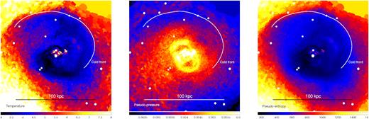
Projected thermodynamic maps. Left: projected temperature map in the unit of keV. Middle: pseudo-pressure map. Right: pseudo-entropy map. The position of the cold front which delineates the spiral pattern shown in Fig. 1 right is shown in white. The white circles are the positions of point sources which are visually identified and subtracted.
3 RESULTS
3.1 Global morphological features
In the unsharp-masked image (Fig. 1 left) and the relative deviation image (Fig. 1 right), we see plenty of structures. Since many of the features have already been mentioned and explored in the literature (e.g. Churazov et al. 2000, 2003; Fabian et al. 2006; Sanders & Fabian 2007; Sanders et al. 2016), here we point out the structures which are related to our subsequent detailed analyses.
In the relative deviation image, we see a clear spiral-like pattern which has been discussed in the literature (e.g. Churazov et al. 2003; Fabian et al. 2006; Sanders & Fabian 2007; Sanders et al. 2016). Delineating the outer edge of the spiral, we see a brightness edge which starts about 50 kpc west of the core and extends anticlockwise to about 70 kpc north-east of the core in the unsharp-masked image. This spiral-like structure and the edge are also apparent in the projected temperature and pseudo-entropy maps (Fig. 2). The fact that the gas beneath the edge is cooler and has lower entropy than above the edge, as well as the fact that no clear pressure structure along the edge is seen, indicate that the edge is a cold front, originating from the sloshing motion of cool gas in the core (Ascasibar & Markevitch 2006; Markevitch & Vikhlinin 2007).
In addition to known structure, we identify two new structures; (1) The west half of the front seems relatively smooth, while the east half of the front exhibits a more complex, double-layered structure, indicating the existence of developing instability which may be due to the sloshing motion of the ICM. We point out the similarity between this cold front and the low-viscosity numerical simulation result by Roediger et al. (2013b, see the middle panel of fig. 3 of Roediger et al. 2013b). They attributed this phenomenon to the difference of mean shear at different azimuths of the front; (2) In the unsharp-masked image, underneath the west half of the front, we see feather-like structures, namely alternating bright and faint regions which have not been reported previously in the literature. Recently Werner et al. (2016a) found similar structures just below the northwestern cold front in the Virgo cluster. Wang & Markevitch (2018) also reported similar narrow ‘channels’ in the surface brightness image of Abell 2142.
3.2 Double-layered structure of the eastern cold front
Fig. 3 shows the close-up view of the eastern part of the cold front, where we see a peculiar double-layered structure. The overlaid partial annuli are adjusted so that their curvature matches the curvatures of the two fronts.
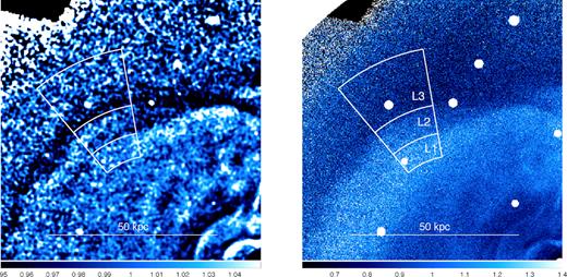
Same as Fig. 1, zoomed in on the double-layered structure. White partial annuli denote the regions along which the surface brightness profile and X-ray spectra are extracted.
The extracted surface brightness profile is shown in Fig. 4 top left. In order to estimate the positions of the breaks, we fitted the surface brightness profile using a projected double-broken power-law model following the procedure presented by Ichinohe et al. (2017). The centre of spherical symmetry is set to the concentre of the sectors shown in Fig. 3 left. The model describes the profile well with χ2/DOF = 40.7/37 and strongly prefers the double-broken power-law model to the single-broken power-law model by Δχ2/ΔDOF = 104.5/3. The positions of the two breaks are r12 = 82.5 ± 1.0 arcsec and r23 = 107.0 ± 0.5 arcsec, respectively, for the inner and outer breaks. These error ranges are overlaid in Fig. 4 as the grey vertical bands.
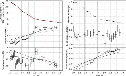
Top left: surface brightness profile extracted across the double-layered structure. The red curve is the best-fitting projected double-broken power-law model. Top right: pseudo-density profile. Middle left: projected temperature profile. Middle right: projected Fe abundance profile. Bottom left: pseudo-pressure profile. Bottom right: pseudo-entropy profile. The solid/dashed curves are reference profiles calculated using the azimuthally averaged profile over 60°–180°/the entire azimuths. The grey vertical bands denote the positions of the breaks in the surface brightness profile. The radial distance from the centre at which all the plots start is ∼2.5 arcmin.
We also extracted thermodynamic profiles along the sectors shown in Fig. 3 left. The spectral fitting was performed in the same manner as was done for the thermodynamic maps (Fig. 2). The resulting (pseudo-) thermodynamic profiles are shown in Fig. 4.
We also plotted reference profiles in the temperature, the pressure and the entropy panels, using the azimuthally averaged temperature, pseudo-pressure and pseudo-entropy profiles. We split the entire field of view into an annular grid with radial and azimuthal intervals of 10 arcsec and 10°, respectively, which are concentred on the cluster centre. From each grid element, we extracted spectra and analysed them in the same way mentioned in the paragraphs above, resulting in thirty six thermodynamic values per radial annulus. We averaged them to obtain the radial thermodynamic profiles. Since the projected pressure map shows a significant asymmetry as shown in Fig. 2, we calculated the averaged thermodynamic profiles in two ways; (1) averaged over all the azimuths and (2) averaged over the azimuthal range of 60°–180°. The reference profiles based on the average over all azimuths are plotted using the dashed curves and the ones using the azimuthal range of 60°–180° are plotted using the solid curves in Fig. 4.
Although almost continuous, we see some indications for the change in slope and the existence of a mild jump around the first break in both the temperature and entropy profiles. These profiles show a rapid increase towards the second break, and flatten out beyond the second break. These profiles are systematically lower than the reference profiles and seem to overtake the reference profiles around the second break. While the pressure profile is continuous at the first break, it shows 10–15 per cent jump at just outside the second break and monotonically decreases beyond the second break; the overall pressure profile is non-monotonic and a dip is seen between the two breaks. The Fe abundance is almost constant over the entire radial range.
3.3 Feather-like structures
Fig. 5 shows the same images as Fig. 1, zoomed-in to the vicinity of the feather-like structures, together with the SDSS r-band optical image (Eisenstein et al. 2011; Ahn et al. 2014). The alternating bright and faint regions are clearly seen in the unsharp-masked image (left-hand panel). Among the structures which are apparent in the unsharp-masked image, the central faint region (brightness dip; denoted by the white polygon in the leftmost panel) exhibits the most prominent contrast against the surrounding ICM, which even can be seen in the lower contrast relative deviation image (the polygon with the annotation ‘F2’ in the middle panel).
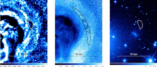
The close-up view of the unsharp-masked image (left), the relative deviation image (middle), and the SDSS r-band optical image of the corresponding sky region. The regions employed in a detailed study of the brightness dip are overlaid on the relative deviation image. These regions are numbered from F1 to F3 from north to south.
To investigate the ICM properties in the brightness dip in detail, we chose the regions based on the relative deviation image, because the unsharp-masked image is essentially an edge-enhanced image and thus is not suitable for considering the absolute brightness of the structures. We number these regions from F1 to F3 from north to south (see Fig. 5 middle). The areas of the regions F1 and F3 are double compared to that of the region F2 for each radius, lessening the uncertainty due to the difference of the radial dependence of the region shape between the regions.
For each region, we extracted spectra and fitted the data with an absorbed single temperature thermal plasma model; phabs(apec). We modelled each region independently allowing all the parameters to vary except for the redshift. The resulting parameters are shown in Table 1. Although the normalization shows a clear deficit with respect to the surroundings in the brightness dip region (region F2), we do not see significant deviations of the other quantities. Note that we also tried to model these regions using two temperature model, but the parameters were not well constrained.
Best-fitting parameters of the single temperature model in the ‘feathers’ region. (a) Calculated using ε/S where ε is apec normalization and S is the region area in arcsec2.
| Region | Temperature (keV) | Fe abundance (solar) | Area-normalized apec norma (10−6) | nH (1022 cm−2) |
|---|---|---|---|---|
| F1 | 3.81 ± 0.03 | 0.85 ± 0.02 | 3.49 ± 0.03 | 0.154 ± 0.002 |
| F2 | 3.89 ± 0.05 | 0.88 ± 0.04 | 3.15 ± 0.04 | 0.151 ± 0.004 |
| F3 | 3.96 ± 0.03 | 0.86 ± 0.02 | 3.53 ± 0.03 | 0.149 ± 0.002 |
4 DISCUSSION
4.1 Double-layered structure
As shown in Section 3.2, the projected double-broken power-law model represents the surface brightness profile around the eastern part of the cold front (Fig. 3) better than the single-broken power-law model does. Although the best-fitting parameters other than the break radii are uncertain because the assumption of the spherical symmetry in the projection is probably inaccurate, at least qualitatively the underlying density profile must then also host a double-layered structure similar to the surface brightness profile or the images.
4.1.1 Kelvin–Helmholtz instability
Generally, at a shock front, when the density shows a jump, the temperature, pressure, and entropy also show a jump, because a shock front propagating through the ICM heats and compresses the gas behind it. In contrast, since cold fronts are merely the interface between a cold gas parcel and hot ambient medium, when the density exhibits a drop, the temperature and entropy exhibit a jump, resulting in an almost continuous pressure profile across the front.
As shown in Fig. 4, both at the first and the second breaks, the density decreases but the temperature and entropy increase, which indicates that neither feature is a shock front. Especially, despite the jumps of temperature and entropy, the pressure is almost continuous at the first break, suggesting that this represents a (mild) cold front. At the second break, on the other hand, the change of slopes (rapid increase to flat) of the temperature and entropy profiles is associated also with a jump in the pressure, suggesting this structure is not a cold front in the classical sense.
Such a situation can be realized when Kelvin–Helmholtz instabilities (KHIs) are developing on top of the cold front: the first break was originally a cold front due to the sloshing motion of the gas induced by a previous merger event, which currently manifests itself with the spiral-shaped morphology. Due to the shearing motion of the gas, KHIs have been set off and are currently developing, and the second break represents the envelope of current maximum heights of the KH eddies. Since the KHIs mix the gas inside the front into the ambient gas, the contrast of the initial cold front is being weakened, and the thermodynamic properties inside and outside the first break are not strongly discontinuous. Since KHI eddies are not as coherent as the cold front, we would not detect a clear jump of temperature or entropy at the second break but would observe continuous changes of thermodynamic profiles, which is what our results actually show. A simplified cartoon of this situation is schematically drawn in Fig. 6. It should be noted that the sloshing cold front is itself a wave phenomenon that propagates outwards in the stratified atmosphere, therefore the fluid structure at the interface is in fact different than the shear interface realized in simple, two-dimensional parallel-flow set-ups. 3D numerical simulations of gas sloshing demonstrate that KHI with properties very similar to our observations develop even in the conditions of this more complex flow pattern (Roediger et al. 2013a).
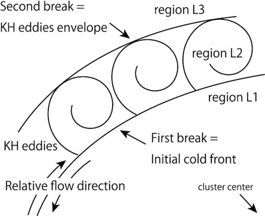
Schematic illustration of the double-layered structure due to the developing KHIs on top of the sloshing cold front. The region numbers correspond to the ones in Fig. 3 right. Note that the outward motion of the cold front is not represented in this simplified cartoon.
In order to test this scenario, we examined the multitemperature properties of the corresponding regions. We combined the sectors below the inner break, between the two breaks, and above the outer break (regions L1, L2, and L3, respectively). These regions are shown in Fig. 3. We extracted spectra using these regions and fitted them using single-temperature (1T; phabs(apec)) and two-temperature (2T; phabs(apec + apec)) models. Note that three-temperature modelling does not improve the fit. In addition to the independent fitting, we also model the spectra in all the regions simultaneously, with the two temperatures, Fe abundance and nH tied together.
Table 2 shows the fitting results. While every region prefers the 2T modelling (ΔCstat/ΔDOF = 91.4/2, 89.8/2, and 82.6/2 for regions L1, L2, and L3, respectively), letting the temperature, Fe abundance, and nH in all the regions vary independently does not significantly improve the fitting (ΔCstat/ΔDOF = 10.79/8), which suggests all the regions share the same two temperatures. Moreover, the ratio of the normalization of the cooler component to that of the hotter component (ε2/ε1) increases towards the cluster centre (regions L3 to L1). This supports the interpretation of the double-layered structure being a developing KHI, where the hotter component represents the ambient medium, while the cooler component represents the gas which is originally inside the cold front, being mixed into the ambient medium via the currently developing KHI.
Summary of the two-temperature fitting results for the double-layered structure. (a) apec normalization; ε = 10−14∫nenHdV/4π[DA(1 + |$z$|)2] where DA is the angular diameter distance to the source (cm), ne and nH are the electron and hydrogen ion densities (cm−3).
| Fitting condition | kT1 (keV) | ε1 (10−3)a | kT2 (keV) | ε2 (10−3)a |
|---|---|---|---|---|
| 1T, region L1 | 4.53 ± 0.04 | 1.36 ± 0.01 | – | – |
| 1T, region L2 | 5.21 ± 0.04 | 1.50 ± 0.01 | – | – |
| 1T, region L3 | 6.75 ± 0.05 | 2.57 ± 0.01 | – | – |
| 2T, region L1 | |$6.36_{-0.42}^{+0.52}$| | 0.92 ± 0.10 | |$2.62_{-0.20}^{+0.17}$| | 0.47 ± 0.10 |
| 2T, region L2 | |$9.03_{-1.18}^{+0.98}$| | |$0.80_{-0.32}^{+0.17}$| | |$3.40_{-0.32}^{+0.39}$| | |$0.72_{-0.17}^{+0.19}$| |
| 2T, region L3 | |$8.34_{-0.28}^{+0.97}$| | |$2.21_{-0.34}^{+0.09}$| | |$2.94_{-0.32}^{+0.96}$| | |$0.37_{-0.09}^{+0.29}$| |
| 2T, region L1 (comb) | |$8.37_{-0.24}^{+0.27}$| | 0.59 ± 0.05 | |$3.23_{-0.11}^{+0.09}$| | 0.78 ± 0.05 |
| 2T, region L2 (comb) | – | 0.89 ± 0.05 | – | 0.63 ± 0.05 |
| 2T, region L3 (comb) | – | |$2.15_{-0.07}^{+0.06}$| | – | |$0.44_{-0.06}^{+0.07}$| |
| Fe abundance (Solar) | nH (1022 cm2) | Cstat/DOF | ||
| 1T, region L1 | |$0.78_{-0.02}^{+0.03}$| | 0.160 ± 0.002 | 624.8/467 | |
| 1T, region L2 | 0.79 ± 0.03 | 0.160 ± 0.002 | 730.8/467 | |
| 1T, region L3 | 0.77 ± 0.02 | 0.158 ± 0.002 | 911.6/467 | |
| 2T, region L1 | 0.72 ± 0.03 | 0.163 ± 0.003 | 533.4/465 | |
| 2T, region L2 | 0.81 ± 0.03 | 0.159 ± 0.003 | 641.0/465 | |
| 2T, region L3 | 0.81 ± 0.03 | 0.157 ± 0.002 | 829.0/465 | |
| 2T, region L1 (comb) | 0.79 ± 0.02 | 0.159 ± 0.001 | 2014.1/1403 | |
| 2T, region L2 (comb) | – | – | – | |
| 2T, region L3 (comb) | – | – | – |
Using numerical simulations, Roediger et al. (2013b) indeed showed that KHIs can be induced along the edge of the sloshing spiral under certain conditions (particularly in low-viscosity cases), and that in such cases, the surface brightness profile hosts characteristic multiple edges, similarly to our case. It is also suggested by Roediger et al. (2013a,b) that the distance between the edges is about a fourth to a half of the scale length of the KH rolls. In our case, the distance between the two breaks is 25 ± 1 arcsec, corresponding to the actual distance of 8.8 ± 0.4 kpc, while the azimuthal extension of the double-layered structure is 30–40 kpc, which is consistent with the prediction from the simulation. Therefore, we suggest that this double-layered structure originates from the sloshing cold front accompanied by developing KHIs.
Our detection joins a growing number of indications for the existence of KHI suggested recently. For example, a similar multiple-edge structure in the merger cold front of the NGC 1404 galaxy has been reported by Su et al. (2017), and the existence of both the multiple-edge structure and the possible pressure deficit (see also the next section) has been presented also for the merger cold front in Abell 3667 (Ichinohe et al. 2017). Werner et al. (2016b) found multiple sloshing-induced cold fronts in the core of the Ophiuchus cluster and proposed that they could be due to KHIs. Walker et al. (2017) has suggested the existence of another giant KHI roll at ∼150 kpc south-east from the core in association with the outer cold front of the Perseus cluster. Recently Wang & Markevitch (2018) found well-developed KH eddies in the southern cold front of Abell 2142.
4.1.2 Pressure deficit and non-thermal pressure support
Based on the KHI scenario, here we investigate the ICM microphysical properties. As is pointed out in Section 3.2, the pressure between the two breaks seems to be insufficient to balance the surrounding gas. Assuming that the gas is uniform over the LOS depth of L, the pseudo-density |$\tilde{n}$| is translated to the electron density value of |$n_\mathrm{ e} = 38\tilde{n}(L/63\,\mathrm{kpc})^{-1/2}\mathrm{cm}^{-3}$|, where 63 kpc corresponds to the approximate distance of the structure from the cluster centre (∼3 arcmin). Similarly, the physical value of the pressure deficit Δp corresponding to the deficit of pseudo-pressure |$\Delta \tilde{p}\sim 0.1\times 10^{-3}$| is Δpe ∼ 3.8 × 10⁻³ keV cm−3(L/63 kpc)−1/2.
In the case of the two-temperature modelling (see Table 2), assuming that the cooler component of the gas inside region L1 is uniform over the LOS depth of L1, the normalization of the apec ε1 is translated to the physical density value of n1 ∼ 1.4 × 10⁻²(L1/63 kpc)−1/2cm−3. Similarly, that of the hotter component ε2 is translated to n2 ∼ 7.0 × 10⁻³(L2/334 kpc)−1/2cm−3, where 334 kpc corresponds to the core radius rc = 15.85 arcmin of the best-fitting β-model for the northeastern direction obtained by Urban et al. (2014). Accordingly, the pressure of each component is estimated at p1 ∼ 4.4 × 10⁻²(L1/63 kpc)−1/2keV cm−3 and p2 ∼ 5.9 × 10⁻²(L2/334 kpc)−1/2keV cm−3.
Although there are geometrical uncertainties, in both cases, the electron pressures seem to disagree with each other by a value of order 10−2 keV cm−3, with the gas between the two breaks or the cooler component having a lower pressure.
There are some candidates which can support the pressure deficit. The first one is magnetic pressure (e.g. Keshet et al. 2010). In this case, assuming that the pressure deficit is fully supported by the magnetic pressure, B2/8π = Δp yields the magnetic field strength of B ∼ 30 |$\mu$|G, where p = (ne + ni)kT is the pressure, assuming equal temperature between electrons and ions, and ne = 1.2ni. Reiss & Keshet (2014) found a thermal pressure jump of ∼10 per cent in a sample of 17 cold fronts in relaxed clusters not including Perseus. If the Perseus cold front is in fact located at the second break, our estimated pressure deficit of a similar magnitude is consistent with their scenario. However, our interpretation is that the real location of the cold front corresponds to the first break in the surface brightness profile instead.
As gas sloshing induces gas motion, turbulent pressure can be another candidate. In this case, assuming the turbulence to be isotropic, |$\rho V_\mathrm{1d}^2 =\Delta p$| leads to the one-component turbulent strength of V1d ∼ 400 km s−1, where the mass density ρ = μmpne with mp being the proton mass and μ = 0.6 being the mean particle weight.
The forming eddies themselves can also contribute to the pressure deficit because the central part of a vortex has lower pressure than its outer parts. This mechanism can have a significant impact especially in the early stage of the development of KHIs when the eddies remain coherent. It is difficult to distinguish these two mechanisms (turbulence and eddy) from the current observation. Direct measurement of the emission line width with future calorimeter observations of this region using e.g. XRISM (Tashiro et al. 2018) and Athena (Barcons et al. 2015) would be thus interesting regarding the origin of this feature and also more generally the pressure component at work in the cores of galaxy clusters.
KH eddies collapse into smaller-scale eddies and ultimately dissipate into heat, and the gas will be turbulent during the dissipation. Therefore, it is interesting to estimate whether or not the turbulent heating can balance the radiative cooling at this radius, assuming that the current size of the structure and the current turbulent strength represent the driving scales of turbulence. According to Zhuravleva et al. (2014), the turbulent heating rate Qturb can be estimated using |$Q_\mathrm{turb}=C_\mathrm{Q}\rho V_\mathrm{1d}^3/l$|, where CQ ∼ 5 is a fiducial constant related to the Kolmogorov constant and may differ by a factor ∼2, V1d is the one-component velocity of the turbulence, and l is the corresponding spatial scale. Using l = 30–40 kpc and V1d ∼ 400 km s−1, the heat input rate can be estimated at Qturb ∼ 3 × 10⁻²⁶ erg cm−3 s−1.
On the other hand, the cooling rate of the gas Qcool = Λneni is estimated at 1–2 × 10⁻²⁷erg cm−3 s−1, where Λ is the normalized cooling function calculated in Sutherland & Dopita (1993), with the temperature of several keV and approximating the ICM as having a Solar metal abundance. Considering the uncertainties (e.g. geometry and the value of CQ), we can only suggest that this cooling rate is comparable to ≲Qturb, meaning that the turbulent heating is able to balance the radiative cooling.
The magnetic pressure support and the turbulent pressure support can coexist, and it is difficult to disentangle the two factors. However, it is worth pointing out that our estimated value of Qturb ∼ 3 × 10⁻²⁶ erg cm−3 s−1 agrees within an order of magnitude with the previous estimation of Qturb ∼ 10−26 erg cm−3 s−1 (Zhuravleva et al. 2014), although these two calculations are performed on the same target but in a completely different way: the previous estimation by Zhuravleva et al. (2014) has been done using the surface brightness fluctuations in a statistical manner, while we estimate it thermodynamically from a single distinct substructure. This may indicate the importance of turbulent heating regarding the cooling problem of cluster cores.
The result indicates that the turbulence triggered by sloshing-induced KHIs may have non-negligible contributions to the ICM turbulence, which has not been considered extensively based on the observational perspective. It is possible that the gravitational energy injected by minor mergers supports the heat input into the ICM because gas sloshing is easily triggered by minor mergers that are constantly happening during the growth of galaxy clusters. We though note that there is no way to regulate heat input from minor mergers to exactly balance cooling, and thus it cannot be the only mechanism.
Recently, Hitomi Collaboration (2016) and Hitomi Collaboration (2018) have measured the LOS velocity dispersion of the gas in the core of the Perseus cluster at ∼100–200 km s−1. Our estimated turbulent strength is higher than this value. However, there are many uncertainties regarding the comparison; first, the region that we used for the turbulent estimation is not covered by the Hitomi observations. Also, the turbulent scales that the two observations probed may be different from each other. Secondly, our estimated value is based on the assumption of isotropy, which is probably not correct because KHIs occur along a shear flow, which has a certain direction (in the plane of the sky and not in the LOS in our case). Thirdly, how each turbulent component that originates from each turbulent driver (e.g. AGN or sloshing) contributes to the total turbulence may be different between the two observations.
4.1.3 Convergent flows
Although the azimuthal average of the temperature and the entropy profiles (see Fig. 4) increase monotonically towards the larger radii, the profiles along the double edge considered here do not seem to follow them. Instead, the temperature and the entropy profiles seem flat beyond the second break. At the same time, they may also indicate a signature of flattening between the first and the second break (1.4–1.6 arcmin).
These profiles indicate the existence of convergent gas flows at the second break, where the hot and high-entropy gas is moving inwards from the outside and the cold and low-entropy gas is moving outwards from the inside. Such convergent gas flows around sloshing cold fronts have been observationally suggested (Werner et al. 2016a) and also actually indicated in the numerical simulations (e.g. Ascasibar & Markevitch 2006; Roediger et al. 2011). The reason of the flattening of the thermodynamic profiles inside the second break being not as clear as those outside the second break may be the complex gas flow due to the developing KH eddies. The pressure enhancement above the second break may also be related to the compression due to convergent flows.
4.1.4 Weak shock
Inside the first break around 1.2 arcmin, a pressure break is seen. It is also seen independently in temperature, density, and entropy profiles. The higher temperature side has the higher density, which indicates that this is a weak shock front. It is possible that this feature is related to the sloshing cold front in some way, but it is more likely that it is related to the inner ripple-like structures.
4.2 Brightness dip
As shown in the optical image in Fig. 5, we do not see any corresponding optical structures around the brightness dip region, suggesting the brightness dip is purely an ICM substructure, i.e. not a structure generated by stars or galaxies, but simply due to the distribution of the diffuse gas. The temperatures of the three regions agree with each other (see Table 1), which indicates that the brightness dip region is unlikely to be associated with a temperature structure such as shock-heated or adiabatically compressed gas.
The brightness dip is apparently dark, and the fitting results suggest that the normalization at the dip is lower than the surroundings. Therefore, we suggest that the brightness dip is most probably a region where the gas, whose properties are similar to the surroundings, is simply depleted in terms of the LOS volume or the density.
4.2.1 Magnetic field strength
Based on the gas depletion scenario, here we investigate the microphysical properties of the ICM. As shown in Fig. 1, the feather-like structures exist just beneath the western cold front. We point out the similarity of these structures to the recent numerical simulations of the gas sloshing of magnetized plasma (e.g. ZuHone, Markevitch & Lee 2011; ZuHone et al. 2015; Werner et al. 2016a). The simulations suggest that when a tangential flow due to the sloshing motion exists and the plasma is magnetized, the magnetic fields therein are stretched and amplified along the flow direction even if the magnetic fields were initially tangled. The stretched magnetic fields push out the gas around them with the amplified magnetic pressure, resulting in a fluctuation of the surface brightness which represents the alignment of the magnetic fields inside the projected volume of the ICM.
Assuming that the ICM is uniform in each region and has an LOS depth of L, the deficit of the area-normalized apec normalization of ∼0.4 × 10⁻⁶ shown in Table 1 is translated to the deficit of the electron density of Δne ∼0.002 cm−3(L/42 kpc)−1/2, where 42 kpc is the distance of the brightness dip from the cluster centre (∼2 arcmin). Given the temperature uniformity, the physical density deficit directly indicates the deficit of the electron pressure Δpe ∼ 0.01 keV cm−3(L/42 kpc)−1/2(kT/3.9 keV), where kT is the gas temperature, which should be supported by some other pressure component(s) different from thermal pressure.
Considering the apparent similarity between the Perseus cluster (e.g. Fig. 1) and the numerical simulation result by Werner et al. (2016a) as well as other results of magnetized gas sloshing simulations in the literature (e.g. ZuHone et al. 2011, 2013), the most natural physical mechanism operating to support the gas pressure is magnetic pressure. The Δp = B2/8π relation immediately yields the magnetic field strength B ∼ 30 |$\mu$|G(L/42 kpc)−1/4(kT/3.9 keV)1/2.
The estimated magnetic field strength of ∼30 |$\mu$|G seems rather high, considering that the ambient magnetic field in the ICM has been estimated at around several |$\mu$|G (Carilli & Taylor 2002; Bonafede et al. 2010, 2013). However, there have been simulations which suggest that the ambient magnetic field can be amplified by some factors from several |$\mu$|G, especially in the clusters which show dynamical activity such as gas sloshing (e.g. ZuHone et al. 2011, 2013, 2015). Actually this value is measured only for the dip and not representative of average magnetic field strength in bulk of ICM, and given that the Perseus cluster indeed shows many signs of dynamical activity we think this estimation is not implausible. Note that even for the ambient values, there have been observations which indicate ambient ICM magnetic field strengths of ≲40 |$\mu$|G (e.g. Taylor & Perley 1993; Allen et al. 2001; Carilli & Taylor 2002). Also, there have been observations which indicate magnetic field strengths of 20–70 |$\mu$|G (e.g. Taylor et al. 2007; Fabian et al. 2008; Werner et al. 2013) in H α filaments.
4.2.2 Other candidates for the pressure support
The above scenario where the brightness dip is attributed to the magnetic fields amplified due to the gas motion is consistent with previous studies and simulations. However, other sources of pressure, such as non-thermal pressure support by relativistic particles or turbulent pressure support by gas motions, may also play a role. Importantly, we cannot reject some of these other scenarios, at least with the current observations.
Current radio data (70–600 MHz, compiled in Gendron-Marsolais et al. 2017) do not show any clear distinct feature at this location. However, one viable alternative scenario is that the brightness dip is a ghost bubble which represents a past activity of the central active galaxy, similarly to the other brightness cavities shown in Fig. 1. Since such ghost cavities simply push out the gas, the resulting thermodynamic structure should be similar to the case of magnetic field amplification. However, given its relatively small size compared to the other bubbles, we do not think this is the case, because if the gas depletion were due to the ghost cavity, it would have had time to expand to the size similar to the other cavities, during its buoyant uplift.
Turbulence is another candidate, but it seems unlikely that turbulence is localized to within such a small and clearly confined region. We can in principle test this scenario by measuring the width of the emission lines using high-resolution spectroscopy.
5 CONCLUSIONS
In this paper, we studied substructures associated with the sloshing cold front in the core of the Perseus cluster using ∼1 Msec archival Chandra ACIS-S data. The main results of our work are summarized below.
We find that the west half of the cold front seems relatively smooth, while the east half of the front exhibits a more complex, double-layered structure. We point out the similarity between this cold front and recent low-viscosity numerical simulations of KHIs in the context of gas sloshing.
We find that the surface brightness profile across the double-layered front has two brightness edges, which is predicted by numerical simulations of KHIs along the sloshing cold front. We measure the thickness of the layer to be 8.8 ± 0.4 kpc and the azimuthal extension of the layer to be 30–40 kpc, whose ratio is also consistent with the prediction from the numerical simulation.
We find that the thermodynamic structure across the double-layered front is consistent with it being a developing KHI layer along the sloshing cold front.
We find a pressure deficit in the thermodynamic profile at the corresponding radii of the KHI layer candidate. Assuming the LOS geometry, we estimated that the pressure deficit is of the order of 10−2 keV cm−3.
If the pressure is fully supported by turbulent pressure, the turbulent strength is estimated at V1d ∼ 400 km s−1, which is within an order of magnitude of previous estimations using other complementary methods. Assuming that the current size of the structure and the current turbulent strength represent the driving scale of the turbulence, we estimated the turbulent heating rate at Qturb ∼ 3 × 10⁻²⁶ erg cm−3 s−1, which can balance the radiative cooling at this radius. It indicates the importance of turbulent heating regarding the cluster cooling problem, and at the same time that the turbulence triggered by sloshing-induced KHIs may have non-negligible contribution to the ICM turbulence.
We find feather-like structures underneath the west half of the front, which are similar to the structures that emerge in the recent numerical simulations of the gas sloshing of magnetized plasma.
The thermodynamic properties of the brightness dip, the clearest of the feather-like structures, are consistent with it being the projected gas depletion layer induced by the amplified magnetic field.
Based on this scenario, we estimated the amplified magnetic field strength at B ∼30 |$\mu$|G.
ACKNOWLEDGEMENTS
YI is supported by Rikkyo University Special Fund for Research (SFR). AS gratefully acknowledges support by the Women In Science Excel (WISE) programme of the Netherlands Organisation for Scientific Research (NWO), and is thankful to the Kavli Institute for the Physics and Mathematics of the Universe for their continued hospitality. NW is supported by the Lendület LP2016-11 grant awarded by the Hungarian Academy of Sciences. ACF acknowledges support from ERC Advanced Grant 340442.
Footnotes
CIAO Homepage, Data Preparation; http://cxc.harvard.edu/ciao/threads/data.html
