


ABSTRACT
In 2015–2016, the X-ray nova A0620−00 in quiescence was observed in the passive state, according to the terminology of Cantrell et al., and in less than 230 d it transited into the active state. The system mean luminosity increased by 0.20 mag in the optical and by 0.25 and 0.30 mag in J and K infrared bands, respectively, while the orbital light curves changed drastically, and the flickering amplitude more than doubled. The mean light-curve analysis performed in the context of two models argued that the interaction region where the gas stream reaches the disc is responsible for these effects. The growth of this region’s luminosity in the active state implies the increase of the mass transfer rate via the L1 point, likely due to non-stationary processes in the donor star atmosphere. The non-stellar spectrum Fλ in the observed range |$\lambda \lambda 6400\hbox{--}22\, 000$| Å obeys a power law of λα where α = −(2.13 ± 0.1) in the passive state and α = −(1.85 ± 0.1) in the active, while the absolute mean square flickering amplitude behaves like ΔFfl(λ) ∼ λ−2.36 in both states of activity.
1 INTRODUCTION
X-ray novae with black holes (BHs) provide us with a majority of information on the masses of stellar-mass BHs (see e.g. Casares & Jonker 2014). These are soft X-ray transients that display violent outbursts of X-ray and optical radiation which last for several months. In intervals between eruptions, the binary system is observed to be X-ray quiescent and has the X-ray luminosity LX < 1033 erg s−1. The principal mechanism responsible for the optical and infrared (IR) brightness variability is the ellipticity of the optical star (Lyutyi, Sunyaev & Cherepashchuk 1973, 1975). As the luminosity of the optical star in low-mass X-ray binaries (LMXRBs) is relatively low, the zone where the gas stream interacts with the accretion disc (interaction region) provides a significant part of emission, and so do the relativistic jets, whose synchrotron radiation causes the observed IR polarisation (Russell et al. 2006, 2016). That is why the regular orbital flux variation due to the ellipticity effect is modulated by different kinds of additional variability induced by a change in gas parameters. This pattern may be further altered by the optical star physical variability and complicated by starspots on its surface (see e.g. Khruzina & Cherepashchuk 1995; Zurita et al. 2016).
The decade-long observations of X-ray binaries reveal the following types of additional brightness variations superimposed over the orbital optical and IR light curves (Cantrell et al. 2008; Casares & Jonker 2014):
The so-called superhump variability which affects the orbital light curve and arises due to the precession of the accretion disc semimajor axis which happens during an outburst and even in quiescence.
Fast aperiodic and quasi-periodic variability with an amplitude from a few to tens per cent on time-scale from a few seconds to tens of minutes, which is usually called flickering. Flickering is commonly thought to be related to magnetohydrodynamic processes in the accretion disc, in the stream–disc interaction region and, perhaps, to some non-stationary processes in relativistic jets.
The nature of flickering is not yet well established (see e.g. Bruch 2000, 2015; Baptista 2015). This type of activity is observed in dwarf novae, polars, symbiotic stars, and X-ray binaries. In recent year, the flickering properties of accreting objects have been studied intensively. For example, Zamanov et al. (2015) have traced flickering activity of the recurrent nova RS Oph in quiescence and point out that flickering amplitude increases as the mean system flux rises; the effect is also observed for X-ray binaries (Gandhi 2009).
According to Cantrell et al. (2008), three distinct optical states can be distinguished for some LMXRBs being in X-ray quiescence – passive, loop, and active, – that represent various levels of activity. As the object transitions from the passive to active state, the mean system brightness goes up and the irregular variability amplitude increases. The photometric observations of the A0620−00 = V616 Mon system in 2003–2016 by Shugarov, Katysheva & Gladilina (2015) and Shugarov et al. (2016) trace such an optical light-curve evolution consisting of periods characterized by relatively regular brightness variations (the passive state) and periods when the ellipsoidal orbital light curve is disturbed by irregular flares, corresponding to the active state.
As a rule, the passive-state binary displays the lowest flickering intensity. It is the ellipticity effect which is the dominating source of variability during the passive state of quiescence (Cantrell et al. 2008, 2010). The orbital inclination i derived from the analysis of passive-state light curves is considered the most reliable.
The A0620−00 system has been observed for more than 40 yr and by now is studied thoroughly (see the review of Casares & Jonker 2014 and references therein). Nevertheless, in recent years essentially new data have been obtained evidencing the fast change in orbit period (Gonzalez Hernandez et al. 2004, 2017). Moreover, the quiescent system has been found to display variable linear IR polarization (Russell et al. 2016). It makes necessary to continue intensive multicolour photometric and spectral observations of A0620−00.
In this paper, we examine the wavelength dependence of the mean total light flux, orbital light-curve shape, and flickering amplitude as well as the spectrum of non-stellar component in the range from 6400 Å to |$2.2 \mu \mathrm{m}$| for the system being in the passive and active states of quiescence. In Section 2, we present the photometric data for A0620−00 in the optical white light and in the J and K near-IR bands. Section 3 describes the model for the system and methods of light-curve interpretation. Section 4 presents the restored spectra of non-stellar component and in Section 5, the flickering parameters are determined. In Section 6, we summarize our main findings and make final conclusions.
2 OBSERVATIONS
Observations of A0620−00 = V616 Mon were performed during two winter seasons of 2015–2016 and 2016–2017 in the optical and near-IR wavebands. Each night it was possible to monitor the system for approximately half an orbital period. The observation log is given in Table 1.
Log of optical and IR-observations of A0620−00.
| Date | JD | N | φi − φf | mmin | mmax | Telescope | Series |
|---|---|---|---|---|---|---|---|
| dd.mm.yyyy | 2450000 + | mag | mag | m | number | ||
| 04.11.2015 | 7331.435–.653 | 399 | 0.389–1.063 | 3.010 | 2.535 | 1.25 | ΔC331 |
| 05.11.2015 | 7332.449–.653 | 376 | 0.529–0.158 | 2.938 | 2.621 | 1.25 | ΔC332 |
| 16.12.2015 | 7373.447–.528 | 7 | 0.451–0.701 | 2.902 | 2.680 | 1.25 | ΔC373 |
| 22.12.2015 | 7378.521–.544 | 3 | 0.158–0.230 | 2.826 | 2.785 | 1.25 | ΔC378 |
| 22.12.2015 | 7379.295–.531 | 19 | 0.557–1.287 | 2.978 | 2.664 | 1.25 | ΔC379 |
| 03.01.2016 | 7391.306–.591 | 139 | 0.739–1.621 | 2.024 | 2.662 | 0.6 | ΔC391 |
| 31.01.2016 | 7419.182–.346 | 161 | 0.039–0.547 | 15.545 | 15.408 | 2.5 | J419 |
| 31.01.2016 | 7419.188–.344 | 154 | 0.058–0.540 | 14.608 | 14.440 | 2.5 | K419 |
| 02.02.2016 | 7421.216–.408 | 182 | 0.335–0.932 | 15.527 | 15.366 | 2.5 | J421 |
| 02.02.2016 | 7421.221–.397 | 170 | 0.351–0.897 | 14.484 | 14.364 | 2.5 | K421 |
| 03.02.2016 | 7422.233–.448 | 201 | 0.486–1.151 | 15.537 | 15.334 | 2.5 | J422 |
| 03.02.2016 | 7422.238–.453 | 183 | 0.501–1.164 | 14.529 | 14.331 | 2.5 | K422 |
| 29.03.2016 | 7477.258–.366 | 55 | 0.835–1.168 | 2.909 | 2.557 | 0.6 | ΔC477 |
| 31.03.2016 | 7479.267–.334 | 39 | 0.054–0.261 | 2.974 | 2.705 | 0.6 | ΔC479 |
| 19.11.2016 | 7711.503–.662 | 236 | 0.020–0.509 | 2.717 | 2.204 | 1.25 | ΔC711 |
| 19.11.2016 | 7712.475–.659 | 341 | 0.028–0.597 | 2.770 | 2.229 | 1.25 | ΔC712 |
| 20.11.2016 | 7713.400–.661 | 454 | 0.892–1.700 | 2.930 | 2.273 | 1.25 | ΔC713 |
| 21.11.2016 | 7714.430–.514 | 140 | 0.080–0.340 | 2.753 | 2.237 | 1.25 | ΔC714 |
| 22.11.2016 | 7715.436–.658 | 387 | 0.194–0.883 | 2.834 | 2.347 | 1.25 | ΔC715 |
| 30.11.2016 | 7723.441–.546 | 183 | 0.976–1.301 | 2.925 | 2.221 | 1.25 | ΔC723 |
| 05.12.2016 | 7728.455–.549 | 136 | 0.500–0.791 | 2.815 | 2.266 | 1.25 | ΔC728 |
| 23.01.2017 | 7777.264–.493 | 159 | 0.603–1.313 | 2.856 | 2.402 | 0.6 | ΔC777 |
| 26.01.2017 | 7780.344–.527 | 127 | 0.139–0.704 | 2.807 | 2.379 | 0.6 | ΔC780 |
| 27.01.2017 | 7781.294–.421 | 70 | 0.079–0.475 | 2.870 | 2.502 | 0.6 | ΔC781 |
| 28.01.2017 | 7782.290–.326 | 36 | 0.163–0.277 | 2.727 | 2.520 | 0.6 | ΔC782 |
| 16.02.2017 | 7801.189–.414 | 213 | 0.672–1.370 | 15.492 | 14.982 | 2.5 | J801 |
| 16.02.2017 | 7801.194–.410 | 202 | 0.688–1.355 | 14.240 | 14.007 | 2.5 | K801 |
| 19.02.2017 | 7804.220–.408 | 190 | 0.056–0.636 | 15.351 | 15.599 | 2.5 | J804 |
| 19.02.2017 | 7804.225–.413 | 190 | 0.071–0.652 | 14.198 | 14.018 | 2.5 | K804 |
| 06.03.2017 | 7819.148–.337 | 210 | 0.272–0.856 | 14.312 | 14.054 | 2.5 | K819 |
| 06.03.2017 | 7819.163–.352 | 203 | 0.317–0.901 | 15.388 | 16.061 | 2.5 | J819 |
Notes. Date is a UT date for the beginning of observation; JD denotes the observational interval during current night; N – number of observations; φi, φf – orbital phases corresponding to the beginning and end of monitoring; mmin, mmax – minimal and maximal brightness during the observing period (the observed differential magnitude ΔC of A0620−00 with respect to its primary comparison star in white light filter, and J and K magnitudes in the near-IR). In the last column, we designate the data series as filter and monitoring night number (as JD−2457000) which is used to distinguish data in the light curves in Fig. 2. Photometric data will be published later and are available upon request.
2.1 Near-IR observations
IR observations in the J (|$\lambda _{\textrm{eff}}\sim 1.25 \mu \mathrm{m}$|) and K (|$\lambda _{\textrm{eff}}\sim 2.2 \mu \mathrm{m}$|) bands of the Mauna Kea Observatories (MKO) photometric system were performed at the newly installed 2.5-m telescope of Caucasian highland observatory of SAI MSU (Sternberg Astronomical Institute, Lomonosov Moscow State University), located in the Karachay-Cherkess Republic of Russia, at an elevation of 2112 m a.s.l. The site started operating in 2015 and was described in Sadovnichyi & Cherepashchuk (2015), while its astroclimatic parameters were analysed by Kornilov et al. (2014).
For IR observations, the ASTRONIRCAM camera spectrograph (Nadjip et al. 2017) with the Hawaii-2RG detector of 2048 × 2048 pixels and a set of wide-band filters was used. The camera operated in photometric mode in which only the central area of 1024 × 1024 pixel was used. The image plate scale was 0.27 arcsec pixel−1, the field of view was a 4.6 arcmin side square. Monitoring was performed with alternation of J and K filters every 9 or 10 exposures of 29.17 s during three nights in 2016 (January 31, and February 2 and 3) and three nights in 2017 (February 16 and 19, and March 3).
Resulting frame images were measured by the aperture photometry method with the primary comparison star 2MASS J06224334–0020262 which magnitudes were taken from the Two Micron All-Sky Survey (2MASS) catalogue and converted into the MKO system according to the calibration of Leggett et al. (2006) (JMKO = 13.247 mag and KMKO = 12.74 mag). The photometry precision was controlled using other comparison (control) stars close to the object both in magnitude and position (marked with numbers 2–6 in Fig. 1). No brightness correlation between comparison stars and the target was found; the root-mean-square (rms) error of the comparison star measurements varied between |$0{^{\rm m}_{.}}015$| and |$0{^{\rm m}_{.}}025$| depending on observing conditions on a particular night, so a value of |$0{^{\rm m}_{.}}02$| may be taken as a mean rms error estimate for the individual J, K-band measurements.
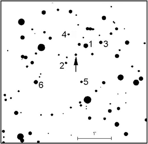
Finding chart for V616 Mon in the visible. 1 – primary comparison star (2MASS J06224334-0020262), and 2–6 – control stars.
The measured magnitudes were averaged within each filter series (over 3–9 points depending on observing conditions), thus yielding time sampling and photometric precision similar to those in the optical (see below). Such an averaging is believed to have no smoothing effect on measurements of flickering amplitudes since characteristic time of flickering for A0620−00 is of the order of 30–40 min (Shugarov et al. 2015, 2016). Thus, we obtained 125 averaged IR brightness estimates in 2016 and 434 estimates in 2017 which are used in the analysis presented in this paper.
2.2 Optical observations
Optical observations in white integral light [without filters, λeff ∼ 6400 Å, the bandpass half-response wavelengths are λλ4300–8300 Å, see e.g. Khruzina et al. (2015); Armstrong et al. (2013) for the discussion of the waveband] were taken at the 1.25-m telescope of the Southern station of SAI MSU (Crimea) equipped with a VersArray-1300B CCD (exposures of 45–60 s) and at the 0.6-m telescope of Slovak academy of sciences (Stará Lesná, Slovakia) equipped with a FLI ML 3041 CCD (exposures of 120 s). The object was observed on 2015 November 4 and 5, and December 16 and 22; 2016 January 3, March 29 and 31, November 19–22 and 30, and December 5; and 2017 January 23, and 26–28.
Images taken in white light were processed with the same comparison and control stars as used for IR observations (Section 2.1). The primary comparison star magnitudes are |$B=15{^{\rm m}_{.}}72$|, |$V=14{^{\rm m}_{.}}92$|, and |$R=14{^{\rm m}_{.}}2$| (see the catalogue of Cherepashchuk et al. 1996). The photometric intrinsic precision in white light (integral light, ‘Clear filter = C’) is about ∼0.01 mag which was assessed using rms deviation of differential magnitudes of the comparison stars, similarly to IR measurements. The number of independent magnitude estimates in white light was 1037 in the period from 2015 November to 2016 March and 2374 estimates for the time span from 2016 November to 2017 January.
2.3 Light curves
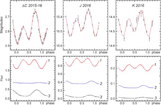
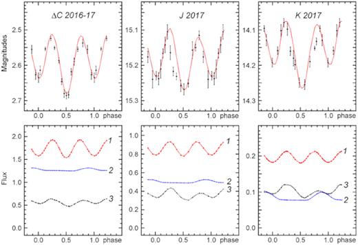
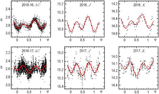
In Fig. 2, the photometric measurements in white light (ΔC is the differential magnitude with respect to the primary comparison star), as well as in the J and K bands, are given for two observational seasons: 2015–2016 and 2016–2017. The light curves for the first season exhibit regular orbital variability with relatively small scatter. The optical light curve for one orbital period represents a double wave with unequal maxima, with a φ = 1 minimum being deeper than that at φ = 0.5. This property is evident in the J and K light curves as well.
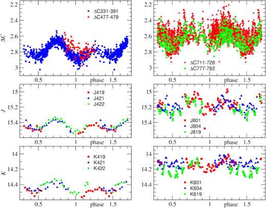
Photometric data on A0620−00 for the passive (2015–2016, left) and active (2016–2017, right) states folded with the orbital period. From top to bottom: ‘Clear filter’, and J and K bands. Different symbols refer to the data obtained during different nights (see Table 1).
The measurements for the 2016–2017 season presented in Fig. 2 are folded with the same orbital period. The double wave resulting from the optical star ellipticity is also well seen, but, unlike the first season, the primary and secondary maxima are roughly equal in height, while the φ = 1 minimum is shallower than that at φ = 0.5. Comparing the light curve with that of the 2015–2016 season, we see that the amplitude of irregular variability (flickering) has increased drastically. The mean brightness of the system has also increased in all the bands: by 0.2 mag in the optical, 0.25 mag in J, and 0.3 mag in K which is probably related to the increased contribution of the non-stationary accretion disc and synchrotron radiation of relativistic jets to the total light in 2017. The orbit-average J−K colour index is 0.79 in 2016 and 0.84 in 2017, i.e. the growth of flickering amplitude and mean brightness is accompanied by a little reddening of the system probably related to the synchrotron radiation impact. So, to judge by all the signs (see e.g. Cantrell et al. 2010; Casares & Jonker 2014) in 2016–2017 we witnessed the transition of A0620−00 from the passive state of quiescence to the active state, and it happened in less than 230 d. It is noteworthy that the relative flickering amplitude (in magnitudes) decreases only slightly from the optical to IR.
3 MEAN LIGHT-CURVE SIMULATIONS
Following in the footsteps of Cantrell et al. (2008), we managed to observe the A0620−00 system in two states of quiescence and to show that the transition between them had happened in less than 230 d. In order to shed light on the physical nature of the transition, we modelled the mean orbital light curves of this system in the context of two frameworks: a model with the dominating role of cool spots on the optical star (which is attractive given the recent discovery of extremely fast orbital period shortening detected for A0620−00, see Gonzalez Hernandez, Rebolo & Casares 2014), and a model with the stream–disc interaction region being the primary light modulation contributor apart from the ellipticity effect.
The modelling was performed with the fixed value of orbital inclination i = 51°, firmly constrained by Cantrell et al. (2010), the components mass ratio was q = Mx/Mv = 26 (Petrov, Antokhina & Cherepashchuk 2015, 2017; Antokhina, Petrov & Cherepashchuk 2017) which corresponds to the BH’s and optical star’s masses of |$M_\textrm{x}=6.5\, \mathrm{M}_{\odot}$| and |$M_\textrm{v}=0.26\, \textrm{M}_{\odot }$|, and a temperature of T = 4440 K was ascribed to the K3–K7V optical star (e.g. Froning, Robinson & Bitner 2007). The selected mass ratio is higher than q = 15 given by Marsh, Robinson & Wood (1994) for A0620−00, since the former was obtained within a more advanced model of rotational broadening of absorption lines in the optical star spectrum (Antokhina et al. 2017) and ties in better with the Doppler tomography results of Shahbaz et al. (2004). Though, it should be noticed that the light-curve interpretation weakly enough depends on q. Moreover, the new value q = 26 does not affect the BH mass but does slightly decrease the mass of the optical star.
The mean light curves of A0620−00 in all the observed wavebands were calculated by the standard method involving the splitting of the orbital curve into phase bins and calculating the mean luminosity and its error within each bin. Since the flickering contributes quite significantly into the observed variability and does not follow the normal distribution, such a procedure is not fully justified. Meanwhile, this simplified approach makes it possible to avoid subjectivity in outlining the lower envelopes of light curves (see e.g. Shahbaz et al. 2004; Zurita, Casares & Shahbaz 2003; Hynes et al. 2003) and, thus, to construct a formalised algorithm. The light-curve analysis involving the calculation of lower envelopes will be performed in a subsequent paper using additional observational data which are currently under accumulation.
3.1 Model with dark spots on the optical star: case (a)
Let us consider a model for the A0620−00 system with the dominating role of dark spots on the donor star surface, i.e. where the light contribution from the interaction region is neglected. This case was considered in details by Khruzina & Cherepashchuk (1995) with the use of a standard light-curve synthesizing algorithm which assumes a Planck spectrum for elementary areas on the accretion disc and donor star surface, the latter filling its Roche lobe. The gravity darkening is considered, the limb darkening is calculated in the linear approximation, while the X-ray heating of the donor star is neglected.
There are a number of reasons to apply such a model to the A0620−00 system. First, the chromospheric activity phenomenon was observed in several LMXRBs, including A0620−00 (Gonzalez Hernandez & Casares 2010; Zurita et al. 2003; Casares et al. 1997; Shahbaz et al. 2000; Torres et al. 2002). This is not surprising, since spots seem to be a common feature of late-type stars (e.g. Gershberg 2005) and were discussed in relation to LMXRBs by McClintock & Remillard (1990), Shahbaz, Naylor & Charles (1994), Khruzina & Cherepashchuk (1995), Gelino, Harrison & Orosz (2001), and Shahbaz, Watson & Dhillon (2014).
Secondly, extremely fast orbital period shortening discovered for A0620−00 (Gonzalez Hernandez et al. 2014, 2017; Ponti et al. 2017), to be explained in accordance with the standard evolutionary scenario (Iben, Tutukov & Yungelson 1995), requires huge magnetic fields on optical stars (several kilogauss) and such fields do exist in spots (Gershberg 2005).
Finally, the passive state light curves of A0620−00 demonstrate unequal maxima which are easily reproduced in synthetic curves if a dark spot is placed on one of the donor star’s hemispheres.
In our model with cool spots on the optical star and negligible influence of the interaction region (case a), the parameters to be found are those of two spots: the coordinates η, φ, the radii Rsp, and the temperature contrast Fsp = Tsp/Tstar < 1 determined for each spot relative to the local surface temperature; and those of the disc: the temperature Tin (at a radius of R1 = 0.0003a0 where a0 is the relative system orbit radius) and the αg parameter, which characterizes the surface distribution of the temperature: |$T(r)=T_\textrm{in}(R_1/r)^{\alpha _\textrm{g}}$|.
The outer radius of the accretion disc Rd was fixed at a value of Rd = 0.5ξ where ξ is the distance from the L1 point to the BH. This estimate is taken from the Doppler tomography analysis for A0620−00 (Marsh et al. 1994; Shahbaz et al. 2004).
In total, our case (a) model has 10 free parameters. To solve the inverse problem, the downhill method (Himmelblau 1972) is applied. While searching for the global minimum of residuals for each light curve, we tested several tens of initial approximations because of the known tendency of the residual functional to have many local minima when the number of parameters is high. The residual function was calculated as the sum of weighted squared deviations of the observed points from the model light curve; the χ2 criterion was used to select the best solution corresponding to the global minimum of the residual functional (for results, see Table 2, where the non-stellar component relative luminosity Fn/Fall is also given). The model light curves computed with these parameters, the components’ contributions to the total light (in arbitrary units) and a schematic representation of the system at different orbital phases φ are given in Figs 3 and 4. The flux from the compact object is negligible and not shown in the plots.
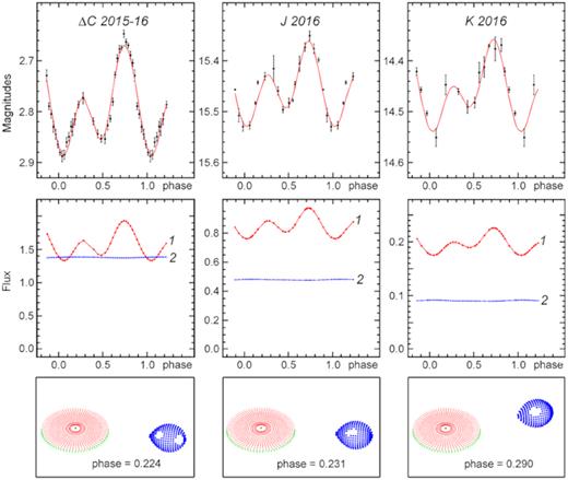
The spotted model of the passive-state A0620−00 system. Top panel shows the mean observed light curves (not corrected for interstellar extinction; points) and the simulated light curves. Middle panel represents the contribution of different components to the total light: donor star (1) and accretion disc (2). Bottom panel renders the model of the system at different orbital phases.
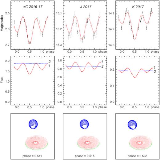
The spotted model of the active-state A0620−00 system. Panels and designations are the same as in Fig. 3.
Inverse problem solution for A0620−00 according to the model with spots (a).
| Parameter | |$C\, 2015-2016$| | |$J\, 2016$| | |$K\, 2016$| | |$C\, 2016-2017$| | |$J\, 2017$| | |$K\, 2017$| |
|---|---|---|---|---|---|---|
| Passive state | Active state | |||||
| Accretion disc | ||||||
| αg | 0.528(1) | 0.684(1) | 0.749(1) | 0.557(1) | 0.686(3) | 0.671(2) |
| Tin, K | 94 360 | 208 790 | 253 980 | 120 090 | 252 565 | 208 230 |
| ±320 | ±1 300 | ±1 300 | ±2 500 | ±2 500 | ±2 740 | |
| Cool spot 1 | ||||||
| Rsp/R2 | 0.37(1) | 0.19(9) | 0.35(4) | 0.35(4) | 0.49(6) | 0.35(4) |
| Fsp | 0.16(6) | 0.35(9) | 0.15(9) | 0.95(5) | 0.87(2) | 0.15(9) |
| η, ° | 143 ± 8 | 65 ± 34 | 70 ± 7 | 13 ± 5 | 13 ± 5 | 70 ± 7 |
| ϕ, ° | 147 ± 9 | 136 ± 13 | 132 ± 3 | 21 ± 15 | 94 ± 21 | 132 ± 3 |
| Cool spot 2 | ||||||
| Rsp/R2 | 0.32(3) | 0.25(9) | 0.20(9) | 0.32(3) | 0.25(9) | 0.20(9) |
| Fsp | 0.25(5) | 0.4(3) | 0.25(8) | 0.25(5) | 0.4(3) | 0.25(8) |
| η, ° | 51 ± 6 | 85 ± 34 | 94 ± 25 | 51 ± 6 | 85 ± 34 | 94 ± 25 |
| ϕ, ° | 131 ± 4 | 129 ± 10 | 126 ± 10 | 131 ± 4) | 129 ± 10 | 126 ± 10 |
| Fn/Fall | 0.464(5) | 0.358(4) | 0.314(4) | 0.534(7) | 0.496(5) | 0.501(5) |
| N | 32 | 18 | 13 | 16 | 17 | 15 |
| |$\chi ^2_{N,\, 0.10}$| | 53.7 | 34.8 | 27.7 | 32.0 | 33.4 | 30.6 |
| χ2 | 79.5 | 168 | 35.4 | 32.9 | 73.7 | 76.7 |
Notes. Solutions are obtained with the following parameters being fixed: |$T_2 = 4\, 440$| K, R2/a0 = 0.161, |$T_1 = 64\, 500$| K, and R1 = 0.0003a0. The latitude η is counted from the star ‘tip’ to the backside hemisphere and ranges from 0° to 180°; the longitude ϕ is counted from the orbital plane clockwise if looking from the relativistic object and changes from 0° to 360°. The relative input of the non-stellar component light is Fn/Fall and it does not depend on interstellar reddening; |$\chi ^2_{N,\, 0.10}$| is the chi-square value at the significance level of 10 per cent for a number of average points in the light curve N.
Table 2 also presents the formal errors which correspond to a 10 per cent increase of the minimal χ2 value. The minimal value itself is sufficiently higher than the critical value |$\chi ^2_{N,\,0.10}$| at 10 per cent evidencing that systematic errors are quite large due to the imperfection of the model and limited number of varying parameters. Nevertheless, the data in Table 2 and Figs 3 and 4 reveal that the spotted model is able to explain both passive- and active-states observed mean light curves of A0620−00, with each state being characterized by a different structure and location of spots on the donor star.
The restoration of the passive-state optical light curve yields two spots at similar longitude (ϕ ∼ 131° and 147°), but well separated in latitude (η ∼ 51° and 143°). Modelling IR passive light curves brings two spots with a small (∼20°) difference in latitude. Since the C observations were performed about 20 d earlier than the J and K ones, we may suggest that a real drift of the spot occurred during that period of time. The location of spots on one hemisphere of the optical star (at similar longitudes) appears to be able to account for unequal maxima in the passive light curves.
The active-state location of spots is similar for all three bands (white light, J and K filters); the spots are roughly merging into a large one located near the ‘tip’ of the tidally deformed donor star. Such a pattern explains well the deep minimum at the phase φ = 0.5 in the light curve.
For both states, the spots have radii of 20–50 per cent of the mean stellar radius, cover from 2 to 10 per cent of the stellar surface and have temperatures from 20 to 90 per cent of the star surface temperature. It should be stressed that the presence of spots may explain the shape of the light curves but not the rise of the average total luminosity from passive to active states (0.2–0.3 mag). For the change of total brightness to be explained, an independent growth of the accretion disc luminosity has to be assumed (see Figs 3 and 4).
Although the spotted model is capable to reproduce formally the observed mean light curves in both states of activity, the location of a large spot in the L1 point vicinity (which explains well the deep minimum near the phase φ = 0.5) contradicts with the increase of the disc luminosity observed in the active state, given our present understanding of the physics of the mass transfer in binary systems. Indeed, this large spot most likely consists of a set of pairs of smaller spots, and their strong magnetic fields (∼103 G) have an arc geometry and thus, on average, are oriented perpendicularly to the mass transfer direction. The gas outflow specific kinetic energy ρ|$v$|2/2 and the specific magnetic field energy H2/8π in the photosphere appear to be roughly equal if we assume a density of ρ = 10−6−10−7 g cm−3 for the photospheric gas, the starting outflow speed from the L1 point is |$v$| = 10 km s−1 (close to the local sound speed) and the magnetic field strength is H = (1 − 3) × 103 G. Therefore, the existence of a large spot on the star near L1 must considerably slow down the mass transfer from the star to the disc which in turn should decrease the non-stellar luminosity while what we observe is just the opposite. This contradiction implies that the spotted model is unable to explain adequately the total set of observational data on A0620−00 which forces us to consider an alternative model.
3.2 Model with a dominating role of interaction region: case (b)
Here, we make use of the model of an interacting binary system elaborated for the analysis of light curves of eclipsing cataclysmic systems (see Khruzina et al. 2001, 2003a,b; the detailed description can be found in Khruzina 2011). As in case (a), we implemented the classical light-curve synthesis, where the elementary areas on the star, disc, and stream–disc interaction region emit according to the Planck’s law at a local temperature; the parameters i = 51°, q = Mx/Mv = 26, Mx = 6.5 M|$\odot$|, Mv = 0.26 M|$\odot$|, and T = 4440 K are fixed, star spots are absent. The relativistic object is located in a focus of the elliptical accretion disc, whose eccentricity was fixed at a value of e = 0.1 as it is impossible to derive it from non-eclipsing light curves. The disc orientation is defined by the parameter αe that is the angle between the directions from the BH to the optical star and to the disc periastron and was also fixed at αe = 90°. The disc temperature distribution follows the same law as in the case (a).
The region where the gas stream interacts with the disc edge has a complex structure in our model. It consists of two components: a hotspot at the outer edge of the disc and a hotline (HL) outside the bright disc. The HL is a high-temperature part of the gas stream adjoining the hotspot on the leeward side. The stream matter is heated by the collision with the rotating disc and circumdisc halo and by a shock wave generated along that part of the stream where it joins the disc body. The HL phenomenon follows from the 3D gasdynamic simulations of the interacting binary systems (Bisikalo 2005; Lukin et al. 2017) which evidence that the stream interacts with the rotating disc in 3D model in a more complex way than the classical hotspot model predicts.
The idea that the gas stream may penetrate the accretion disc was first advanced by Chochol et al. (1984). Although the Doppler tomography results (Marsh & Horne 1988; Marsh et al. 1994) are not able to provide direct proof of the existence or absence of an HL, the restored Hβ emission-line images obtained by Shahbaz et al. (2004) render some extended structure of the stream–disc interaction region similar to an HL. Since a model including such a formation was also proved to be more successful in interpreting the light curves for cataclysmic binary systems than the model with a classical hotspot (see Khruzina et al. 2001, 2003a,b), we incorporate the HL in our present model of A0620−00.
In our model, the HL is approximated by a slanted ellipsoid with semi-axes av, bv, and cv and the hotspot – by a half-ellipse located on the outer edge of the disc, behind the HL. The ellipse centre coincides with the point of gas stream crossing the disc body.
There are seven free parameters: αg and Tin are the disc characteristics; av and bv – the semi-axes of an ellipsoid representing the HL (in the orbital plane); T25 andT75 – the temperatures in windward (towards the incoming flow) and leeward (behind the stream) regions of the HL; the ‘25’ and ‘75’ indices designate the orbital phases φ = 0.25 and 0.75, when these parts of the HL are best exposed to an observer; and the hotspot size Rsp which is the distance between the HL axis and the edge of the hotspot at the outer edge of the disc plus the heated part of the HL.
Table 3 and Figs 5 and 6 demonstrate the results of simulating the light curves of A0620−00 within the model with an HL. Fig. 7 shows the schematic images of the binary in the passive and active states. The χ2 values obtained in the HL model, like those of the spotted one, are well above the critical value |$\chi ^2_{N,\,0.10}$| at a significance level of 10 per cent. As in the spotted model, the limited number of free parameters and the necessity to describe light curves in all studied bands with the same fixed model parameters cause systematic deviation of simulated curves from the observed ones. Still we can admit that the model with an HL is able to reproduce the observed light curves not worse than the model with a spotty star.
The model with an HL. Passive state. Designations are the same as in Fig. 3. Here (3) is the HL luminosity.
The model with an HL. Active state. Designations are the same as in Fig. 3. Here (3) is the HL luminosity.
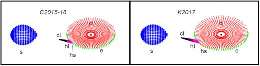
Plot showing a schematic representation of the A0620−00 system at an orbital phase of 0.75, as it appears in the model with an HL having the parameters from Table 3, being in the passive (left; the C band) and active (right; the K band) state. Different symbols depict the optical star (s), the internal (paraboloidal) part of the disc (d), the edge of the disc (e), the hotspot (hs), and the heated (hl), and cool (cl) parts of the HL.
Inverse problem solution for A0620−00 in frame of the model with an HL (b).
| Parameter | |$C\, 2015-2016$| | |$J\, 2016$| | |$K\, 2016$| | |$C\, 2016-2017$| | |$J\, 2017$| | |$K\, 2017$| |
|---|---|---|---|---|---|---|
| Passive state | Active state | |||||
| Accretion disc | ||||||
| αg | 0.670(1) | 0.705(1) | 0.749(1) | 0.483(1) | 0.553(4) | 0.600(8) |
| Tin, K | 192 555 | 219 275 | 231 570 | 71 140 | 94 445 | 92 505 |
| ±545 | ±580 | ±2 060 | ±435 | ±2 060 | ±4 300 | |
| Hotline | ||||||
| av/a0 | 0.024(1) | 0.024(1) | 0.02(1) | 0.027(1) | 0.025(2) | 0.027(3) |
| bv/a0 | 0.376(4) | 0.374(3) | 0.36(3) | 0.491(4) | 0.498(2) | 0.48(3) |
| T25, K | 7 535 | 7 710 | 7 200 | 8 645 | 19 650 | 47 205 |
| ±80 | ±235 | ±1 515 | ±195 | ±2 535 | ±5 465 | |
| T75, K | 10 595 | 11 105 | 11 120 | 7955 | 15 940 | 34 600 |
| ±150 | ±165 | ±1 090 | ±105 | ±720 | ±1 776 | |
| Hotspot | ||||||
| RHS/a0 | 0.046(1) | 0.26(1) | 0.39(1) | 0.2(1) | 0.13(9) | 0.2(2) |
| Fd/Fall | 0.280(2) | 0.287(4) | 0.268(6) | 0.360(2) | 0.290(1) | 0.216(5) |
| FHL/Fall | 0.099(6) | 0.040(3) | 0.024(2) | 0.155(3) | 0.211(5) | 0.268(7) |
| Fn/Fall | 0.379(6) | 0.326(5) | 0.292(6) | 0.515(4) | 0.501(5) | 0.484(8) |
| N | 32 | 18 | 13 | 16 | 17 | 15 |
| |$\chi ^2_{\textrm{N},\, 0.10}$| | 53.7 | 34.8 | 27.7 | 32.0 | 33.4 | 30.6 |
| χ2 | 60.0 | 37.1 | 68.7 | 104 | 121 | 179 |
Notes. Fd/Fall and FHL/Fall are the relative contributions of the disc with a hotspot and an HL, respectively, to the total light. On other parameters, see above, Table 2.
Let us look at the values obtained within the model with an HL (see Table 3). The HL semi-axis cv perpendicular to the orbital plane was fixed. Two other HL semi-axes, av and bv, which have a bigger impact on the total light of the system at the given inclination i = 51° than cv, appear to have the same values for all three photometric bands. In particular, av/a0 ∼ 0.024−0.027 in both states, while bv/a0 ∼ 0.37 in the passive state and increases up to ∼0.49 in the active one.
In the passive state, the HL colour temperature on the windward side is the same for all three bands within the errors (|$T_{25}\sim 7\, 500$| K); the same is seen for the leeward side (|$T_{75}\sim 11\, 000$| K). The T25 and T75 are of the same order of magnitude.
In the active state, the gas of the HL is hotter on the windward side than on the leeward side (T25 > T75) in all the bands which points out a strong shock wave propagating from the interaction region into the stream. Besides, the simulation yields a considerable increase in colour temperature of both parts of the HL with wavelength (from C to K) and also a rapid growth of the T25 − T75 difference: by ∼700 K in C, ∼3700 K in J, and ∼12500 K in K. It would thus appear that due to the steep stratification of temperature arising from the shock wave, and to the gas being less opaque in the IR than in the optical, we see hotter material in the IR than in the optical.
The temperature distribution along the disc radius is flatter for the active state (αg ∼ 0.48 in white light, 0.553 in J, and 0.60 in K) than for the passive one, αg ∼ 0.67 (C), 0.71 (J), and 0.75 in K. The temperature near the outer edge of the disc is ∼1900–2500 K in both states; and Tout is slightly higher at the disc periastron azimuth than at the apastron.
In the passive state, the HL luminosity in all the bands C, J, and K is lower than the luminosity of the accretion disc plus the hotspot (see Fig. 5 and Table 2). In the active state, the HL luminosity rises and in K the HL contribution to the non-stellar light becomes roughly the same as that of the disc with a hotspot (Fig. 6). It is tempting to consider the strengthening of the mass transfer rate from the donor star through the L1 point to cause the growth of the HL luminosity. Since the flickering amplitude increases significantly in the active state too, this rise may be related to the magnetohydrodynamic processes going on in the region where the gas stream interacts with the disc. The rise in ingress of matter into the disc causes the A0620−00 mean luminosity to increase by 0.2–0.3 mag (Fig. 2). It should be stressed though that the mechanism responsible for the energy release in the quiescent disc remains unclear (a nearly laminar accumulating disc, an advection-dominated disc, a disc with a strong wind, and relativistic jets, etc.).
All in all, the joint light-curve analysis for the passive and active states demonstrates the model with the dominating role of the interaction region to be adequate for the A0620−00 system. In the active state, the interaction region luminosity grows up which is naturally explained by increase of the gas outflow from the optical star through the L1 point. This rate depends on the Roche lobe overflow factor ΔR/RRoche where ΔR is the difference between the stellar photosphere radius and the mean Roche lobe radius.
One can see that |$\dot{M}$| strongly depends on ΔR (Masevich & Tutukov 1988). Hence, even small variations of ΔR related to, e.g. the supergranulation in the stellar atmosphere or the existence of active regions within it, may lead to considerable variation in mass transfer through the L1 point. This in turn will stimulate the transition of the system from the passive to the active state or backward. So, we may conclude that such active/passive state transitions in A0620−00 and, apparently, other similar systems in quiescence, may trace instability of the atmospheric parameters of a donor star.
4 NON-STELLAR COMPONENT SPECTRA
The non-stellar spectra of A0620−00 (the accretion disc plus the interaction plus jets) were derived in a number of works by means of subtraction of the donor star spectrum (or a comparison star of a similar type) from the observed dereddened system spectrum (Oke 1977; McClintock & Remillard 1986; McClintock, Horne & Remillard 1995; Shahbaz et al. 2004; Froning et al. 2011; Dinçer et al. 2018).
Cantrell et al. (2010) got a reliable estimate of the distance to A0620−00, d = 1.06 ± 0.12 kpc, for the mass ratio Q = Mv/Mx = 0.067. This allows calculating the flux density for the donor star outside the Earth atmosphere Eλ = πBλ(T)(Rv/d)2, where Bλ(T) is the Planck function, T and Rv are the temperature and radius of a K3−7KV star filling its Roche lobe. This flux varies with the phase of orbital motion due to the ellipticity effect with an amplitude depending on the orbital inclination i. The period-average flux of the donor star does not depend on i if we neglect the small effect of gravity darkening. So we restrict ourselves to the calculation of the period-average dereddened values of Eλ for the donor star and spectral flux density Fλ for the whole system A0620−00.
The observed C, J, and K magnitudes were corrected for the interstellar extinction using AV = 1.21 mag from Gelino et al. (2001) and the extinction law from Rieke & Lebofsky (1985). Calibrating optical measurements we made use of the fact that the effective wavelength ∼6400 Å of the C band is close to the central wavelength of the Johnson R band (∼7000 Å), so such a replacement was found appropriate.
Subtracting the donor-star flux Eλ from the dereddened total flux Fλ, we obtain the period-average stationary flux from the non-stellar component Hλ (accretion disc with the HL and hotspot plus the relativistic jets) as a function of wavelength λ.
On the other hand, it becomes possible to determine the stationary flux of the non-stellar component Hλ from the shape and amplitude of the mean orbital light curve obtained in frame of the given model of the binary system, since the orbital inclination is well defined: i = 51° ± 0|${^{\circ}_{.}}$|9 (Cantrell et al. 2010). The comparison of Hλ values derived from modelling light curves and from using the distance estimate is a good way to control the interpretation validity. In order to calculate the period-average donor-star flux Eλ, one can use the Eggleton formula for the relative Roche lobe radius RR (Eggleton 1983) and the third Kepler law to get the relative orbit radius. The average temperature of a K3–K7V optical star lies within the range of Tv = 4200–4700 K (Oke 1977; Habets & Heintze 1981; Gelino et al. 2001; Gonzalez Hernandez et al. 2004; Froning et al. 2007; Harrison et al. 2007).
The masses of the components are constrained by the reliably determined semi-amplitude of the radial velocity curve for the A0620−00 optical star, Kv = 433 ± 3 km s−1 (Marsh et al. 1994), and the estimate of the modified mass ratio Q = Mv/Mx, obtained from the rotational broadening of lines in the optical star spectrum. Marsh et al. (1994) applying the classical model of the rotational broadening (Wade & Horne 1988; Collins & Truax 1995) derived |$v$|sin i = 83 ± 5 km s−1 and Q ≈ 0.067. Applying a more sophisticated model of the optical star (Petrov et al. 2015, 2017; Antokhina et al. 2017) revealed a tendency for the classical model to overestimate the |$v$|sin i values and to yield higher Q. The relations given in above mentioned works allow correcting the mass ratios obtained within the classical model of broadening; for A0620−00 we got Q = 0.039. The respective masses of the BH and optical star turned out to be |$M_\textrm{x} = 6.5\, \textrm{M}_{\odot }$| and |$M_\textrm{v} = 0.26\, \textrm{M}_{\odot }$|. To trace the significance of an important choice of the broadening model, we used two values for the mass ratio in order to calculate the flux from the optical star: Q = 0.067 (|$M_\textrm{x} = 6.6\, \textrm{M}_{\odot }$| and |$M_\textrm{v} = 0.40\, \textrm{M}_{\odot }$|) and Q = 0.039 (|$M_\textrm{x} = 6.5\, \textrm{M}_{\odot }$| and |$M_\textrm{v} = 0.26\, \textrm{M}_{\odot }$|). Since the average radius of the donor star depends on Q, two distance estimates for A0620−00 are used as well: d = 1.06 kpc for Q = 0.067 (Cantrell et al. 2010) and d = 0.900 kpc for Q = 0.039.
Doppler tomography provides an additional argument for the use of lower mass ratio values Q < 0.067 for A0620−00 (Marsh et al. 1994; Shahbaz et al. 2004). Having constructed Doppler images of the Hα and Hβ emission lines, the authors noticed that the use of Q = 0.067 does not place the bright spot on either predicted gas stream path from the inner Lagrangian point L1, while smaller mass ratios bring the predicted path closer to the spot (Marsh et al. 1994).
In Table 4, the orbit-average fluxes Eλ of the donor star are given for λ = 6400, 12 500, and 22 000 Å. Calculations are performed for the temperature T = 4400 K and two values of modified mass ratio: Q = Mv/Mx = 0.067 and 0.039. The dispersion of the derived Eλ values gives an idea of the degree of uncertainty of these numbers.
Fluxes from A0620−00 averaged over the orbital period.
| λ | Fλ | Eλ | Hλ = Fλ − Eλ | Hλ/Fλ | Hλ/Eλ |
|---|---|---|---|---|---|
| Å | erg cm−2 s−1 Å−1 | erg cm−2 s−1 Å−1 | erg cm−2 s−1 Å−1 | ||
| d = 1060 pc, Q = 0.067 | |||||
| Passive state | |||||
| 6 400 | 8.007e−16 | 4.669−16 | 3.338−16 | 0.417 | 0.715 |
| 12 500 | 2.851e−16 | 2.132−16 | 7.190−17 | 0.252 | 0.384 |
| 22 000 | 7.447e−17 | 4.680−17 | 2.767−17 | 0.372 | 0.572 |
| Active state | |||||
| 6 400 | 9.662e−16 | 4.669−16 | 4.993−16 | 0.517 | 1.069 |
| 12 500 | 3.582e−16 | 2.132−16 | 1.450−16 | 0.405 | 0.680 |
| 22 000 | 9.748e−17 | 4.680−17 | 5.068−17 | 0.520 | 1.083 |
| d = 900 pc, Q = 0.039 | |||||
| Passive state | |||||
| 6 400 | 8.007e−16 | 4.941−16 | 3.066−16 | 0.383 | 0.621 |
| 12 500 | 2.851e−16 | 2.256−16 | 5.947−17 | 0.209 | 0.264 |
| 22 000 | 7.447e−17 | 4.952−17 | 2.495−17 | 0.335 | 0.504 |
| Active state | |||||
| 6 400 | 9.662e−16 | 4.941−16 | 4.721−16 | 0.489 | 0.955 |
| 12 500 | 3.582e−16 | 2.256−16 | 1.326−16 | 0.370 | 0.588 |
| 22 000 | 9.748e−17 | 4.952−17 | 4.796−17 | 0.492 | 0.968 |
Notes. Fλ – dereddened spectral flux density for the system.
Eλ – theoretical spectral flux density for a K3–K7V star at given d.
Hλ = Fλ − Eλ – dereddened spectral flux density for the non-stellar component (disc + hotline + hotspot + jets).
Hλ/Fλ – the fractional contribution of the non-stellar component to the total light.
Hλ/Eλ – the non-stellar component light to optical star light ratio.
For the C ≃ R, J, and K bands we used the calibration of Bessell, Castelli & Plez (1998): |$F_\textrm{R}^0=2.177\times 10^{-9}$|, |$F_\textrm{J}^0=3.147\times 10^{-10}$|, and |$F_\textrm{K}^0=3.961\times 10^{-11}$| in the units of erg cm−2 s−1 Å−1. The IR fluxes are estimated to be close to the data of Koornneef (1983).
In Table 4 are given the dereddened fluxes at λ = 6400, 12 500, and 22 000 Å for the passive and active states of A0620−00. The absolute average fluxes from the non-stellar component Hλ = Fλ − Eλ are listed as well as the fractional contribution to the total light Hλ/Fλ which could be directly compared to the values obtained via orbital light-curve modelling.
From modelling, we know the fractional contribution of every component into the total system luminosity at the wavelength of each photometric band in use (see Figs 3–6, all the fluxes are given in the same units). Having corrected the observed magnitudes for interstellar extinction and converted them into absolute units, we can obtain an absolute spectral energy distribution (SED) for the non-stellar component. On the other hand, we have estimated the non-stellar flux by subtracting the contribution of a tidally deformed K3–K7V star at given distances (1060 and 900 pc) from the total observed light corrected for interstellar extinction (see Table 4).
Fig. 8 shows the restored SEDs for the non-stellar component of A0620−00 in logarithmic scale for both states of activity. The four distributions were obtained by modelling the orbital light curves and by subtracting the stellar contribution calculated for two sets of Q and d values. The non-stellar spectra are well described by a power law: Hλ ∼ λ−2.13 ± 0.1 for the passive state and Hλ ∼ λ−1.85 ± 0.1 for the active state which match any of the Q, d choice (if an Hν ∼ νβ notation is concerned, then β = 0.13 ± 0.1 and −0.15 ± 0.1, respectively). It is remarkable that the Hλ functions derived by four independent methods correspond well to each other.
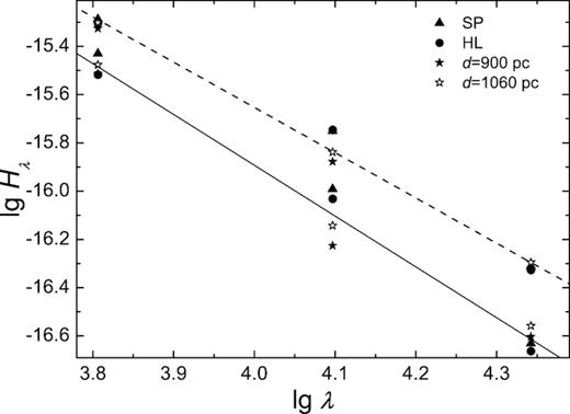
Restored spectra of the non-stellar component in the passive and active states in log–log scale. Triangles represent the spotted model (case a), circles – the HL model (case b), and filled and open stars – models with a |$T = 4\, 400$| K optical star and d = 900 and 1060 pc, respectively. Lines represent least-squares fits with slopes −2.13 for the passive (solid) and −1.85 for the active (dashed) state.
Our results are in accordance with the conclusions of Oke (1977; Fλ ∼ λ−2) and McClintock & Remillard (1986; Fλ ∼ λ−2.5 ± 1). The non-stellar spectrum Fλ ∼ λ−1.32 was restored by Dinçer et al. (2018) from the BVIJHK photometric data acquired in 2013 when, according to the authors’ opinion, A0620−00 was in the active state.
5 FLICKERING
Hynes et al. (2003) performed high time-resolution V-band photometry with exposures from 6 to 60 s and an accuracy of 0.8–1.7 per cent for a number of X-ray novae in quiescence. A0620−00 displayed some short flares with typical rise e-folding time-scales of less than 30–80 s and amplitudes of up to 10 per cent of the mean luminosity.
Shahbaz et al. (2004) carried out optical spectroscopy of A0620−00 and a spectrophotometric study of individual flares in this system with a duration from minutes to tens of minutes. The isolated spectrum of the flare may be fitted by a power law ∼λ−0.6 in the range λλ4452–7329 ÅÅ. The flare spectrum can also be interpreted as radiation from the optically thin gas with a temperature in the range 10 000–14 000 K that occupies 0.05–0.08 per cent of the disc surface. The flares may also arise from the bright spot at the outer edge of the disc.
Russell et al. (2016) performed polarimetric observations of A0620−00 and Swift 1357.2–0933 in the J, H, and Ks IR bands. For A0620−00, an excess of 1.25 ± 0.28 per cent linear polarization was measured and the magnetic field vector was found to be parallel to the axis of the resolved radio jet. The authors suggested that the polarization in the reddest bands is governed by the synchrotron emission from the jet present even in quiescence. The jet luminosity contributes up to ∼8–37 per cent of the Ks flux. Russell et al. also studied the variability of IR radiation in quiescence. The fractional rms variability amplitude constituted 1.84, 3.86, and 1.95 per cent in the J, H, and Ks bands, respectively, with a mean integration time of |${\sim }1300$| s for each band.
Recently Dinçer et al. (2018) fitted the flare spectrum for A0620−00 by the law λ−0.9.
In the present work, the photometric observations of A0620−00 in the visible and near-IR were performed for two activity states with the temporal resolution of a few minutes. The irregular variable component was extracted from the observed light curves fitted within a general multiparametric model (∼20 parameters). This enabled us to isolate flickering (together with observational errors) for different states of activity, orbital phases, and wavelengths in the range of |$\lambda \lambda 6\, 400\div 22\, 000$| ÅÅ.
In Fig. 9, the passive- and active-state observed light curves for A0620−00 are presented together with the simulated light curves. The respective residuals δ are shown in Fig. 10 in magnitudes for the visible and IR bands which include both the observational errors (∼0.01–0.02 mag) and a real physical variability (flickering) which is mostly higher than measuring errors.
Observed and simulated light curves of A0620−00 in the passive (top) and active state (bottom).
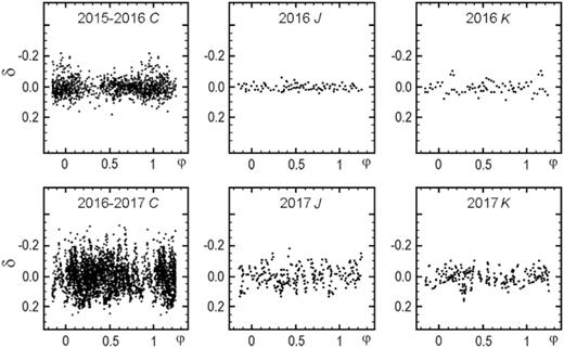
Residuals to the fits shown in Fig. 9 expressed in magnitudes for the passive (top) and active state (bottom).
It is evident from Fig. 10 that the flickering is mostly not phase-modulated with the possible exception of the optical range in the passive state where the flickering has a tendency to rise towards the phase φ = 0 (the X-ray source is behind the optical star).
The flickering amplitude is seen to depend on the activity state of the system. If expressed in magnitudes, the active flickering is twice as large as the passive one for all the bands. The active-state flickering is most prominent in the visible and its amplitude is comparable to that of the orbital variability of the system. The passive-state flickering amplitude varies with wavelength non-monotonically being minimal in J and rising again at longer wavelengths (K); this behaviour is similar to the one observed by Russell et al. (2016) (see above).
The flickering amplitudes for A0620−00.
| λ | Δmfl(λ) | ΔFfl × 1017 |
|---|---|---|
| Å | mag | erg cm−2 s−1Å−1 |
| 2016 | ||
| Passive state | ||
| 6 400 | 0.045 ± 0.001 | 3.308 ± 0.011 |
| 12 500 | 0.011 ± 0.003 | 0.296 ± 0.072 |
| 22 000 | 0.032 ± 0.005 | 0.217 ± 0.034 |
| 2017 | ||
| Active state | ||
| 6 400 | 0.093 ± 0.002 | 8.428 ± 0.181 |
| 12 500 | 0.060 ± 0.004 | 1.985 ± 0.141 |
| 22 000 | 0.047 ± 0.004 | 0.421 ± 0.033 |
Notes. Δmfl(λ) is the relative flickering amplitude averaged over the orbital period; and ΔFfl – the absolute rms flickering amplitude.
The active-state relative flickering amplitude Δmfl(λ) decreases monotonically from ∼ 0.093 to 0.047 mag with the wavelength changing from 6 400 to 22 000 Å. The passive-state flickering amplitude is significantly lower being 0.045 mag in C and 0.011 mag in J but increasing to 0.031 mag in K. The non-monotonic behaviour may be indicative of a two-component flickering structure which becomes visible in the passive state: the thermal component originating from flares in the disc and the disc–stream interaction region drops steeply from the visible (|$\lambda =6\, 400$| Å) to near-IR range (|$\lambda =12\, 500$| Å) and the non-thermal (synchrotron?) component dominates at longer wavelengths (i.e. at |$\lambda =22\, 000$| Å).
We fitted the wavelength dependence of the flickering amplitude ΔFfl (see Table 5) by a log-linear law |$\lg \Delta F_\textrm{fl}=K\lg \lambda +b$| independently for each state. K = −2.36 appears to fit both states while the standard error of K and chi-square criterion are σK = 0.13 and χ2 = 0.87 for the active state and σK = 0.44 and χ2 = 2.49 for the passive (with M = 3 degrees of freedom; see Fig. 11). This means that for both states of activity a power law gives a statistically adequate representation for flickering. This dependence is close to λ−2 that corresponds to the free–free emission of optically thin high-temperature plasma.
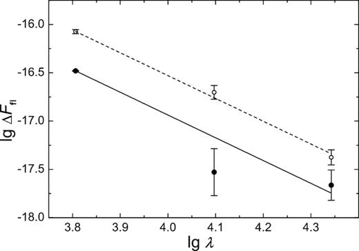
Plot showing the dependence of the absolute rms flickering amplitude on wavelength for A0620−00 in log–log scale. Filled symbols refer to the passive state, and open ones – to the active. The dependence is fitted by a linear law and is given by a solid line for the passive state and by a dashed one for the active.
As seen from Fig. 11, a unique law does not seem the best fit for the passive flickering amplitude. Considered separately, the exponents become λ−3.7 in the λλ6400–12 500 ÅÅ range and λ−0.6 in λλ12 500–22 000 ÅÅ which reflects the non-uniform decreasing of the flickering amplitude visible in Fig. 10. Meanwhile, a two-component structure of flickering to be confirmed, further observations involving more wavebands are required.
The absolute flickering amplitude ΔFfl(λ) grows for all wavelengths together with the mean system luminosity. This quantity also correlates with the non-stellar luminosity in the C, J, and K bands. This evidences that flickering in the A0620−00 system relates to non-stationary processes in the interaction region rather than to active regions on the donor star.
6 CONCLUSIONS
The high-precision (∼0.01–0.02 mag) photometric observations of A0620−00 (= V616 Mon) performed in 2015–2017 during quiescence in the visible (white light, λeff = 6400 Å) and in the J and K near-IR bands are presented and analysed. Below we summarize the main results of this study.
In 2015–2016, the system was observed to be in the passive state (according to the terminology of Cantrell et al. 2008, 2010) showing the regular orbital light curve in all the photometric bands with the flickering amplitude being significantly lower than the orbital modulation. In less than 230 d, the object transitioned to the active state: its mean magnitude grew by ∼0.2 mag in the C band, ∼0.25 mag in J, and ∼0.3 mag in K, the regular light-curve shape changed drastically while the flickering amplitude increased twice and became comparable to that of the regular orbital variability.
Given the orbital inclination fixed at i = 51° ± 0|${^{\circ}_{.}}$|9 (Cantrell et al. 2010) the light curves of A0620−00 were interpreted within two models of the binary system, namely, the one which assumes dark spots on the optical star and neglects the disc–stream interaction region, and the one which considers the contribution from the interaction region but not allows for spots on the optical companion.
The spotted model explains the observed inequality of maxima in the passive light curve (2015–2016) by a presence of two spots on the back side (relative to the orbital motion direction) of the donor star. The spots appear to cover ∼2–10 per cent of the stellar surface having radii of 0.2–0.5 of the mean stellar radius, while their temperatures turn out to be 0.2–0.9 of the mean surface temperature of the star.
During the active state (2017) both starspots are found to be located in the L1 point vicinity and their strong magnetic fields may thus depress the escape of the stellar matter via the gas stream. This contradicts to the observed increase in total and accretion disc luminosity in the active state. Therefore, the joint analysis of light curves in both states of activity allows us to reject the model with the dominating role of spots on the donor star for the A0620−00 system.
In the unspotted model, the appearance of the HL and hotspot in the disc varies with orbital phase and modulates the ellipsoidal light curve. The passive-state HL luminosity is lower than that of the accretion disc with a hotspot. In the active state, the HL contribution rises in all the studied bands. Since the active-state flickering is also much more intensive, such a growth may be related to the magnetohydrodynamic processes in the stream–disc interaction region. It is the rise in ingress of matter into the disc that is likely to cause the growth of non-stellar luminosity and the observed brightening of the system by 0.2–0.3 mag. It should be noticed though that the mechanism responsible for the energy release in the quiescent disc is still unclear.
Correcting the observed fluxes for interstellar extinction and taking into account the distance information from Cantrell et al. (2010) we subtracted the optical star contribution and reconstructed an orbit-average non-stellar spectrum in the λλ6400–22 000 ÅÅ wavelength range for both states of activity. These SEDs satisfactorily match the spectra restored from analysing the orbital light curves. The passive spectrum can be fitted by F(λ) ∼ λ−2.13 ± 0.1, while the active SED is described by F(λ) ∼ λ−1.85 ± 0.1 (F(ν) ∼ ν0.13 ± 0.1 and ∼ ν−0.15 ± 0.1, respectively). The non-stellar component contributes nearly ∼30 per cent to the passive-state total visible light and nearly ∼50 per cent to the active-state one.
The system being active the relative flickering amplitude Δmfl decreases monotonically from 0.093 to 0.047 mag with wavelength growing from 6400 to 22 000 Å. In the passive state, this quantity is significantly lower and depends on wavelength non-monotonically: Δmfl = 0.045 mag in the C band, 0.011 mag in J, and 0.031 mag in K, similarly to the finding of Russell et al. (2016).
The absolute rms flickering amplitude ΔFfl was fitted by a power law ∼λ−2.36 in the λλ6400–22 000 ÅÅ range for both states of activity (ΔFfl(ν) ∼ ν0.36 ± 0.1). The power-law index is close to that obtained for the restored spectrum of the regular non-stellar component in these states.
The correlation between the flickering amplitude and the mean system luminosity is manifested for all the studied bands and confirms the results of the previous studies of Cantrell et al. It evidences the increase in the contribution of the accretion disc and related structures into the total light. So, while A0620-00 remains in quiescence with a very low X-ray luminosity of ∼3 × 1030−2 × 1031 erg s−1 (Garcia et al. 2001; Dinçer et al. 2018) powerful non-stationary processes are going on in the system.
The absolute flickering amplitude ΔFfl(λ) in each photometric band is roughly proportional to the mean non-stellar luminosity.
Our general conclusion is that the transition of the quiescent A0620−00 system from the passive to the active state is likely related to the enhancement of mass transfer from the donor star through the L1 point, which depends strongly, as (ΔR/R)3, on the Roche lobe overflow factor for the donor star. Thus, we argue that the transition of A0620−00 between different activity states ‘traces’ the non-stationary processes in the donor star’s atmosphere.
ACKNOWLEDGEMENTS
This work was performed with the equipment purchased from the funds of the Program of Development of Moscow University. The effort of AMCh and NISh is supported by the Russian Science Foundation grant 17-12-01241 (problem formulation, IR observations and the analysis, and physical conclusions). NAK, TSKh, and SYSh thank the ‘Leading scientific schools’ program NSh-9670.2017.2 for the support (optical observations and computer modelling). SYSh thanks for partial support of his research by grants VEGA 2/0008/17 and APPV 15-0458 (optical observations). We also thank the anonymous referee for helpful suggestions which certainly improved the presentation of these results.
