


ABSTRACT
We use 85 pairs of high-resolution lambda cold dark matter (LCDM) cosmological simulations from the NIHAO project to investigate why in dwarf galaxies neutral hydrogen (H i) linewidths measured at 50 per cent of the peak flux W50/2 (from the hydrodynamical simulations) tend to underpredict the maximum circular velocity |${V_{\rm max}^{\rm DMO}}$| (from the corresponding dark matter only simulations). There are two main contributing processes. (1) Lower mass galaxies are less rotationally supported. This is confirmed observationally from the skewness of linewidths in bins of H i mass in both ALFALFA and HIPASS observations. (2) The H i distributions are less extended (relative to the dark matter halo) in dwarf galaxies. Coupled to the lower baryon-to-halo ratio results in rotation curves that are still rising at the last measured data point, in agreement with observations from SPARC. Combining these two effects, in both simulations and observations lower mass galaxies have, on average, lower W50/W20. Additionally, mass-loss driven by supernovae and projection effects (dwarf galaxies are in general not thin discs) further reduce the linewidths. The implied H i linewidth velocity function from NIHAO is in good agreement with observations in the nearby Universe of dwarf galaxies: |$10 \, {{ {\rm km\, s^{-1}} }} \lt W_{50}/2 \lt 80 \, {{ {\rm km\, s^{-1}} }}$|. The dark matter only slope of ≈−2.9 is reduced to ≈−1.0 in the hydro simulations. Future radio observations of unbiased samples with higher spatial resolution will enable stricter tests of the simulations, and thus of the LCDM model.
1 INTRODUCTION
The lambda cold dark matter (LCDM) model is very successful in reproducing the large-scale structure of the Universe (Springel et al. 2005) and the anisotropies in the cosmic microwave background (Planck Collaboration XVI 2014). In an LCDM universe there is a larger number of low-mass structures compared to more massive ones, or in other words a steeply declining halo mass function N(M) ∝ M−1 or halo velocity function N(V) ∝ V−3 (Klypin et al. 2015). This prediction is naively at odds with observational data around galaxies, i.e. the satellite abundance (Klypin et al. 1999; Moore et al. 1999). This ‘missing satellite’ problem has natural baryonic solution: galaxy formation becomes increasingly inefficient in low-mass dark matter haloes, due to the ionizing background, supernovae (SNe) explosions and gas removal due to ram pressure (Bullock, Kravtsov & Weinberg 2000; Benson et al. 2002; Kravtsov, Gnedin & Klypin 2004; Macciò et al. 2010). The latest cosmological hydrodynamical simulations of the Local Group are now consistent with the observed satellite stellar mass and velocity functions (e.g. Sawala et al. 2016; Buck et al. 2018).
The velocity function of galaxies using H i linewidths has been measured in the nearby universe (within ∼200 Mpc) from the HIPASS (Zwaan, Meyer & Staveley-Smith 2010) and ALFALFA surveys (Papastergis et al. 2011), and within the Local Volume (within 10 Mpc) by Klypin et al. (2015). These and other authors (Zavala et al. 2009; Trujillo-Gomez et al. 2011) have shown that LCDM provides very good estimates of the number of galaxies with circular velocities around and above |$80\, {{ {\rm km\, s^{-1}} }}$|. With a careful treatment of various systematics including survey selection effects, Obreschkow et al. (2013) showed agreement between LCDM down to circular velocities of |${\sim } 60\, {{ {\rm km\, s^{-1}} }}$|. However, LCDM appears to fail quite dramatically at lower circular velocities, overestimating by a factor of ≃3 the number of dwarf galaxies at velocity scale of |$50\, {{ {\rm km\, s^{-1}} }}$|, and by a factor of ≃5 at velocity scale of |$30\, {{ {\rm km\, s^{-1}} }}$| (Klypin et al. 2015). Galaxies at these velocity scales are essentially insensitive to the ionization background and, by not being satellites, they are not affected by gas depletion via ram pressure or by stellar stripping. This makes the mismatch between the observed linewidth function and the halo velocity function a more serious challenge to the LCDM paradigm. Furthermore, simple modifications to the LCDM paradigm, such as warm dark matter, are unable to resolve this issue as candidates with a warm enough particle to significantly reduce the number density of dark matter haloes result in a characteristic scale in the velocity function that is not observed (Klypin et al. 2015). The normalization of the velocity function is dependent on key cosmological parameters such as the amplitude of primordial perturbations (σ8) and the total matter density (Ωm) (Schneider & Trujillo-Gomez 2018). For example, the difference between a Planck (Planck Collaboration XVI 2014) and WMAP7 (Jarosik et al. 2011) cosmology is a factor of 1.43 in number density at fixed velocity (Klypin et al. 2015).
The solution to this discrepancy is that in dwarf galaxies H i linewidths measured at 50 per cent of the peak flux, W50, are a poor tracer of the maximum circular velocity of the host dark matter halo (Brook & Di Cintio 2015; Macciò et al. 2016; Brooks et al. 2017; Verbeke et al. 2017). This should not be a surprise, since it is generally known that lower mass and younger galaxies are less rotationally supported than higher mass, and older galaxies. This is seen in both observations (e.g. Kassin et al. 2012; Newman et al. 2013; Wisnioski et al. 2015), and hydrodynamical galaxy formation simulations (Ceverino et al. 2017; El-Badry et al. 2018). Furthermore, as discussed in Courteau (1997), unlike resolved H i rotation curves, H i linewidths do not necessarily sample outer discs effectively since the H i surface density drops rapidly beyond the optical radius.
In this paper we investigate the cause of the difference between W50/2 and |${V_{\rm max}^{\rm DMO}}$| further using galaxy formation simulations from the NIHAO project (Wang et al. 2015). Possible explanations we consider include: gas mass-loss from the halo – resulting in lower circular velocity in the hydro than dark matter only (DMO) simulation; H i in the simulations is not extended enough – so that the maximum rotation velocity does not reach the maximum circular velocity; non-circular motions – resulting in the rotation curve underestimating the circular velocity; projection effects – due to dwarf galaxies not being thin rotating discs.
The outline of the paper is as follows. Section 2 describes the cosmological hydrodynamical simulations and the various velocity definitions we use. In Section 3 we present the transformation from maximum circular velocity to H i linewidth. In Section 4 we present the implied H i velocity function from our simulations. In Section 5 we discuss what causes the linewidths to underestimate the maximum halo velocity, and present observational tests of these effects. A summary in given in Section 6.
2 SIMULATIONS
Here we give a brief overview of the NIHAO simulations. We refer the reader to Wang et al. (2015) for a more complete discussion. NIHAO is a sample of ∼ 90 hydrodynamical cosmological zoom-in simulations using the SPH code gasoline2 (Wadsley, Keller & Quinn 2017).
Haloes are selected at redshift |$z$| = 0 from parent dissipationless simulations of size 60, 20, and 15 Mpc h−1, presented in Dutton & Macciò (2014) which adopt a flat LCDM cosmology with parameters from the Planck Collaboration XVI (2014): Hubble parameter H0 = 67.1 |${\rm km\, s^{-1}}$| Mpc−1, matter density Ωm = 0.3175, dark energy density ΩΛ = 1 − Ωm = 0.6825, baryon density Ωb = 0.0490, power spectrum normalization σ8 = 0.8344, power spectrum slope n = 0.9624. Haloes are selected uniformly in log halo mass from ∼10 to ∼12 without reference to the halo merger history, concentration, or spin parameter. Star formation and feedback is implemented as described in Stinson et al. (2006, 2013). Mass and force softening are chosen to resolve the mass profile at |${\lesssim}1{{\ \rm per\ cent}}$| the virial radius, which results in ∼106 dark matter particles inside the virial radius of all haloes at |$z$| = 0. The motivation of this choice is to ensure that the simulations resolve the galaxy dynamics on the scale of the half-light radii, which are typically |${\sim } 1.5{{\ \rm per\ cent}}$| of the virial radius (Kravtsov 2013). Hydro particles have force softenings a factor of 2.34 smaller than the dark matter particles, and range from ≃75pc in the lowest mass haloes to ≃400pc in the most massive haloes.
Each hydro simulation has a corresponding DMO simulation of the same resolution. These simulations have been started using the identical initial conditions, replacing baryonic particles with dark matter particles. We remove the four most massive haloes (g1.12e12, g1.77e12, g1.92e12, g2.79e12), as these have formed too many stars, in particular near the galaxy centres, resulting in strongly peaked central circular velocity profiles (Wang et al. 2015). The final sample used in this work consists of 85 simulations.
Haloes in NIHAO zoom-in simulations were identified using the MPI + OpenMP hybrid halo finder AHF1 (Gill, Knebe & Gibson 2004; Knollmann & Knebe 2009). AHF locates local overdensities in an adaptively smoothed density field as prospective halo centres. The virial masses of the haloes are defined as the masses within a sphere whose average density is 200 times the cosmic critical matter density, |$\rho _{\rm crit} =3H_0^2/8\pi G$|. The virial mass, size, and circular velocity of the hydro simulations are denoted as M200, R200, and V200. The corresponding properties for the DMO simulations are denoted with a superscript, DMO. For the baryons we calculate masses enclosed within spheres of radius rgal = 0.2R200, which corresponds to ∼10 to ∼50 kpc. The stellar mass inside rgal is Mstar, the neutral hydrogen, inside rgal is computed following Rahmati et al. (2013) as described in Gutcke et al. (2017). In principle the neutral hydrogen should be separated further into atomic (H i), and molecular, (H2), gas. In practice this has only marginal impact on the derived H i linewidths. This is expected because in dwarf galaxies the ratio between molecular and atomic gas is very low, while in high-mass galaxies both atomic and molecular gas trace the same flat rotation velocity, albeit from gas at different radii. As a fiducial choice we consider atomic gas to be neutral gas with a density less than |$10\, {\rm cm^{-3}}$| (which is also the star formation threshold used in our simulations). We measure galaxy velocities using a number of definitions as discussed below.
The NIHAO simulations are the largest set of cosmological zoom-ins covering the halo mass range 1010–1012 M⊙. Their uniqueness is in the combination of high spatial resolution coupled to a statistical sample of haloes. In the context of LCDM they form the ‘right’ amount of stars both today and at earlier times (Wang et al. 2015). Their cold gas masses and sizes are consistent with observations (Stinson et al. 2015; Macciò et al. 2016), they follow the gas, stellar, and baryonic Tully–Fisher relations (Dutton et al. 2017), and they reproduce the diversity of dwarf galaxy rotation curve shapes (Santos-Santos et al. 2018). As such they provide a good template with which to connect galaxy observables (such as H i linewidths) to intrinsic properties of the host dark matter halo (such as maximum circular velocity).
2.1 Velocity definitions
We use a number of velocity definitions in this paper. We define them with the help of some examples as shown in Fig. 1. These galaxies were chosen to represent both rotationally supported galaxies (left-hand panels) and those with more pressure support (right-hand panels).
|${V_{\rm max}^{\rm DMO}}$| – maximum circular velocity of the DMO simulation. We start with the spherical circular velocity profile of the DMO simulation (solid black line), which is equivalent to the cumulative mass profile |$M(\lt r) = r\, V(r)^2/G$|. The maximum spherical circular velocity is shown as a black circle, and occurs at 15–25 per cent of the virial radius, R200 (upper axis scale).
Vmax – maximum circular velocity of hydro simulation. We next consider the circular velocity profile of the hydrodynamical simulation (blue lines). The solid line shows the spherical circular velocity, while the dashed line shows that derived from the potential in the disc plane, |$V^2_{\rm pot}=-R {\partial \Phi /\partial R}$|. We define |${V_{\rm max}}\equiv V_{\rm circ}(R_{\rm max}^{\rm DMO})$| as the spherical circular velocity of the hydro simulation at the radius where the maximum circular velocity of the DMO simulation occurs. We use this definition as it explicitly shows when there is mass-loss from the system (|${V_{\rm max}}\lt {V_{\rm max}^{\rm DMO}}$|), and where there is baryon dissipation (|${V_{\rm max}}\gt {V_{\rm max}^{\rm DMO}}$|). In these examples, there is mass-loss from the galaxies in the right-hand panels in Fig. 1, and no change for the galaxies in the left-hand panels.
Notice that the potential based circular velocity is lower than the spherical circular velocity at small radii, and higher at large radii. This is a well-known feature of the differences between a flattened and spherical mass distribution (Binney & Tremaine 1987)
VH i – circular velocity at H i radius. We define the H i radius, RH i, as enclosing 90 per cent of the H i mass (in the face-on projection). This approximates the edge of the observable H i rotation curve, and occurs close to the radius where the projected H i surface density profile reaches 1 M⊙ pc−2, but it has the advantage of being free from projection effects and is measurable in every galaxy (that contains H i). The potential based circular velocity at the H i radius is then, VH i ≡ Vcirc(RH i).
Vrot(R), σ(R) – rotation and dispersion profile. We calculate the rotation curve (red line), and dispersion profile (pink line) as follows. We rotate the galaxy to a face-on view, using the angular momentum of the cold (T < 15 000K) gas particles inside 10 per cent of the virial radius. We then divide the galaxy into a series of annuli of equal width. In each ring we calculate the mean velocity (Vrot) and velocity dispersion (σ) in the azimuthal (ϕ) direction. Note that this dispersion only takes into account the bulk motions of the gas. In the galaxies in the left-hand panels, the rotation velocity closely traces the potential based circular velocity, and the dispersion is low, |${\sim } 5\hbox{--}10\, {{ {\rm km\, s^{-1}} }}$|. In the galaxies in the right-hand panels, the rotation velocity systematically underpredicts the circular velocity, and the velocity dispersion is higher, |${\sim } 10\hbox{--}20\, {{ {\rm km\, s^{-1}} }}$|.
W50, W20 – H i linewidths. We next consider the H i linewidths, measured at 50 per cent and 20 per cent of the peak flux (see Fig. 2 for examples from our reference galaxies). In an update to the calculation in Macciò et al. (2016) here we include the thermal motions of the H i gas. At large linewidths the changes are minor, but for small linewidths the temperature adds a floor to the linewidth of |$~\sim 20\, {{ {\rm km\, s^{-1}} }}$|, corresponding to |$\sigma \sim 8.5\, {{ {\rm km\, s^{-1}} }}$|. For each gas particle we represent the line-of-sight velocity distribution with a Gaussian with mean corresponding to the line-of-sight velocity of the particle, a flux corresponding to the H i mass of the particle, and a dispersion computed from the temperature of the particle assuming |$\sigma =\sqrt{k_{\rm B}T/m_{\rm H}}=9.09 \,[{{ {\rm km\, s^{-1}} }}] \sqrt{T/10\,000 {\rm K}}$|. We sum up the Gaussians to give the flux versus velocity histogram.
As is commonly done in observations, we define the peak flux as the average of the peak flux on each velocity wing (i.e., positive and negative). See Fig. 2 for examples. The peak fluxes on each velocity wing are marked with dotted horizontal lines. The average of these is shown with solid horizontal lines. By definition W20 ≥ W50. Because W20 requires higher signal to noise, and thus can be measured from fewer galaxies, W50 is the more commonly used definition in large H i surveys, so will be our default definition.
We calculate the linewidths from 100 random projections (uniformly selected from the surface of a unit sphere), and measure the maximum, median, and minimum values. The maximum values typically correspond to the values derived from an edge-on view of the galaxy. They are shown as cyan (|$W_{20}^{\rm max}$|) and green (|$W_{50}^{\rm max}$|) horizontal lines in Fig. 1. The median W50/2 is shown with an orange horizontal line. The minimum linewidth (purple horizontal lines) can be used to approximate the gas velocity dispersion of the system, since for a Gaussian, σ = W50/2.35.
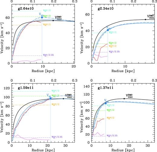
Example velocity profiles of four galaxies illustrating the different velocity definitions. The black line shows the spherical circular velocity of the DMO simulation. The black circle shows the maximum of this curve, |${V_{\rm max}^{\rm DMO}}$|, which typically occurs at |${\approx } 20{{\ \rm per\ cent}}$| of the virial radius, R200, (upper axis). The two galaxies in the upper panels have |${V_{\rm max}^{\rm DMO}}\sim 55\,{{ {\rm km\, s^{-1}} }}$|, while the galaxies in the lower panels have |${V_{\rm max}^{\rm DMO}}\sim 100\, {{ {\rm km\, s^{-1}} }}$|. The blue lines show the circular velocity of the hydrodynamical simulation using the spherically enclosed mass (solid lines) and the potential in the disc plane (dashed). The left-hand panels show galaxies where the rotation curve (red) traces the circular velocity from the potential (blue dashed), and the maximum linewidth W50/2 (green dashed line) equals the circular velocity at the H i radius, VH i (blue square). The right-hand panels show galaxies where the rotation curve underpredicts the circular velocity, and W50/2 underestimates VH i. The pink lines show the bulk velocity dispersion of the H i gas. A global measurement of the gas dispersion (including the thermal broadening) is given by the minimum H i linewidth / 2.35 (purple lines).
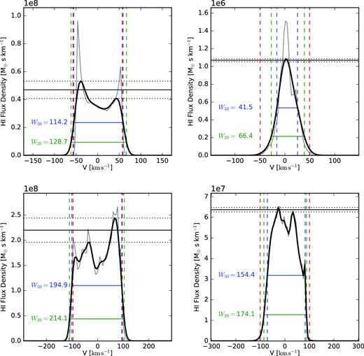
Example H i line profiles for edge-on projections of the four galaxies from Fig. 1 illustrating the different linewidth definitions. The black line shows the line profile including the thermal broadening, while the thin grey line shows the line profile from the kinematics only. The differences are only significant for the low-velocity haloes. The horizontal dashed lines show the peak fluxes from either velocity side, while the horizontal solid line shows the average peak flux. The 50 and 20 per cent peak fluxes are given with blue and green horizontal lines, respectively. The vertical blue and green dashed lines show the corresponding velocities at the 50 and 20 per cent peak fluxes. The red vertical line shows the maximum circular velocity of the dark matter halo, |${V_{\rm max}^{\rm DMO}}$|.
3 FROM MAXIMUM CIRCULAR VELOCITY TO H i LINEWIDTH
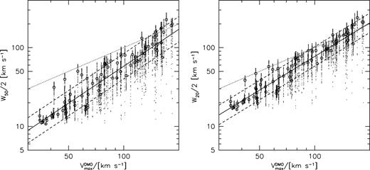
Relation between H i linewidths, W50 (left), and W20 (right) from the hydro simulations and maximum circular velocity from the corresponding DMO simulations. The points show 100 random projections per galaxy, with the open circle showing the median linewidth. The dotted line shows the one-to-one relation. The solid line shows a fit to all the data, with the 1σ scatter shown with dashed lines.
Fig. 4 shows the relations between various velocity definitions and |${V_{\rm max}^{\rm DMO}}$|. Linear fits (in log−log space) are given in Table 1. Notice that the normalization, slope, and scatter systematically change at each step. At anyone of these steps the changes are not large, but they accumulate to a relation between linewidth and halo velocity that is very different from a one-to-one correspondence. For galaxies in Milky Way mass haloes |${V_{\rm max}^{\rm DMO}}\simeq 180 {{ {\rm km\, s^{-1}} }}$| the average projected half-linewidth is |$W_{50}/2=141{{ {\rm km\, s^{-1}} }}$|, so that up to the expected project effects, the linewidth is a good tracer of the maximum halo velocity. However, for dwarf galaxies at |${V_{\rm max}^{\rm DMO}}\simeq 50{{ {\rm km\, s^{-1}} }}$| the average half-linewidth of |$W_{50}^{\rm med}/2 \simeq 20\,{{ {\rm km\, s^{-1}} }}$|, is a factor of 2.5 times lower than the halo velocity.
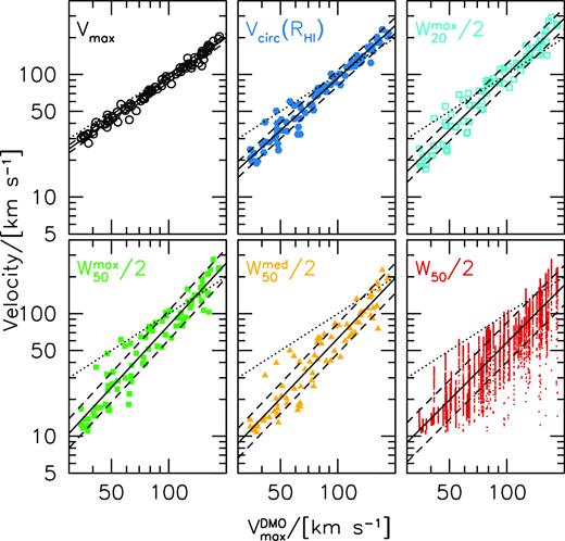
From maximum halo velocity |${V_{\rm max}^{\rm DMO}}$| to projected linewidth W50/2 for the full sample. Each panel shows a velocity versus |${V_{\rm max}^{\rm DMO}}$| relation. A fit to each relation of the form y = a + b(x − x0) is shown with solid (mean) and dashed (standard deviation) lines. The parameters of the fits are given in Table 1. For reference, the one-to-one line is shown with a dotted line. We see that the slope and scatter get progressively larger as we go from top left to bottom right.
Linear fits of the form y = a + b(x − x0) to various scaling relations. For all relations x0 is chosen to equal the mean of x. The scatter of the data about the model is σy.
| Sample | y | x | x0 | a | b | σy | Fig. |
|---|---|---|---|---|---|---|---|
| NIHAO | |$\log _{10}(W_{50}/2[{{ {\rm km\, s^{-1}} }}])$| | |$\log _{10}(V_{\rm max}^{\rm DMO}/[{{ {\rm km\, s^{-1}} }}])$| | 1.904 | 1.614 | 1.557 | 0.161 | 3 |
| NIHAO | |$\log _{10}(W_{20}/2[{{ {\rm km\, s^{-1}} }}])$| | |$\log _{10}(V_{\rm max}^{\rm DMO}/[{{ {\rm km\, s^{-1}} }}])$| | 1.904 | 1.751 | 1.419 | 0.120 | 3 |
| NIHAO | |$\log _{10}(V_{\rm max}/[{{ {\rm km\, s^{-1}} }}])$| | |$\log _{10}(V_{\rm max}^{\rm DMO}/[{{ {\rm km\, s^{-1}} }}])$| | 1.904 | 1.863 | 1.101 | 0.032 | 4 |
| NIHAO | |$\log _{10}(V_{\rm HI}/[{{ {\rm km\, s^{-1}} }}])$| | |$\log _{10}(V_{\rm max}^{\rm DMO}/[{{ {\rm km\, s^{-1}} }}])$| | 1.904 | 1.833 | 1.426 | 0.064 | 4 |
| NIHAO | |$\log _{10}(W_{20}^{\rm max}/2[{{ {\rm km\, s^{-1}} }}])$| | |$\log _{10}(V_{\rm max}^{\rm DMO}/[{{ {\rm km\, s^{-1}} }}])$| | 1.904 | 1.855 | 1.518 | 0.086 | 4 |
| NIHAO | |$\log _{10}(W_{50}^{\rm max}/2[{{ {\rm km\, s^{-1}} }}])$| | |$\log _{10}(V_{\rm max}^{\rm DMO}/[{{ {\rm km\, s^{-1}} }}])$| | 1.904 | 1.742 | 1.685 | 0.119 | 4 |
| NIHAO | |$\log _{10}(W_{50}^{\rm med}/2[{{ {\rm km\, s^{-1}} }}])$| | |$\log _{10}(V_{\rm max}^{\rm DMO}/[{{ {\rm km\, s^{-1}} }}])$| | 1.904 | 1.640 | 1.635 | 0.122 | 4 |
| SPARC | |$\log _{10}(R_1/[\rm kpc])$| | log10(Mstar/M⊙) | 9.493 | 1.109 | 0.281 | 0.18 | 15 |
| NIHAO | |$\log _{10}(R_1/[\rm kpc])$| | log10(Mstar/M⊙) | 8.325 | 0.779 | 0.303 | 0.24 | 15 |
| SPARC | |$\log _{10}(R_{\rm last}/[\rm kpc])$| | log10(Mstar/M⊙) | 9.471 | 1.109 | 0.311 | 0.23 | 15 |
| NIHAO | |$\log _{10}(R_{90}/[\rm kpc])$| | log10(Mstar/M⊙) | 8.309 | 0.789 | 0.252 | 0.23 | 15 |
| SPARC | Vslope | log10(Mstar/M⊙) | 9.471 | 0.123 | -0.137 | 0.19 | 16 |
| NIHAO | Vslope | log10(Mstar/M⊙) | 8.394 | 0.286 | -0.098 | 0.14 | 16 |
| SPARC | Vslope | |$\log _{10}(R_{\rm last}/[\rm kpc])$| | 1.109 | 0.123 | -0.399 | 0.18 | 16 |
| NIHAO | Vslope | |$\log _{10}(R_{90}/[\rm kpc])$| | 0.826 | 0.286 | -0.332 | 0.15 | 16 |
| NIHAO | (b/a)H i | log10(MH i/M⊙) | 8.83 | 0.585 | -0.013 | 0.20 | 17 |
There are a number of physical processes that play a role in the conversion of maximum circular velocity into projected H i linewidths: inflows and outflows; H i extent and rotation curve shape; non-circular motions, and projection. These are related, but not uniquely, to four ratios, which we show in Fig. 5.
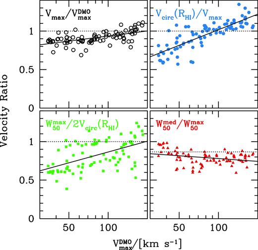
From |$V_{\rm max}^{\rm DMO}$| to projected linewidth W50 for the full sample using four independent ratios. Upper left shows |$V_{\rm max}/{V_{\rm max}^{\rm DMO}}$|, the ratio between the circular velocities of the hydro and DMO simulation at |$R_{\rm max}^{\rm DMO}$|. This is sensitive to mass in and outflows. The ratio varies from 0.8 to 1.1. Low-velocity haloes have ratios less than unity indicating mass-loss from the system. Upper right shows VHI/Vmax, the ratio between the circular velocity at the H i radius and the circular velocity at |$R_{\rm max}^{\rm DMO}$|. This ratio is sensitive to the shape of the circular velocity profile at the H i radius. The ratio varies from 0.6 to 1.3. High-velocity haloes have ratios greater than unity indicating declining velocity profiles, while low-mass haloes have ratios less than unity indicating rising velocity profiles. The lower left panel shows |$W_{50}^{\rm max}/2 V_{\rm H\,{\small I}}$|, the ratio between the maximum half linewidth and the circular velocity. This is sensitive to non-circular motions and the shape of the rotation curve. This ratio shows the largest variation from 0.4 to 1.2. The lower right panel shows |$W_{50}^{\rm med}/W_{50}^{\rm max}$|, the ratio between the median and maximum linewidths. This ratio is sensitive to the effects of projection and indicates whether galaxies behave like thin rotating discs (dotted line). The ratio varies from 0.6 to 1.0.
3.1 Inflows and outflows
The upper left panel shows |${V_{\rm max}}/{V_{\rm max}^{\rm DMO}}$|, which depends on the net inflow and outflow of baryons. At low velocities the ratio ≃0.85 indicating net outflows, while at high velocities the ratio is greater than 1, indicating net inflow. As a reference, if a system lost or did not accrete any of its baryons we would naively expect the ratio of |$\sqrt{(}1-f_{\rm bar})\simeq 0.92$|, where the cosmic baryon fraction, fbar = Ωb/Ωm ≃ 0.15. However, the reduction in halo velocity is larger than this because the loss of baryons at early times (as a result of the stellar feedback) reduces the accretion rate of dark matter, and hence the halo mass and maximum velocity of the halo by redshift |$z$| = 0. Similar results are seem in other cosmological hydrodynamical simulations, (e.g. Sawala et al. 2016), so the effect appears unrelated to the details of the sub-grid model for star formation and feedback.
3.2 H i extent and rotation curve shape
The upper right panel shows the VHI/Vmax ratio versus |${V_{\rm max}^{\rm DMO}}$|. In all galaxies VH i is measured at a smaller radius than Vmax, so the ratio depends on the shape of the circular velocity profile, and the extent of the H i gas. In high-velocity haloes the ratio is greater than 1 because the inflow of baryons. In low-mass haloes the ratio is less than 1 because the H i does not extend to the flat part of the velocity profile. At a halo velocity of 50 km s−1 the average ratio is 0.8, but there are some dwarf galaxies with a ratio of unity and others with a ratio of 0.6. This is already pointing to diversity of H i extent and/or rotation curve shapes.
3.3 Non-circular motions
The lower left panel shows the |$W_{50}^{\rm max}/2 {V_{\rm H\,{\small I}}}$| ratio. The linewidth is a convolution of the rotation curve with the H i distribution. In galaxies that are rotationally supported with a flat rotation curve this ratio is close to unity. When the ratio is less than unity this signals a rising rotation curve and/or significant non-circular motions. These can be dispersion in the gas, but also non-axisymmetric features such as bars, spiral arms, and warps, and out of equilibrium gas flows due to e.g. SN-driven winds or mergers. At a halo velocity of 50 km s−1 the average ratio is 0.7, but again there is significant scatter, with some dwarf galaxies with a ratio close to unity.
3.4 Projection
The lower right panel shows the ratio between the median and maximum W50 linewidth. This ratio tells us about projection effects. The inclination angle, i, where i = 0 is face-on, and i = 90 is edge-on, is distributed uniformly in cos (i) from 0 to 1. For a thin rotating disc with negligible velocity dispersion, the linewidth at inclination, i, is related to the linewidth at inclination i = 90 by Wi = sin (i)W90. The ratio between the median linewidth (i = 60) and the maximum (i = 90) is thus sin (60) = 0.866. In the figure we see a few galaxies at all halo velocities near this value (dotted line). However, the majority of galaxies lie below this line indicating the galaxies are in general not thin rotating discs. This is another manifestation of the role of non-circular motions. At a halo velocity of 50 |${{ {\rm km\, s^{-1}} }}$| the average ratio is 0.8. At the lowest velocities the ratio is close to unity, indicating these systems (or at least the H i lines) have very little rotational support.
4 IMPLIED VELOCITY FUNCTIONS
We now discuss how the various velocity definitions result in velocity functions with different slopes. First we show results with power laws, as the transformations are simple and analytic. Then we consider the impact of Gaussian scatter, and finally the actual distribution of linewidths from our simulations corresponding to non-power laws and non-Gaussian scatter.
4.1 Analytic considerations for the velocity function
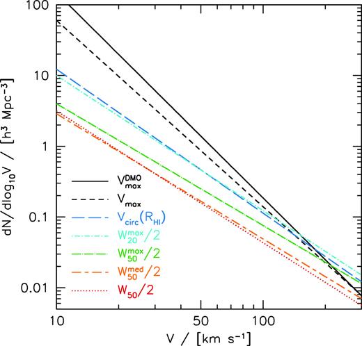
Velocity functions based on different velocity definitions calculated using the fitting formula in Fig. 3. The slopes get progressively shallower as we go from maximum dark halo velocity |${V_{\rm max}^{\rm DMO}}$| to H i half-linewidth W50/2.
Velocity functions for NIHAO simulations from Fig. 6 of the form |$\mathrm{ d}N/\mathrm{ d}\log _{10}V = A (V/[50\,{{ {\rm km\, s^{-1}} }}])^{\alpha }$|.
| Definition | α | A |
|---|---|---|
| |$V_{\rm max}^{\rm DMO}$| | −2.90 | 30641.38 |
| Vmax | −2.63 | 0.867 |
| VH i | −2.03 | 0.464 |
| |$W_{20}^{\rm max}/2$| | −1.91 | 0.462 |
| |$W_{50}^{\rm max}/2$| | −1.72 | 0.249 |
| |$W_{50}^{\rm med}/2$| | −1.77 | 0.166 |
| W50/2 | −1.80 | 0.158 |
| Definition | α | A |
|---|---|---|
| |$V_{\rm max}^{\rm DMO}$| | −2.90 | 30641.38 |
| Vmax | −2.63 | 0.867 |
| VH i | −2.03 | 0.464 |
| |$W_{20}^{\rm max}/2$| | −1.91 | 0.462 |
| |$W_{50}^{\rm max}/2$| | −1.72 | 0.249 |
| |$W_{50}^{\rm med}/2$| | −1.77 | 0.166 |
| W50/2 | −1.80 | 0.158 |
4.2 Impact of Gaussian scatter
Fig. 7 shows the impact of Gaussian (in log(V)) scatter on the velocity function. The black line shows the velocity function using |${V_{\rm max}^{\rm DMO}}$|, sampled between a velocity of 30–200 |${{ {\rm km\, s^{-1}} }}$|. The red dotted line shows the velocity function using W50/2. The other lines show the impact of lognormal scatter (0.1, 0.2, and 0.3 dex) in the relation between W50/2 and |${V_{\rm max}^{\rm DMO}}$|. The effect of scatter is to increase the normalization of the velocity function. Galaxies get preferentially scattered to higher velocity because there are many more low-velocity haloes than high-velocity haloes. The overall effect is not large, just 0.1 dex change for a scatter of 0.2 dex.
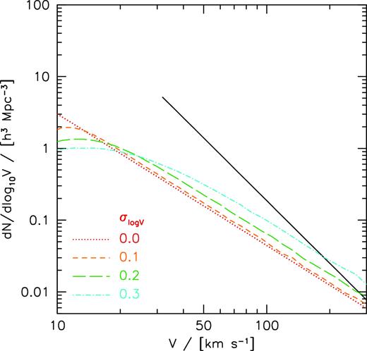
Effect of scatter on the velocity function. Starting from the W50/2 velocity function (red dotted line) we add lognormal scatter of magnitude 0.1 (orange), 0.2 (green), and 0.3 (cyan). Low-velocity galaxies get preferentially scattered to high velocities, thereby increasing the normalization of the velocity function. For reference the black line shows the |${V_{\rm max}^{\rm DMO}}$| function.
4.3 Deriving the velocity function from linewidth versus maximum circular velocity
As fiducial bin widths we adopt dx = 0.05 and dy = 0.10. The resulting velocity functions for W50 (left) and W20 (right) are shown with red points in Fig. 8, and tabulated in Table 3. The error bars (ey) are calculated as |$e_y=y/\sqrt{N}$|, where N is the number of simulations that contribute to each y-bin. At low velocities (|$W_{50}/2 \lt 80\, {{ {\rm km\, s^{-1}} }}$|) the NIHAO W50/2 function has a normalization and shallow slope ∼−1 in agreement with observations from the Local Volume (Klypin et al. 2015) and ALFALFA (Papastergis & Shankar 2016). At high velocities (|${\gtrsim}100 \,{{ {\rm km\, s^{-1}} }}$|) the NIHAO simulations underpredict the observed number densities, or alternatively the linewidths are too low. We return to a possible cause of this in Section 5.3 below.
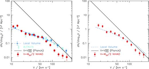
Linewidth velocity function derived from the full distribution of linewidths and |${V_{\rm max}^{\rm DMO}}$| in the NIHAO simulations (red points) using W50/2 (left) and W20/2 (right). The black solid lines show the CDM halo (|${V_{\rm max}^{\rm DMO}}$|) velocity function, which has a steep slope of −2.9. Observational data from the Local Volume and ALFALFA using W50 are shown with blue and cyan circles, respectively. The blue dashed line shows the fit to the Local Volume from Klypin et al. (2015). In the right-hand panel we transform the observations using the approximation |$W_{20}=W_{50}+25\, {{ {\rm km\, s^{-1}} }}$|, with a minimum W50/W20 = 0.63.
Differential velocity functions for NIHAO simulations from Fig. 8.
| log (V) | dN/dlog (V) | Error | dN/dlog (V) | Error |
|---|---|---|---|---|
| W50/2 | W20/2 | |||
| 1.05 | 1.559 | 0.332 | – | – |
| 1.15 | 1.747 | 0.295 | – | – |
| 1.25 | 0.743 | 0.116 | 1.888 | 0.385 |
| 1.35 | 0.469 | 0.072 | 1.603 | 0.271 |
| 1.45 | 0.413 | 0.061 | 0.617 | 0.095 |
| 1.55 | 0.398 | 0.061 | 0.671 | 0.107 |
| 1.65 | 0.289 | 0.044 | 0.500 | 0.078 |
| 1.75 | 0.270 | 0.039 | 0.378 | 0.058 |
| 1.85 | 0.138 | 0.021 | 0.233 | 0.036 |
| 1.95 | 0.0747 | 0.0128 | 0.134 | 0.021 |
| 2.05 | 0.0308 | 0.0060 | 0.0781 | 0.0136 |
| 2.15 | 0.0163 | 0.0040 | 0.0330 | 0.0069 |
| 2.25 | 0.0130 | 0.0041 | 0.0195 | 0.0050 |
| 2.35 | 0.0105 | 0.0043 | 0.0154 | 0.0054 |
In our simulations W20/2 is a better predictor of the halo velocity than W50/2 (see Fig. 4) so this is our preferred definition for future observations. Currently observations of the W20 function are not available, so we shift the observations using the approximation |$W_{20}=W_{50}+25\, {{ {\rm km\, s^{-1}} }}$| (Brook, Santos-Santos & Stinson 2016), and a minimum of W50/W20 = 0.63. In this case the simulations are closer to the observed velocity function at high velocities, while maintaining the agreement at low velocities.
5 TESTING THE SIMULATIONS
We have shown that the discrepancy at low velocities between the observed H i linewidth function and the |${V_{\rm max}^{\rm DMO}}$| function of LCDM is resolved by the NIHAO simulations. We now discuss in more detail why this is the case, and observational ways in which the simulations can be tested. We focus our discussion on six (mostly dimensionless) parameters that are correlated with the variation in H i linewidth at fixed maximum dark halo velocity.
Rotation-to-dispersion ratio, Vrot/σH i. The H i dispersion is calculated from the minimum H i linewidth, |$\sigma _{\rm H\,{\small I}}=W_{50}^{\rm min}/2.35$|. For the rotation velocity we use the maximum of the rotation curve, which tends to occur near the H i radius (see Fig. 1 for examples). This definition is not directly observable, but similar definitions are.
γ1, Skewness of the W50 distribution, see below for definition. Can be measured on samples of galaxies.
H i line profile shape, W50/W20. Directly observable.
Outer circular velocity curve slope, Δlog V/Δlog R. For our simulations is measured between 0.5 and 1.0 RH i. Can be measured for individual galaxies.
H i-to-virial radius, RHI/R200. Dimensionless, but not directly observable. H i sizes are observable.
H i disc thickness. Computed as the minimum H i axis ratio from all projections. Can be measured from samples of galaxies.
5.1 Testing rotational support with projection effects
One of the key results from our simulations is that galaxies, and dwarf galaxies in particular, do not always have H i kinematics as expected from idealized thin rotating discs. An observationally testable consequence of this is the effect of projection.
For a thin rotationally supported axisymmetric disc the minor-to-major axis ratio (b/a) is uniformly distributed between 0 and 1. In terms of the disc inclination, i, where i = 0 is face-on and i = 90 is edge-on, b/a = cos (i), the observed linewidth then varies as sin (i). Fig. 9 shows the linewidth versus axis ratio for our four test galaxies. The axis ratio is computed for each projection using moments as described in Section 2. The upper galaxies have maximum halo velocity |${V_{\rm max}^{\rm DMO}}\simeq 55 {{ {\rm km\, s^{-1}} }}$|, while the lower two galaxies have |${V_{\rm max}^{\rm DMO}}\sim 100 {{ {\rm km\, s^{-1}} }}$|. The corresponding stellar masses are ∼2 × 10⁸ and ∼109 M⊙, respectively.
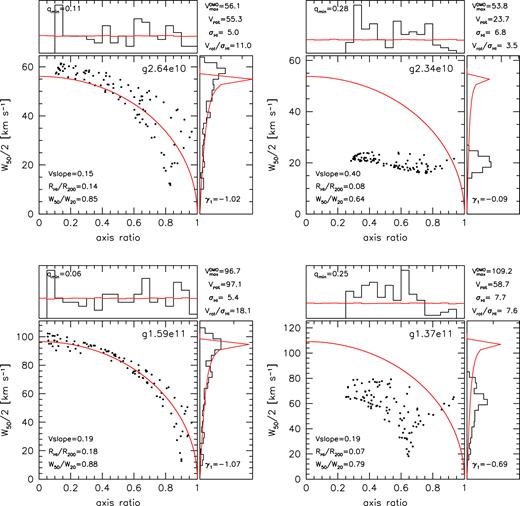
Projection effects in the linewidth versus axis ratio plane for four test galaxies. Upper panels show galaxies with maximum circular velocity |${V_{\rm max}^{\rm DMO}}\sim 55\, {{ {\rm km\, s^{-1}} }}$|, while lower panels show galaxies with |${V_{\rm max}^{\rm DMO}}\sim 100\, {{ {\rm km\, s^{-1}} }}$|. Left-hand panels show rotation dominated galaxies, right-hand panels show galaxies with more pressure support, as can be seen by the thicker H i discs (qmin), and more symmetric distributions of linewidths (γ1). The red lines show the prediction for a randomly oriented thin disc rotating at (|${V_{\rm max}^{\rm DMO}}$|) – uniform axis ratios, and linewidths scaling as sin (i), where cos (i) is uniformly distributed.
The two galaxies on the left-hand panels of Fig. 9 have close to uniform axis ratio distributions (upper histograms) and strongly skewed linewidth distributions (right histograms) close to that predicted for thin discs rotating at the maximum velocity of the dark matter halo (solid red lines). On the other hand, the two galaxies in the right-hand panels of Fig. 9 strongly deviate from this prediction with a lower mean linewidths and a more symmetric distribution of linewidths. The axis ratio distribution is also more centrally concentrated.
The galaxies in the left-hand panels of Fig. 9 have γ1 = −0.97 and −1.06, i.e. they behave like thin rotating discs. In contrast the galaxies on the right have γ1 = −0.10 and γ1 = −0.73, and are thus less rotationally supported systems. These inferences agree with the actual rotation to dispersion ratios (Vrot/σH i).
Another parameter that is related to the rotational support of a galaxy is minimum minor-to-major axia ratio, qmin (i.e. the disc thickness). The galaxies on the left have smaller minimum axis ratios (corresponding to thinner edge-on discs): qmin = 0.11 and 0.06 compared to 0.28 and 0.25.
The ratio between linewidths W50/W20, also depends on the rotational support, as well as the circular velocity curve shape, and the extent of the H i. The galaxies on the left have steeper line profiles, and more extended and shallower outer circular velocity curve slopes.
5.2 What causes linewidths to underestimate maximum circular velocity?
Fig. 10 shows the impact of several (mostly dimensionless) parameters on the relation between median H i linewidth and maximum dark halo circular velocity. The points are colour coded by the parameter in question. The four numbers in each panel indicate the mean value of each quartile, the solid line is a fit to each quartile of points. We discuss each of them in turn below.
Outer circular velocity curve slope (top left). A positive value indicates that the curve is still rising in the outer parts, while a value close to zero indicates a flat velocity curve. Galaxies with more rising circular velocity profiles (red points) tend to have lower linewidth-to-halo velocity ratios.
H i-to-virial radius (top middle). Smaller galaxies (blue triangles) have lower linewidths. At least partially because if the H i does not reach the flat part of the circular velocity curve, then the kinematics will progressively underestimate the maximum circular velocity.
H i axis ratio (top right). The thinnest galaxies (red points, b/a ∼ 0.1) have linewidths that trace the halo velocity, while thicker galaxies have progressively lower linewidths.
γ1, Skewness of the W50 distribution (top left). Galaxies with strong negative skew (blue points) have linewidths that trace the maximum halo velocity. Larger values of γ1 result in lower linewidths.
Rotation-to-dispersion ratio (bottom middle). Rotationally supported systems (red circles) tend to have linewidths that trace the halo velocity, while pressure supported systems (blue triangles) tend to have low linewidths.
H i line profile shape (bottom left). Steeper line profiles W50/W20 ∼ 0.9 (red points) have linewidths close to halo velocity, while shallow line profiles W50/W20 ∼ 0.6 (blue triangles) have linewidths significantly below the halo velocity. The profile shape depends on a combination of the rotation curve shape and extent, and the rotation to dispersion ratio.
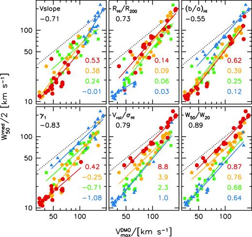
Relation between median H i linewidth and maximum circular velocity of the dark matter halo. Points are colour coded by the parameter indicated in the top left corner of each panel. The number at the top left corner is the correlation coefficient between said parameter and |$W_{50}^{\mathrm{ med}}/2$| and |${V_{\rm max}^{\rm DMO}}$|. Structural parameters: logarithmic slope of the outer circular velocity profile (top left); H i-to-virial radius (top middle); minimum minor-to-major H i axis ratio (top right). Kinematic parameters: skewness of the linewidth distribution (bottom left); rotation-to-dispersion ratio (bottom middle); and linewidth profile shape (bottom right). Each colour corresponds to a quartile of the distribution (red are the largest 25 per cent, while blue are the smallest 25 per cent), the mean of each quartile is indicated by the coloured numbers.
The number in the top left indicates the correlation coefficient between the specific parameter and |$W_{50}^{\rm med}/2 {V_{\rm max}^{\rm DMO}}$|. Line profile shape shows the strongest correlation (ρ = 0.89) closely followed by the skewness (ρ = −0.83), and H i rotation to dispersion ratio (ρ = 0.79). At a given halo velocity all six parameters show a correlation with linewidth. To see which of these parameters is most likely to explain the trend with halo mass, we show the dependence on halo velocity in Fig. 11. The straight and dashed lines show a fit with 1σ scatter. The number gives the correlation coefficient. We see clear trends but also significant scatter. Structurally, we see that lower velocity haloes have steeper outer circular velocity curve slopes and relatively smaller H i sizes, and marginally thicker H i discs. Kinematically, we see that lower velocity haloes have less negatively skewed H i linewidth distributions, lower rotation-to-dispersion ratios, and shallower line profiles.
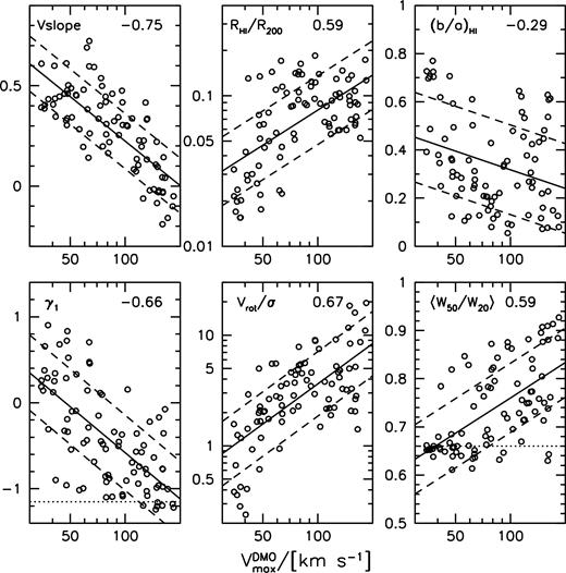
Parameters versus halo velocity. The parameter in question is indicated in the top left corner. The correlation coefficient is given in the top right corner. The mean and standard deviation of a linear fit is shown with sold and dashed lines. Dotted horizontal lines indicate the expectation for a rotating disc (lower left) and Gaussian (lower right).
In summary we see that the dependence of W50 with |${V_{\rm max}^{\rm DMO}}$| is driven primarily by two effects: the degree of rotational support and the shape of the rotation curve. Galaxies in lower mass haloes have less rotational support, and less extended H i. Below we show current observations that show evidence of these two effects.
5.3 Line profile shape
The shape of the H i line profile depends on the amount of rotational support and the shape of the rotation curve. A simple way to parametrize this is the ratio between linewidths measured at the 50 per cent and 20 per cent level of peak flux, W50 and W20. The ratio is close to 1 for a rotating disc with a flat rotation curve whose velocity dispersion is small compared to the line-of-sight component of the rotation velocity. As the outer rotation curve slope becomes more positive the ratio decreases, since a larger fraction of the H i flux is coming from gas rotating lower than the maximum. Pressure support also causes ratio to decrease. In the limit V/σ = 0 the line profile is simply that due to random motions of the gas, and is independent of the rotation curve shape. For a Gaussian |$W_{50}/W_{20}=\sqrt{\ln (0.5)/\ln (0.2)}\simeq 0.66$|. The observational advantage of this ratio is it does not require spatially resolved H i observations, which are currently not feasible for large samples of galaxies.
A comparison between NIHAO simulations and observations was previously shown in Macciò et al. (2016). In both observations and simulations the W50/W20 decreases for lower linewidth galaxies. This result was also shown by Brook et al. (2016) using a smaller sample of galaxies from the MaGICC project (the precursor to NIHAO), and by El-Badry et al. (2018) using galaxies from the FIRE project.
Fig. 12 shows the relation between W50 and W20 from NIHAO simulations compared to observations from HIPASS (Koribalski et al. 2004) and THINGS (Walter et al. 2008). In both simulations and observations the ratio varies from ∼0.95 at high velocities to ∼0.65 at low velocities, and the amount of scatter is also similar. However, when looking at the median relations (lower right panel) the NIHAO simulations underpredict the HIPASS observations for |$W_{50}\sim 100 \,{{ {\rm km\, s^{-1}} }}$|. This is the same scale where the simulations underpredict the observed velocity function (Fig. 8). The upper right panel shows the distributions of W50/W20 in five bins of W50/2. Again this shows an excess of galaxies in NIHAO with low linewidth ratios at intermediate velocities. In principle this could be due to there being too much non-circular motions and/or the H i discs being too small at this velocity scale. Since the NIHAO simulations are in good agreement with observations of H i sizes (see below), we think the low linewidth ratio is more likely due to too an excess of non-circular motions, likely driven by feedback. Due to the large intrinsic variation in W50/W20 and the relatively small sample size, another contributing cause could be sampling effects, i.e. we by chance happen to simulate more galaxies with lower ratios. A similar discrepancy in W50/W20 at this velocity scale is seen in the FIRE simulations (El-Badry et al. 2018) and likely has a common origin, which points to feedback driven turbulence.
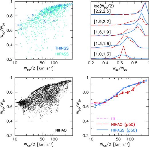
Linewidth ratio W50/W20 versus W50/2. NIHAO simulations are shown with black points (100 projections per galaxy) and red long -dashed lines. HIPASS observations are shown with cyan points and blue solid lines. THINGS observations are shown with blue circles. The left-hand panels show the distribution of points, the lower right panel shows the median relations, where the error bars show the error on the median. For NIHAO this is the error corresponding to the number of distinct galaxies in each bin, rather than the number of data points (which is ∼30 times higher). The dashed magenta line is a simple fit to the observations: |$W_{20}=W_{50} +25 \, {{ {\rm km\, s^{-1}} }}$| with a minimum of 0.64. The upper right panel shows the distribution of W50/W20 in five bins of W50/2 as indicated.
In summary, the H i line profile shape is a powerful, yet simple test of the simulations, and thus motivates future blind H i surveys obtaining deep enough data to accurately measure both W50 and W20.
5.4 Skewness of the linewidth distribution
For observed galaxies we only get a single projection per galaxy. However, for a sample of galaxies, we can expect a random distribution of projections, provided we select galaxies by a parameter that is independent of the projection angle, such as the H i mass.
Fig. 13 shows the distributions of H i linewidth versus H i mass. Single dish observations are from the ALFALFA survey (Haynes et al. 2018) and HIPASS (Koribalski et al. 2004). The lower right panel shows the dependence of γ1 measured in bins of H i mass. The two observational datasets and simulations find consistent results, for the skewness of both W50 (solid lines) and W20 (dashed lines). Namely high-mass galaxies are strongly negatively skewed, close to the value expected for thin rotating discs. Lower mass galaxies have higher γ1. This is an observational signature that lower mass galaxies are more kinematically disordered. For the lowest mass galaxies the distribution of linewidths is positively skewed, which is a signature of a floor in the linewidth from thermal broadening of the H i line.
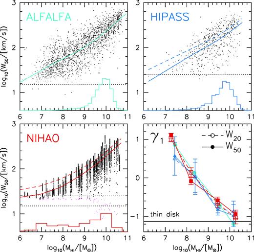
The H i linewidth–mass relation. Upper panels show the observed relations from ALFALFA and HIPASS. Points are W50, solid lines show the mean relation. Dashed lines show the mean relation using W20. Only 100 points per 0.2 dex in mass are plotted to make the change in scatter with mass more apparent. The histogram shows the distribution of mass for the full sample. The horizontal dotted lines show the instrumental velocity resolution limit. The lower left panel shows the relation from NIHAO, where we plot 50 random projections per simulated galaxy. The magenta points show the linewidth due to thermal broadening. The lower right panel shows the skewness of the distribution in bins of mass. Error bars are from bootstrap resampling. An idealized thin rotating disc has γ1 = −1.13 (horizontal black line). High-mass galaxies in both observations and simulations are close to this value. While lower mass galaxies progressively deviate suggesting more disordered kinematics.
The distribution of linewidths in bins of H i mass can also be used to estimate the velocity dispersion of the H i gas, σH i. This is because for a galaxy disc that is face-on, there will be zero rotational component projected into the line of sight, and thus the observed linewidth will be a reflection of the disordered motions of the gas. Assuming the line profiles are Gaussian σHI = W50/2.355. The minimum linewidth is subject to observational measurement errors, and may not be representative of the population, so we take the average of the lowest 5 per cent of linewidths. This will give an upper limit to σH i because for a thin rotating disc the lowest 5 per cent of inclinations result in a line-of-sight rotation that is |${\sim }23{{\ \rm per\ cent}}$| of the edge-on value.
The results of this exercise are shown with the solid points in Fig. 14. Overall there is good agreement between the observations and simulations. In detail there are some differences. Comparing the observations, in the low-mass bins HIPASS results in |${\sim } 3\,{{ {\rm km\, s^{-1}} }}$| higher σHI than ALFALFA, likely due to the lower spectral resolution of HIPASS (indicated with horizontal lines). Except for the highest mass bin, the NIHAO simulations have slightly higher σH i than ALFALFA. For NIHAO the red open squares show the thermal velocity dispersion. The difference between the solid red and open red points is thus the contribution of turbulence (and projected rotation). Since projection affects both simulations and observations the slightly higher dispersions in NIHAO are thus caused by turbulence, likely as a result of the feedback being too strong.
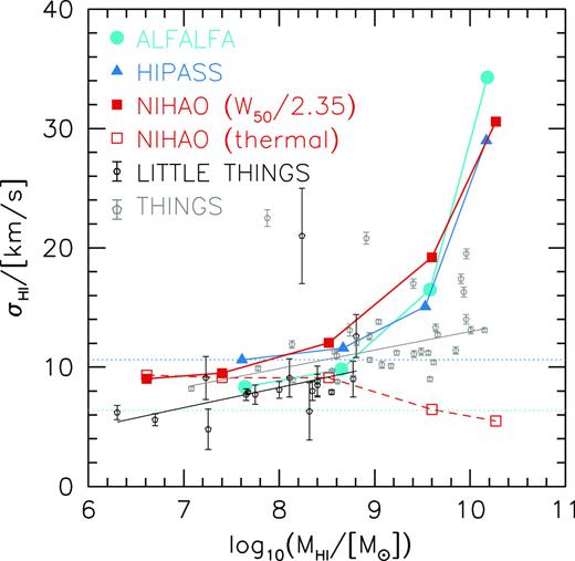
H i velocity dispersion versus H i mass. For NIHAO (red), ALFALFA (cyan), and HIPASS (blue) the velocity dispersion is estimated from the ‘face-on’ linewidths using σH i = 〈W50〉/2.35, where 〈W50〉 is the average of the lowest 5 per cent of linewidths in a given bin of H i mass. For thin rotating discs, this includes a non-negligible contribution from rotation, so should be considered an upper limit to σH i. For NIHAO the open squares show the average of the thermal velocity dispersion. The horizontal dotted lines show the resolution limits of ALFALFA (cyan) and HIPASS (blue), and suggest that the HIPASS dispersions are effected by the resolution limit. Measurements for individual galaxies using resolved H i observations from LITTLE THINGS (Iorio et al. 2017) and THINGS (Ianjamasimanana et al. 2012) are shown with black and grey points with error bars, respectively. The lines show fits to these data.
The black and grey points show measurements from individual galaxies using spatially resolved H i observations from THINGS (Ianjamasimanana et al. 2012) and LITTLE THINGS (Iorio et al. 2017). The solid lines show linear fits with 3σ clipping. The slopes are similar, but there is a small offset of |${\simeq } 2 {{ {\rm km\, s^{-1}} }}$|, likely reflecting a systematic in the measurement techniques. In the mass range 107 M⊙ < MH i < 109 M⊙ the resolved measurements are in good agreement with the spatially unresolved linewidth based measurements. Thus in the future our technique can be used to infer the velocity dispersions of large samples of spatially unresolved observations. At higher masses (MH i > 109 M⊙) the resolved measurements give lower dispersions than the unresolved measurements. As mentioned above, projected rotation likely contributes to this difference. In addition, the linewidth based dispersion includes deviations from a perfectly axisymmetric disc. For example, a warp will prevent the projected rotation from being zero at any viewing angle, increasing the implied dispersion. Another possible contributing effect is the role of sample selection. The THINGS survey is not a complete sample of galaxies, it is possibly biased towards that more rotation dominated galaxies at these masses than the galaxy population.
In summary, the distribution of linewidths in bins of Hi mass shows that in both simulations and observations lower mass galaxies are less rotationally supported than more massive galaxies. This is driven by a reduction in the rotation velocity in low-mass galaxies rather than an increase in the gas dispersion, which also decreases in lower mass galaxies.
5.5 H i sizes
We showed previously in Macciò et al. (2016) that the NIHAO galaxies match two H i size versus H i mass relations (the exponential scale length, and the radius where the surface density reaches 1 M⊙ pc−2). We are interested in the relation between H i size and halo mass, but halo masses are not directly observable. In the NIHAO simulations, stellar mass is the galaxy observable that is most strongly correlated with halo mass (correlation coefficient of 0.98). The scatter in the stellar mass versus halo mass relation is small (∼0.2 dex) both in theory (Dutton et al. 2017; Matthee et al. 2017), and observations (More et al. 2011; Reddick et al. 2013; Moster, Naab & White 2018). Here we use galaxies from the SPARC survey (Lelli, McGaugh & Schombert 2016) as this is the largest compilation of resolved H i rotation curves with 3.6 |$\mu$|m Spitzer imaging (which gives the most reliable stellar mass tracer).
Fig. 15 shows H i size versus stellar mass relations and a comparison between various H i size definitions. The upper panels show that R1 (the radius where the H i surface density drops to 1 M⊙ pc−2) is closely related to R90 in the NIHAO simulations and Rlast in the SPARC observations. The lower left panel shows a very good agreement between the R1 versus stellar mass relations in NIHAO (red) and SPARC (blue). Fits to the size–mass relations are given in Table 1.
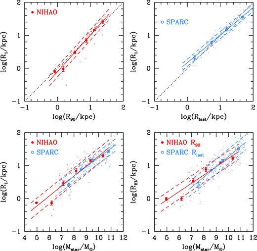
H i size versus stellar mass relation. In the NIHAO simulations (red points) sizes enclose 90 per cent of the H i mass from a face-on projection. In the SPARC observations (blue points) sizes are the last point on the H i rotation curve. Points show individual galaxies, circles show mean sizes in bins of H i mass, the error bar shows the error on the mean, and solid and dashed lines show a linear fit and its standard deviation.
While the observations are not a complete sample of nearby galaxies the comparison is a good place to start. It contradicts the claim by Trujillo-Gomez et al. (2018) that the H i distribution in NIHAO galaxies is too compact compared to observations. This was suggested by Trujillo-Gomez et al. (2018) as a reason for the low |$W_{50}/2{V_{\rm max}^{\rm DMO}}$| ratio in NIHAO dwarf galaxies. As shown in Fig. 11, the H i in NIHAO dwarf galaxies is less extended relative to the dark matter halo than in more massive galaxies. So this does contribute to the low |$W_{50}/2{V_{\rm max}^{\rm DMO}}$| ratios in dwarfs. However, rather than being an artefact of NIHAO, this appears to be a feature of real galaxies.
5.6 Outer H i rotation curve slopes
Fig. 16 shows the logarithmic slope (Δlog V/Δlog R) of the outer rotation curve versus the stellar mass (left) and the H i radius (right). Points show individual galaxies, while symbols with error bars show the mean and error on the mean in bins of mass or radius. For the observations the slope is measured between 0.5 and 1.0 Rlast on the rotation curve, for the simulations the fiducial slope is measured between 0.5 and 1.0 RH i on the circular velocity curve (red filled circles), and on the rotation curve (pink open circles).
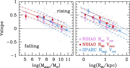
Logarithmic slope of the outer velocity curve versus stellar mass (left) and H i radius (right). In the NIHAO simulations the slope is measured between 0.5 and 1.0 RH i on the circular velocity curve (red) and the rotation velocity curve (pink). For the observations from SPARC (blue) the slope is measured between 0.5 and 1.0 Rlast on the rotation curve. This shows that in both simulations and observations lower mass and smaller galaxies have more strongly rising velocity curves.
The simulations are in good agreement with the observations, except that the observed relations have slightly larger scatter, plausibly due to larger measurement errors. We see that high mass or large galaxies have, on average, flat outer rotation curves at the H i radius. As we go to lower stellar masses and smaller sizes the outer rotation curves are progressively rising. Notice that even though both observations and simulations include cored dark matter density profiles in dwarf galaxies, at large radii the typical outer rotation curve slope is ∼0.5 corresponding to a ρ ∝ r−1 density profile. When the rotation curve is rising, the half-linewidth W50/2 will necessarily underestimate the maximum rotation velocity.
5.7 Axis ratios
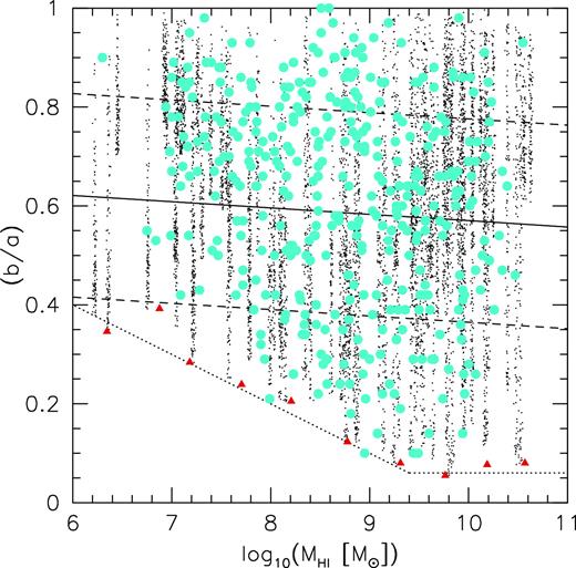
Dependence of projected H i axis ratio on H i mass. For NIHAO simulations each galaxy has 100 projections shown (black points). The red triangles show the minimum axis ratio in bins of mass showing a deficit of small axis ratios in low-mass galaxies. This is consistent with observations (cyan circles) from Wang et al. (2016).
The cyan circles show observed galaxies from the nearby Universe from Wang et al. (2016). This study combines H i data from several different projects so is representative of a wide variety of galaxy types and environments: Atlas3D (Serra et al. 2012, 2014), Bluedisk (Wang et al. 2013), and Faint Irregular Galaxies GMRT Survey (FIGGS) (Begum et al. 2008). LITTLE THINGS (Hunter et al. 2012), Local Volume H i Survey (LVHIS) (Koribalski et al. 2018), starbursting dwarf galaxies (Lelli, Verheijen & Fraternali 2014), The H i Nearby Galaxy Survey (THINGS) (Walter et al. 2008), Ursa Major cluster (Verheijen & Sancisi 2001), Void Galaxy Survey (VGS) (Kreckel et al. 2012), VLA Imaging of Virgo Spirals in Atomic Gas (VIVA) (Chung et al. 2009), and Westerbork H i survey of spiral and irregular galaxies (WHISP) (Swaters et al. 2002; Noordermeer et al. 2005).
For the vast majority of galaxies (88 per cent) the axis ratio is determined by Wang et al. (2016) from the H i maps, based on the second-order moments of the pixel distributions where ΣH i > 1 M⊙ pc−2. For the galaxies in VIVA (36) and Atlas3D (8) axis ratios are from tilted ring fits to the velocity fields. Galaxies that are poorly resolved (H i radius less than the beam major axis) have been excluded, though this does not guarantee the axis ratios are well resolved in all galaxies.
The observations and simulations have similar distributions of axis ratios, in particular there are no observed galaxies in the lower left corner where our simulations predict there to be none. This appears to confirm the lack of dwarf galaxies with thin H i discs. Future observations of a complete sample of galaxies with higher spatial resolution are needed to conclusively confirm the lack of thin dwarf galaxies.
6 SUMMARY
We use a sample of 85 galaxies simulated in an LCDM cosmology from the NIHAO project to investigate why H i linewidths systematically underpredict the maximum dark halo circular velocities in dwarf galaxies (Fig. 3). We trace this to two primary effects.
Lower mass galaxies are less rotationally supported. This is confirmed observationally from the skewness of linewidths in bins of H i mass in both ALFALFA and HIPASS observations (Fig. 13).
The H i distributions are less extended (relative to the dark matter halo) in dwarf galaxies, so that the rotation curves are still rising at the last measured data point, in agreement with observations (Fig. 16).
The H i profile shape parametrized by W50/W20 decreases in lower mass galaxies (Fig. 12) consistent with both these two effects. An additional observational test is in the distribution of H i axis ratios. In particular, in the NIHAO simulations the minimum axis ratio is larger in lower mass galaxies (Fig. 17).
In our simulations the H i kinematics are an inhomogeneous population. There is a significant range of rotational support and H i extent at any given halo or galaxy mass. This variation drives the variation in |$W_{50}/2{V_{\rm max}^{\rm DMO}}$| (Fig. 10). Thin and extended rotating H i discs exist in our simulations at all halo masses, but they are not a fair sample. This implies that one cannot use a sample of well-ordered rotating discs to interpret the H i linewidths of large unbiased samples of galaxies, as is sometimes done (e.g. Papastergis & Ponomareva 2017; Trujillo-Gomez et al. 2018).
The implied linewidth velocity function from the NIHAO simulations has a shallow slope (≃−1) at low velocities (|$10\, {{ {\rm km\, s^{-1}} }} \lt W_{50}/2 \lt 80\, {{ {\rm km\, s^{-1}} }}$|), consistent with observations (Fig. 8). Thus we conclude that the apparent discrepancy between the predictions of the LCDM cosmological model and observations as highlighted by previous authors (Papastergis et al. 2011; Klypin et al. 2015) is due to their incorrect assumption that |$W_{50}/2 \simeq {V_{\rm max}^{\rm DMO}}$|.
We look forward to the next generation of blind H i line surveys, APERTIF (Verheijen et al. 2008) and ASKAP (Johnston et al. 2008) that will provide higher spatial resolution data with which to further test our simulations and thus the LCDM model.
ACKNOWLEDGEMENTS
We thank the anonymous referee for a detailed and constructive report. This research was carried out on the High Performance Computing resources at New York University Abu Dhabi; on the theo cluster of the Max-Planck-Institut für Astronomie and on the hydra clusters at the Rechenzentrum in Garching. The authors gratefully acknowledge the Gauss Centre for Supercomputing (GCS) e.V. (www.gauss-centre.eu) for funding this project by providing computing time on the GCS Supercomputer SuperMUC at Leibniz Supercomputing Centre (http://www.lrz.de). AO is funded by the Deutsche Forschungsgemeinschaft (DFG, German Research Foundation) – MO 2979/1-1.
