


Abstract
In the past few years, several independent collaborations have presented cosmological constraints from tomographic cosmic shear analyses. These analyses differ in many aspects: the data sets, the shear and photometric redshift estimation algorithms, the theory model assumptions, and the inference pipelines. To assess the robustness of the existing cosmic shear results, we present in this paper a unified analysis of four of the recent cosmic shear surveys: the Deep Lens Survey (DLS), the Canada–France–Hawaii Telescope Lensing Survey (CFHTLenS), the Science Verification data from the Dark Energy Survey (DES-SV), and the 450 deg2 release of the Kilo-Degree Survey (KiDS-450). By using a unified pipeline, we show how the cosmological constraints are sensitive to the various details of the pipeline. We identify several analysis choices that can shift the cosmological constraints by a significant fraction of the uncertainties. For our fiducial analysis choice, considering a Gaussian covariance, conservative scale cuts, assuming no baryonic feedback contamination, identical cosmological parameter priors and intrinsic alignment treatments, we find the constraints (mean, 16 per cent and 84 per cent confidence intervals) on the parameter S8 ≡ σ8(Ωm/0.3)0.5 to be |$S_{8}=0.942_{-0.045}^{+0.046}$| (DLS), |$0.657_{-0.070}^{+0.071}$| (CFHTLenS), |$0.844_{-0.061}^{+0.062}$| (DES-SV), and |$0.755_{-0.049}^{+0.048}$| (KiDS-450). From the goodness-of-fit and the Bayesian evidence ratio, we determine that amongst the four surveys, the two more recent surveys, DES-SV and KiDS-450, have acceptable goodness of fit and are consistent with each other. The combined constraints are |$S_{8}=0.790^{+0.042}_{-0.041}$|, which is in good agreement with the first year of DES cosmic shear results and recent CMB constraints from the Planck satellite.
1 INTRODUCTION
The large-scale structure of the Universe bends the light rays emitted from distant galaxies according to General Relativity (Einstein 1936). This effect, known as weak (gravitational) lensing, introduces coherent distortions in galaxy shapes, which carry information of the cosmic composition and history.
Since the first detection of cosmic shear in Bacon, Refregier & Ellis (2000), Kaiser, Wilson & Luppino (2000), Wittman et al. (2000), Schneider et al. (2002), the field has seen a rapid growth. In particular, a number of large surveys have delivered cosmic shear results with competitive cosmological constraints in the past few years (Heymans et al. 2013; Becker et al. 2016; Jee et al. 2016; Joudaki et al. 2017a; Hildebrandt et al. 2017; DES Collaboration 2018; Troxel et al. 2018a), while ongoing and future surveys will deliver data in much larger volumes and better quality [e.g. the Dark Energy Survey (DES, Flaugher 2005), the Hyper SuprimeCam Survey (HSC; Aihara et al. 2018), the Kilo-Degree Survey (KiDS; de Jong et al. 2015), and the Large Synoptic Survey Telescope (LSST; Ivezić et al. 2008)].
One of the surprises that has emerged in the past couple of years is that there seems to be a modest level of discordance between different cosmological probes (MacCrann et al. 2015; Freedman 2017; Lin & Ishak 2017; Raveri & Hu 2018). Even though in many of these cases, the level of tension between the different probes still needs to be quantified more rigorously, one consequence has been that the cosmology community has started to more carefully scrutinize how the data sets are analysed. This is especially important as we expect the statistical power of the data sets to be orders of magnitude better in the near future. If there is indeed a tension between the different probes, it could point to an exciting new direction where the simple ΛCDM cosmology cannot explain all the observables and new physics is needed.
A variety of studies have been carried out to understand systematic effects in weak lensing measurements. This includes systematics from the instrument and the environment, from modelling the point spread function (PSF) and measuring galaxy shapes, from estimating the redshift of each galaxy, from the theoretical modelling, and many more (see Mandelbaum 2018, and references therein for a comprehensive list of studies). In this work, we focus on understanding the steps between the shear catalogue and cosmological constraints: measuring the shear two-point correlation function (equation 1), estimating the covariance, modelling of the signal, and inferring cosmological parameters. We build a modular and robust pipeline using the pegasus workflow engine (Deelman et al. 2015) to analyse the data sets in a streamlined and transparent fashion – this pipeline will serve as the first step towards building up cosmological analysis pipelines for the LSST Dark Energy Survey Collaboration (DESC).
In this paper, we apply the pipeline to four publicly available data sets that are precursors to ongoing and future cosmic shear surveys: the Deep Lens Survey (DLS; Jee et al. 2016), the Canada–France–Hawaii Telescope Lensing Survey (CFHTLenS, Joudaki et al. 2017a), the Science Verification data from the DES (DES-SV; DES Collaboration 2016), and the 450 deg2 release of the KiDS (KiDS-450; Hildebrandt et al. 2017). All four surveys were carried out fairly recently and have comparable statistical power, so a uniform pipeline is a powerful way to identify any discrepancies and to understand their origin. A detailed look at the consistency between the four data sets can also inform us about potential systematic issues in the processing that produces the catalogues from which our pipeline begins. It is, however, not the scope of this paper to investigate these issues upstream to our pipeline, where a thorough pixel-level study for each survey may be required.
The paper is organized as follows. In Section 2, we describe the details of the four data sets used in this work. In Section 3, we describe the pipeline that is used to process the data. We then outline in Section 4 the framework in which we compare the data sets and the elements in the pipeline that are allowed to vary. Our results are shown and discussed in Section 5 and we conclude in Section 6.
2 PRECURSOR SURVEYS
We describe briefly the four data sets used in this work. In Fig. 1, we show the estimated redshift distribution for each data set. The number of tomographic bins in each case was chosen by the collaboration (and we keep that number fixed throughout), but the range does convey information about the depth of the surveys. For example, the DLS is much deeper and therefore is sensitive to shear at higher redshift. In Fig. 2, we show the footprint of the four data sets on the sky. Since the footprints of these surveys are largely non-overlapping, they can be treated as independent. In Table 1, we list the main parameters used in each of the cosmic shear analyses.
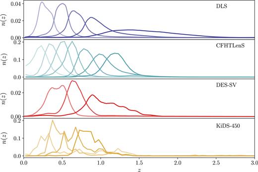
Estimation of the tomographic redshift distributions used in the four cosmic shear analyses. For DLS, CFHTLenS and DES-SV, stacked photometric redshift probability distribution functions (PDFs) were used; for KiDS-450, the redshift distribution of spectroscopic samples (weighted to match the source galaxies used for the cosmic shear analysis) were used. We see that DLS and CFHTLenS extend to higher redshift compared to DES-SV and KiDS-450.
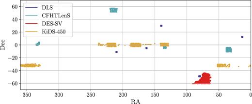
The location and footprints of the four surveys analysed in this paper. There is essentially no overlap between the footprints of the four surveys, except for a very small part of CFHTLenS and KiDS-450 at (RA, Dec) ≈ (130, -3) deg. We note that the projection in this plot does not reflect the relative area of the four surveys.
Characteristics of the four surveys and some of the modelling choices in each of the analyses.
| Parameters | DLS | CFHTLenS | DES-SV | KiDS-450 |
|---|---|---|---|---|
| Reference | Jee et al. (2016) | Joudaki et al. (2017a) | DES Collaboration (2016) | Hildebrandt et al. (2017) |
| Area (deg2) | 18 | 94 | 139 | 360 |
| Mean redshift | [0.45, 0.62, 0.75, | [0.35, 0.42, 0.50, 0.64 | [0.44, 0.67, 1.03] | [0.50, 0.49, 0.68, 0.85] |
| 1.04, 1.51] | 0.88, 1.06, 1.20] | |||
| σe (per component) | [0.25, 0.25, 0.25, | [0.28, 0.28, 0.28, 0.28, | [0.27, 0.28, 0.28] | [0.29, 0.28, 0.27, 0.28] |
| 0.25, 0.25] | 0.28, 0.28, 0.28] | |||
| |$n_{\rm eff}^{a}$| (arcmin−2) | [3.15, 3.58, 3.02, | [1.28,1.10,1.11,1.59, | [1.97, 2.03, 2.13] | [2.31,1.83,1.80,1.45] |
| 2.91, 3.75] | 2.74,1.75,0.87] | |||
| ξ+ θmin (arcmin) | 1.0 | 1.0 | 4.6/2.0b | 0.5 |
| ξ+ θmax (arcmin) | 90.0 | 60.0 | 60.0 | 72.0 |
| ξ− θmin (arcmin) | 1.0 | 8.0 | 56.5/24.5c | 4.2 |
| ξ− θmax (arcmin) | 90.0 | 120.0 | 300.0 | 300.0 |
| Data vector length | 240 | 280 | 36 | 130 |
| Covariance | 2048 simulations | 1988 simulations | 126 simulations | analytic |
| Cosmology inference | cosmopmc | cosmomc | cosmosis | cosmomc |
Notes.aWe adopt the definition used in Heymans et al. (2012), where |$n_{\rm eff} = A^{-1} (\Sigma _{i} w_{i})^{2} / \Sigma _{i} w_{i}^{2}$|. A is the area of the survey while |$w$|i is the weight for source galaxy i. The summation runs over all source galaxies.
bOnly for |$\xi _{+}^{23}$| and |$\xi _{+}^{33}$|, the small-scale cutoff is 2 arcmin.
cOnly for |$\xi _{-}^{11}$| and |$\xi _{-}^{12}$|, the small-scale cutoff is 60 arcmin.
2.1 DLS: the deep lens survey
The DLS (Wittman et al. 2000) consists of five ∼2 × 2 deg2 fields that add up to ∼18 deg2. Two fields were observed by the Kitt Peak Mayall 4 m telescope/Mosaic Prime-Focus Imager (Muller et al. 1998), and the other two by the Cerro Tololo Blanco 4 m telescope/Mosaic Prime-Focus Imager. The total DLS data set was taken over 140 nights of B, V, R, and |$z$| imaging. The approximate limiting magnitudes for each band (at 5σ) are 26, 26, 27, 26 in B, V, R and |$z$|, respectively. The average seeing is ∼0.9 arcsec in R.
The cosmic shear cosmology analysis from DLS was first presented in Jee et al. (2013), and later updated with Jee et al. (2016), which is the analysis we focus on in this paper. The shear measurement method is described in Jee et al. (2013), where an elliptical Gaussian galaxy model is used and image simulations (Jee & Tyson 2011) were employed for calibration of the shear estimate. The photometric redshift (or, photo-z) estimation uses the bpz code (Benítez 2000) and is validated against the PRIsm MUlti-object Survey (PRIMUS, Coil et al. 2011) in Jee et al. (2013).
DLS is the deepest survey with the smallest area of all the four data sets used in this work. As we do not have access to the shape catalogues for DLS, we start from the pre-measured two-point correlation functions provided by the collaboration.
2.2 CFHTLenS: the Canada–France–Hawaii Telescope Lensing Survey
The CFHTLenS data (Heymans et al. 2012; Erben et al. 2013) spans four distinct contiguous fields of approximately 63.8, 22.6, 44.2, and 23.3 deg2. Images are taken via the Canada–France–Hawaii 3.6m Telescope/MegaCam Imager in six filter bands: u*, g′, r′, i′, y′, |$z$|. The limiting magnitudes for each band (at 5σ in 2 arcsec aperture) are 25.24, 25.58, 24.88, 24.54, 24.71, 23.46 in the six bands, respectively, while the average seeing is 0.68 arcsec in i′, where the shapes are measured.
The cosmic shear cosmology analysis from CFHTLenS was presented first in Fu et al. (2008) and later updated in Heymans et al. (2013), Kilbinger et al. (2013), and then Joudaki et al. (2017a), which is the focus of this paper. The shear measurement was based on the lensfit package (Miller et al. 2007), which is a likelihood-based model-fitting approach that allows for joint-fitting over multiple observations of the same galaxy. A two-component (disc plus bulge) model is used to fit the galaxy shape and to extract the galaxy ellipticity. The method marginalizes over nuisance parameters such as galaxy position, size, brightness, and bulge fraction. Miller et al. (2013) describes the simulation-based calibrations that are applied to the shear catalogue. The photo-z estimation was based on the bpz code (Benítez 2000; Hildebrandt et al. 2012). The catalogues are publicly available.2 As seen in Fig. 1, the CFHTLenS analysis uses the largest number of tomographic bins.
In addition, in Joudaki et al. (2017a) extensive explorations of the impact of different intrinsic alignment (IA) models, baryonic feedback models, and photo-z uncertainties were performed. When considered independently, only the IA amplitude was found to be substantially favoured by the CFHTLenS data. However, with a 2σ negative amplitude, this could be a sign of either simplistic modelling or unaccounted systematics. The CFHTLenS analysis further considered joint accounts of the systematic uncertainties, where the ‘MIN’, ‘MID’, and ‘MAX’ cases included successively conservative treatments of the systematics modelling and scale cuts (along with a ‘fiducial’ case that included no systematics). Joudaki et al. (2017a) found that the S8 constraints were sensitive to the specific treatment of the systematic uncertainties, where the level of concordance with Planck ranged from decisive discordance (MIN) to substantial concordance (MAX). As a result, when quoting the nominal constraints from the collaboration, we show all three cases for CFHTLenS.
2.3 DES-SV: the Dark Energy Survey Science Verification Data
The DES-SV data set was taken before the official DES run began and was designed to cover a smaller area (∼250 deg2) to the full depth expected for DES. The area used in the cosmology analysis is a contiguous area of 139 deg2. Images were taken with the Dark Energy Camera (Flaugher et al. 2015) on the Cerro Tololo Blanco 4m telescope. Five filter bands: g, r, i, |$z$|, Y were used to a median depth of g ∼ 24.0, r ∼ 23.9, i ∼ 23.0, and |$z$| ∼ 22.3, respectively. The average seeing is 1.11 arcsec in r, 1.08 arcsec in i, and 1.03 arcsec in |$z$| – the DES-SV galaxy shapes used information from all three bands.
The cosmology analysis from weak lensing was presented in DES Collaboration (2016), while the details and testing of the measurements were recorded in Becker et al. (2016). Two independent shear catalogues were produced from the DES-SV data and have been extensively tested in Jarvis et al. (2016). In this work we use the catalogue produced by the shear measurement algorithm ngmix (Sheldon 2014), which is a fast Bayesian fitting algorithm that models galaxies as a mixture of Gaussian profiles. The Gaussian profiles are chosen to approximate an exponential disc. Several photo-z algorithms were tested in Becker et al. (2016) and Bonnett et al. (2016) including skynet (Bonnett 2015) and bpz (Benítez 2000). In DES Collaboration (2016), results from all shear and photo-z catalogues were presented and shown to be consistent. In this work we use only the ngmix catalogue and the skynet photo-z, as these were recommended by DES as the fiducial catalogues with the best performance. All catalogues are publicly available.3
The analysis pipeline used in DES Collaboration (2016) is based on comosis (Zuntz et al. 2015), which is the same cosmology inference framework we use in this paper, so we expect very good agreement between our analysis and DES Collaboration (2016).
2.4 KiDS-450: the 450 deg2 Kilo-Degree Survey
The KiDS-450 data set consists of five separate patches covering a total effective area of ∼360 deg2. Data were taken using the OmegaCAM CCD Mosaic camera mounted at the Cassegrain focus of the VLT Survey Telescope (VST). There are four SDSS-like filter bands, u, g, r, i, and the image depth is approximately 24.3, 25.1, 24.9, 23.8 in each band, respectively (5σ limit in 2 arcsec aperture). The median seeing is 0.66 arcsec in r, and no r-band images have seeing greater than 0.96 arcsec.
The cosmology analysis from cosmic shear using KiDS-450 data was presented in Hildebrandt et al. (2017). The cosmological inference pipeline was largely based on that used in CFHTLenS (Joudaki et al. 2017a), while several updates were made to the measurement pipeline. First, the shear calibration to the lensfit shear catalogue was based on more sophisticated image simulations (Fenech Conti et al. 2017). Secondly, a new approach for estimating photo-z and propagating photo-z uncertainties into cosmological inferences was implemented, which we briefly describe below.
The n(|$z$|) estimation in KiDS-450 is based on ideas presented in Lima et al. (2008) and implemented in Bonnett et al. (2016). This approach is referred to in Hildebrandt et al. (2017) as the ‘weighted direct calibration (DIR)’ method. The n(|$z$|) is taken directly from the redshift distribution of a spectroscopic sample with appropriate re-weighting in the colour-magnitude space to correct for the incompleteness and selection effects in both the shear catalogue and the spectroscopic sample. Since the n(|$z$|)’s are derived from a small number of spectroscopic galaxies, they appear more noisy than the other surveys in Fig. 1, where more traditional photo-z methods (stacked redshift probability distribution functions, or PDFs) are used.
3 PIPELINE
A directed acyclic graph (DAG) representing the modular pipeline developed for this analysis is shown in Fig. 3. The pipeline is implemented using the pegasus (Deelman et al. 2015) workflow management system. The individual components in the DAG are explained in more detail in Section 4, but we outline below the basic structure of the pipeline. Starting from the top, catalogues from each survey are fed into the first two branches of the pipeline which are run in parallel. The first branch (the left half of the DAG) starts with performing sample selection and tomographic binning by sorting catalogue data into Nt redshift bins and applying appropriate quality cuts, producing one intermediate catalogue file per bin. Next, Nc = Nt(Nt + 1)/2 jobs are launched in parallel to calculate the two-point shear correlation functions using the treecorr4 code. The output of all the parallel jobs is collected to form the data vector for the analysis. The second branch (the right half of the DAG) starts with estimating the full redshift distribution n(|$z$|) by summing the redshift PDFs for each individual galaxy.5 This approach of stacking the redshift PDFs for cosmological inference is not mathematically correct, but is consistent with the implementation of the four surveys under study. The n(|$z$|), together with other metadata from each survey (the effective number densities for each tomographic bin, the total shape noise, the survey area) are fed into the calculation of the analytic covariance corresponding to the data vector using the code cosmolike (Krause & Eifler 2017). A total of Nc(2Nc + 1) cosmolike jobs are launched to calculate each submatrix of the full covariance matrix in parallel. The results for all submatrices are then combined to form the full covariance.
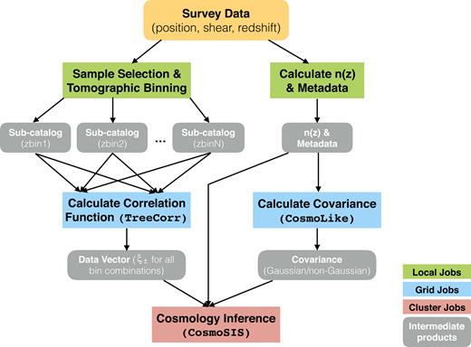
Flow chart of steps used in pipeline that goes from survey data to cosmology. The arrow pointing towards the left from the ‘n(|$z$|) & Metadata’ box bypasses the covariance calculation – it refers to the route taken when the survey-provided covariances are used in the inference.
Finally, the outputs from the two branches – the data vector and the covariance matrix – are fed into cosmosis (Zuntz et al. 2015) for inference of the cosmological model. The last step also involves choosing the appropriate theory models, priors, and scale cuts within cosmosis.
This pipeline is written in a modular and generic fashion that strings together the three main codes that are used: treecorr, cosmolike, and cosmosis, so that it is easy to substitute different input catalogues, covariances, and theory models. Building on this pipeline, it is easy to incorporate other cosmological probes, though that is beyond the scope of this paper. We note also that wlpipe serves as a test ground for experimenting on different pipeline architecture for future DESC cosmology analyses. For example, we have tested wlpipe using other workflow engines such as Parsl6 (Babuji Chard & Duede 2017). A similar pipeline was previously constructed for the recent DES Year 1 weak lensing and large-scale structure analyses (DES Collaboration 2018), the cosmic shear part (Troxel et al. 2018a) of which was made available to this project. The DES pipeline, however, did not employ any formal workflow management engine. The two pipelines have since been validated against one another to ensure they produce consistent results.
All plots of the cosmological constraints from cosmosis chains are plotted using the software package chainconsumer7 with setting kde = 1.5.
4 COMPARISON FRAMEWORK
The focus of this paper is to compare the cosmic shear analyses of the four precursor surveys in multiple aspects, both within the same data set and across the four data sets. We describe below the different elements that we consider in this work. We note that as our goal was to investigate and compare the various existing (published) data sets, there was no attempt of blinding throughout the analysis.
4.1 Two-point correlation functions
4.2 Covariance matrices
The covariance matrix is an essential element in the pipeline. The full covariance matrix receives contributions from two terms (Cooray & Hu 2001; Sato et al. 2009; Takada & Hu 2013): the Gaussian covariance and the non-Gaussian covariance. The non-Gaussian covariance includes the super-sample covariance (Takada & Hu 2013), which describes the uncertainty induced by large-scale density modes outside the survey window. In this work we use two sets of covariance matrices for each analysis: First, we use the covariance matrices used in the four papers (DES Collaboration 2016; Jee et al. 2016; Hildebrandt et al. 2017; Joudaki et al. 2017a), which were provided by the collaborations. Next, we use a theoretical Gaussian covariance matrix produced by the cosmolike (Krause & Eifler 2017) code. We note that the Gaussian covariance may not be sufficient, especially for DLS, given the smaller area and lower shape noise in this data set. For further details of the covariance calculation, see Krause et al. (2017). The cosmolike covariance calculation requires the following information from each survey:
n(|$z$|): estimate of redshift distribution for each tomographic bin (see Fig. 1)
neff: the effective number of source galaxies used in each bin as defined in Heymans et al. (2012) (see Table 1)
σe: standard deviation of the galaxy shape (or, shape noise) for the whole catalogue (see Table 1)
Asky: area of footprint (see Table 1).
We first use the survey-provided covariance to check whether we can reproduce the results from the papers. Next, we compare the cosmological constraints derived using the survey-provided and the theoretical Gaussian covariance. The four surveys have different approaches to estimate the covariance: for DLS, DES-SV, and CFHTLenS, the covariance was estimated via simulations (which are also different between the three cases). For KiDS-450, both simulation and analytic covariances were used and shown to be broadly consistent (though can cause a 1σ shift in the S8 constraints, see Hildebrandt et al. 2017). The final results were based on the analytic covariance.
4.3 Cosmological/Nuisance parameters
In all four survey analyses, of order 10 cosmological parameters and parameters modelling systematic effects are varied. The parameters each survey chooses to vary are slightly different and the corresponding priors are also different. In Table 2, we summarize the free cosmological/nuisance parameters and priors for the four analyses under the ΛCDM framework. We note that for CFHTLenS we have chosen to study the ‘fiducial’ setting in Joudaki et al. (2017a), which does not consider any systematic effects. In later analyses when we unify the analysis choices across surveys, the shear calibration bias, photo-z bias, and IA amplitude will be allowed to vary. We also note that in Table 2 there are two classes of parametrization of the free cosmological parameters. For DLS and DES-SV, [Ωm, Ωb, h, σ8, ns] was used, whereas for CFHTLenS and KiDS-450, [Ωch2, Ωbh2, h, ln (1010As), ns] was used. Here, Ωb is the baryon density today, h is the unitless Hubble constant (H0 = 100 h km−1 s−1 Mpc−1), σ8 is the amplitude of the (linear) power spectrum on the scale of 8 h−1Mpc, Ωc is the cold dark matter density today, As is the amplitude of the matter power spectrum, and ns is the spectral index. Since the priors on the varied parameters are taken to be flat, choosing Ωbh2 for example instead of Ωb translates to choosing a differently shaped prior on the Ωb − h parameter space. Furthermore, for CFHTLenS and KiDS-450, the h prior is an indirect one that depends on θMC, defined as 100 times the ratio of the sound horizon to the angular diameter distance, and is imposed at an intermediate stage. The effective prior on h is therefore not flat. As discussed in Hildebrandt et al. (2017) and Troxel et al. (2018b), however, this only has a small effect on the tails of the parameter constraints.
Free parameters in the cosmology inference used in Section 5.1, i.e. matching certain cases of the published results as closely as possible. The brackets indicate flat priors with [min, max] and the parentheses indicate Gaussian priors with (mean, standard deviation). We note that for CFHTLenS we choose to use the ‘fiducial’ setting in Joudaki et al. (2017a) as the Baseline, which does not consider any systematic effects. In later analyses when we unify the analysis choices across surveys, the shear calibration bias, photo-z bias, and IA amplitude will be allowed to vary.
| DLS | CFHTLenS | DES-SV | KiDS-450 | |
|---|---|---|---|---|
| Cosmology | Ωm: [0.01, 1.0] | Ωch2: [0.001, 0.99] | Ωm: [0.05, 0.9] | Ωch2: [0.01, 0.99] |
| Ωb: [0.03, 0.06] | Ωbh2: [0.013, 0.033] | Ωb: [0.02, 0.07] | Ωbh2: [0.019, 0.026] | |
| σ8: [0.1, 1.2] | ln (1010As): [2.3, 5.0] | σ8: [0.2, 1.6] | ln (1010As): [1.7, 5.0] | |
| h: [0.6, 0.8] | h: [0.61, 0.81]a | h: [0.3, 1] | h: [0.64, 0.82]a | |
| ns: [0.92, 1.02] | ns: [0.7, 1.3] | ns: [0.7, 1.3] | ns: [0.7, 1.3] | |
| Intrinsic alignment | AIA: 0.0 | AIA: 0.0 | AIA: [-5,5] | AIA: [−6,6] |
| Photo-z bias | b|$z$|: [−0.03, 0.03]b | 0 | b|$z$|, 1: (0, 0.05) | b|$z$|, 1: (0, 0.036) |
| b|$z$|, 2: (0, 0.05) | b|$z$|, 2: (0, 0.015) | |||
| b|$z$|, 3: (0, 0.05) | b|$z$|, 3: (0, 0.01) | |||
| b|$z$|, 4: (0, 0.006) | ||||
| Shear calibration bias | m: [−0.03, 0.03]b | 0 | m1: (0, 0.05) | m1: (0, 0.01) |
| m2: (0, 0.05) | m2: (0, 0.01) | |||
| m3: (0, 0.05) | m3: (0, 0.01) | |||
| m4: (0, 0.01) |
Notes.aPriors were placed in an intermediate stage.
bBins are assumed to be 100 per cent correlated.
The three classes of nuisance parameters considered here are defined as follows:
- Intrinsic alignment: Most current lensing surveys use the non-linear alignment model (NLA) proposed by Hirata & Seljak (2004), Bridle & King (2007), Joachimi et al. (2011). The model assumes that the IA power spectra PII and PGI scale with the non-linear power spectrum Pδ and can be redshift and luminosity-dependent:where(8)\begin{eqnarray*} P_{\rm II}(k,z) = F^{2} P_{\delta }(k,z); \,\, P_{\rm GI}(k,z) = F P_{\delta }(k,z), \end{eqnarray*}Here, AIA is a free parameter that dictates the amplitude of the effect, |$C_{1}=5\times 10^{-14}h^{-2}M_{\odot }^{-1}$|Mpc3 is a constant, ρcrit is the critical density at redshift zero, and D+(|$z$|) is the linear growth factor that is normalized to 1 today. The power laws η and β determine the redshift and luminosity evolution of the IA effect with |$z$|0 and L0 chosen as the anchoring redshift and luminosity. |$\bar{L}$| is the mean luminosity of the sample. In the four surveys considered in this work, DLS varied AIA, η, and β, the ‘MID’ case of CFHTLenS varied AIA, η, while the ‘MIN’ case of CFHTLenS, DES-SV, and KiDS-450 only varied AIA.11(9)\begin{eqnarray*} F(z, \bar{L}) = -A_{\rm IA}C_{1}\rho _{\rm crit} \frac{\Omega _{\rm m}}{D_{+}(z)} \left(\frac{1+z}{1+z_{0}}\right)^{\eta } \left(\frac{\bar{L}}{L_{0}} \right)^{\beta }. \end{eqnarray*}
- Photo-z uncertainty: The n(|$z$|) estimation can be uncertain and one should marginalize over this uncertainty. We parametrize this uncertainty following the approach used in DLS, CFHTLenS, and DES-SV (also see Huterer et al. 2006). That is, we assume the true redshift distribution n(|$z$|) has the same shape as the measured redshift distribution nobs(|$z$|), but has an uncertain shift in the mean of the distribution, b|$z$|,i, for each redshift bin i so thatThe approach used in KiDS-450 is slightly different, where the variation in the n(|$z$|) itself and the correlation between the errors is accounted for directly. This is done by running a large number (750 is used in Hildebrandt et al. 2017) of chains for each cosmological inference, where each chain uses a different bootstrap sample of the n(|$z$|), and combining all the chains at the very end. As the current wlpipe is not able to implement this operation, we calculate the standard deviation of the mean redshift for each of the 1000 bootstrap n(|$z$|)’s provided by the collaboration to be [0.036, 0.015, 0.010, 0.006] for each of the redshift bins, and use these values as the priors on the photo-z uncertainty the same way as the other surveys. We find that this approximation gives consistent results to the KiDS-450 approach. The one other subtle point is that in the DLS analysis, the photo-z biases are assumed to be 100 per cent correlated across redshift bins.(10)\begin{eqnarray*} n_{i}(z) = n_{{\rm obs}, i}(z-b_{z,i}). \end{eqnarray*}
- Shear calibration uncertainty: The shear measurements in each catalogue can be uncertain due to imperfect calibration (Mandelbaum et al. 2015). A common way of parametrizing this uncertainty is assuming the true shear γ scales linearly with the measured shear γobs by a factor (1 + mi) for each redshift bin i, plus an additive term ci (Heymans et al. 2006). That is(11)\begin{eqnarray*} \gamma _{\rm obs} = \gamma (1+m_{i}) + c_{i}. \end{eqnarray*}
As we will discuss in Section 5.1.4, the uncertainty in mi can either be incorporated at the parameter level or directly in the covariance matrix. We choose the former approach but show that the resulting cosmological constraints are identical (see Fig. B1 in Appendix B). The one other subtle point is that in the DLS analysis, the shear calibration uncertainties are assumed to be 100 per cent correlated across redshift bins. Finally, all surveys we analysed assume that any residual additive shear biases, ci, are negligible for the scales used.
In Section 5.4, we compare the cosmological constraints from the four data sets using the same priors on cosmological parameters and IA parameters. To see the effect of varying different combinations of the cosmological parameters discussed above, we run analyses for both the DES-SV priors and the KiDS-450 priors. For the photo-z and shear calibration parameters, however, we do not attempt to match between the surveys, as these are parameters that are characterized using the specific data sets. It would be incorrect to assume they have identical priors.
One final subtlety on the modelling side concerns the non-linear matter power spectrum. Amongst the surveys considered here, DLS uses the Smith et al. (2003) halofit power spectrum, CFHTLenS and KiDS-450 use the hmcode power spectrum, which is based on Mead et al. (2015), and DES-SV uses the Takahashi et al. (2012) halofit power spectrum. The difference in these power spectrum models can result in slightly shifted cosmological constraints, as discussed in Jee et al. (2016); Joudaki et al. (2017a,b); MacCrann et al. (2015). In this work we use the Takahashi et al. (2012) halofit power spectrum.
4.4 Scale cuts
In the four cosmic shear analyses, choices were made for which scales will be used for the cosmological inference. The choices were often based on considerations of systematic effects and model uncertainties. In general, the minimum scale is determined by model uncertainties such as baryonic physics and the accuracy of the non-linear power spectrum. The maximum scale cuts are usually related to survey-specific considerations such as the size of the footprint, additive shear bias, and super-sample covariance. For the four surveys considered, different choices of scale cuts were used and listed in Table 1. A few things to point out: For DLS, the same scale cuts were chosen for ξ+ and ξ−, though a discussion of how the scale cuts would change the cosmological constraints was presented in Jee et al. (2016). For CFHTLenS and KiDS-450, in addition to the motivations described above, scales with low signal-to-noise were also removed. Also, the use of smaller scales was justified since the effect of baryonic effects were modelled and marginalized over. For DES-SV, the scale cuts are redshift-dependent and the most conservative.
The physical scale cuts Rmin, ± chosen in our common analysis are Rmin, + =1.3 Mpc for ξ+ and Rmin, − =11.4 Mpc for ξ−. These choices are equal to the most conservative scale cuts amongst the four data sets and very similar to the DES-SV scale cuts. We note that we use Rmin, ± to translate the angular scale cuts between different redshift ranges. The reason for a larger Rmin, − is mainly reflecting the difference between the J0 and J4 Bessel functions in equation (1). We also note that for a more rigorous approach of using truly ‘linear scale’ cuts, see Section 3.5 of Joudaki et al. (2017a).
4.5 Cosmological constraints and comparisons metrics
In the next section, we will focus our comparison discussions surrounding four quantities:
- Signal-to-noise (S/N): This is simplyand it quantifies the statistical significance of the observables.(15)\begin{eqnarray*} S/N = \left[\sum _{i,j} d_i C^{-1}{}_{ij} \, d_j \right]^{0.5}, \end{eqnarray*}
Goodness of fit (χ2/ν, p.t.e.): For the best-fit data vector |$\hat{D}$|, we can calculate the χ2 per effective number of degree of freedom ν, and the corresponding probability-to-exceed (p.t.e.). It is important to evaluate the goodness of fit for each of the chains in parallel to check for consistency. One disadvantage for using the goodness of fit is that the determination of the degree of freedom in a high dimensional space is not straightforward. However, for this work the length of the data vector usually dominates over the number of model parameters.
- 1D distance in S8 (ΔS8): We calculate the ratio of the absolute difference between the mean parameter values in the two experiments and the uncertainty in the difference. For two experiments a and b, we thus haveΔS8 can roughly be interpreted as an n-σ difference in S8 for the two experiments. This metric inherently assumes Gaussianity in the S8 posterior and ignores possible tensions in other parameter projections. It can also overestimate the inferred disagreement when there are strong degeneracies in other parameter dimensions.(16)\begin{eqnarray*} \Delta S_{8} \equiv \frac{|S_{8}^{a}-S_{8}^{b}|}{\sqrt{\sigma (S_{8}^{a})^2+\sigma (S_{8}^{b})^2}}. \end{eqnarray*}
- Logarithmic Bayes Factor (BF): Based on Marshall, Rajguru & Slosar (2006), we consider the logarithmic ratio of the evidence for the two hypotheses: first that the two experiments are measuring the same cosmological parameters and second that they are measuring different cosmological parameters. That is, we calculateHere, the posteriors (including the priors) for each experiment Pa,b are integrated over all parameters |$\vec{p}$|. To properly interpret the BF values, one should evaluate it for cases where the two data sets share the same priors. As a result, we only calculate this at the end of the paper when all analysis choices are unified. We use the criteria BF > −1 to determine whether two surveys are consistent and can be combined. When BF < −1, the Jeffrey scale (Jeffreys 1961) suggests that there is effectively no evidence that the two data sets can be described by the same model.(17)\begin{eqnarray*} {\rm BF} = \log _{10} \left(\frac{\int d\Omega P_a(\vec{p}) P_b(\vec{p})}{[\int d\vec{p} P_a(\vec{p}) ][\int d \vec{p} P_b(\vec{p}) ]}\right). \end{eqnarray*}
We note, however, that the BF metric is sensitive to the priors on the constrained parameters, and is usually biased towards consistency (Raveri & Hu 2018).
5 RESULTS
In this section, we present the main results of this paper. In Section 5.1, we present results from the Baseline case: we set out to reproduce the results from the four published papers and discuss in detail the remaining differences between our reproduction and the published results, which we refer to as the Published Baseline. We also calculate several comparison metrics in order to understand the internal (external) consistency within (between) the four data sets. In Sections 5.2–5.4, we investigate individually the effect of changing the covariance estimation, the scale cuts, and the priors on cosmological parameters, and intrinsic alignment treatment. In Section 5.5, we unify the analysis choices and reexamine the comparison metrics. In Section 5.6, we discuss how the definition of S8 may affect the comparison between the surveys.
Throughout, we will also use the term Nominal Baseline to refer to the nominal analysis results that each collaboration uses as their most representative cosmological constraints, which for the case of CFHTLenS and KiDS-450 can be slightly different from the Published Baseline in terms of the treatment of systematic effects.
5.1 Baseline: reproducing literature results
The most basic test is the comparison of the literature results with the wlpipe’s measurements using the same catalogues under the same assumptions.
First, we examine the intermediate output of the measured ξ± functions. Fig. 4 shows ξ+(θ) and ξ−(θ) produced by wlpipe using the same binning and angular scales chosen by the collaborations, overlaid on top of results obtained by the collaborations for comparison. We find excellent agreement in all cases for the values of ξ±.12 Note that for DLS, CFHTLenS, and KiDS-450, the angular values for each data point assigned by wlpipe differ from the paper-provided data vectors. This, as we discussed in Section 4.1, is due to the fact that those paper-provided data vectors used the centre of each angular bin instead of the area-weighted centre. We show how this propagates into a bias in the cosmological constraints in Appendix A.
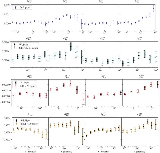
The 2-point function θξ±(θ) as measured by wlpipe from the catalogues provided by the collaborations compared with the results obtained by the collaborations themselves. For visualization purpose we only show the auto-correlation functions for the lowest and the highest redshift bins, and the colored data points are slightly displaced from the black points. From left to right in each panel is ξ+ for the lowest redshift bin, ξ+ for the highest redshift bin, ξ− for the lowest redshift bin, and ξ− for the highest redshift bin. From top to bottom are the four surveys: DLS, CFHTLens, DES-SV, and KiDS-450. Since the catalogues from DLS are not public, only the collaboration 2-point functions are shown in the top panel. We also note that the difference in the angular binning discussed in Section 5.1 is not shown in this plot, but explained more clearly in Appendix A.
Fig. 5 shows the constraints obtained from wlpipe for each experiment compared with those obtained by the collaborations themselves using the same binning, parameters, priors, and covariance matrices used to obtain the published results. In doing this we aim to reproduce the published results. However, Fig. 5 shows that there are differences between the published results and the wlpipe results, which we discuss in detail in the following subsections. The cosmosis configuration files and data files for these Baseline results are publicly available (Chang 2018).
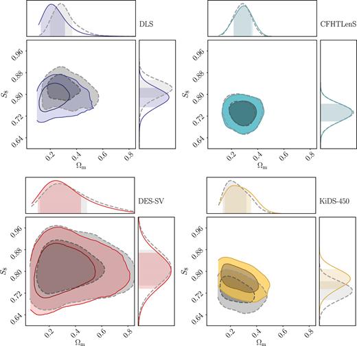
Results from reproducing published results with wlpipe. Here, we compare the marginalized constraints on Ωm and S8 ≡ σ8(Ωm/0.3)0.5 obtained from wlpipe (Baseline, solid colored contours) to those obtained by the collaborations (Published Baseline, dashed grey contours) for four different experiments. One can see clear shifts in the DLS and KiDS-450 contours. Section 5.1 describes all the factors that drive these discrepancies, and any accidental cancellations of effects for the other surveys.
5.1.1 DLS
From the upper left panel of Fig. 5, we see that the Published Baseline constraints from DLS are about 0.7σ higher in S8 and 0.5σ higher in Ωm than the Baseline constraints obtained via wlpipe. Differences in angular binning cannot be an issue here, since we are using the collaboration-computed ξ±. Two differences in the analysis explain the offset: First, the non-linear power spectrum used in the original DLS analysis of Jee et al. (2016) comes from an older version of halofit (Smith et al. 2003), while in cosmosis we use the non-linear power spectrum of Takahashi et al. (2012). As shown in MacCrann et al. (2015) and also discussed in section 6.3 of Jee et al. (2016), switching from the Smith et al. (2003) model to the Takahashi et al. (2012) model causes the inferred σ8 to be lowered by ∼0.02 at Ωm = 0.3. Secondly, as we have not implemented the particular IA model used in Jee et al. (2016) in wlpipe, we are assuming no IA in the wlpipe case. According to fig. 12 of Jee et al. (2016), this results in a ∼0.02 lower Ωm (with approximately the same S8). Accounting for these two factors brings the two contours to better agreement – where the wlpipe reproduction gives a slightly lower Ωm, but almost exactly the same S8 compared to the published results.
5.1.2 CFHTLenS
From the upper right panel of Fig. 5, we see that the published constraints from CFHTLenS are consistent with wlpipe in both the Ωm and S8 directions. We note that we have chosen to compare the ‘fiducial’ chain in Joudaki et al. (2017a), which does not include IA, baryons, photo-z uncertainties, or shear calibration uncertainties. Three factors need to be accounted for here: First, the angular values used in the paper-provided chains (the centre of the bin) are different from that in the wlpipe chain (equation 5). As we show in Appendix A, using the area-weighted angular values would shift the contours up by about 0.4σ. Secondly, whereas cosmosis uses the Takahashi et al. (2012) model in halofit, Joudaki et al. (2017a) used the slightly more accurate hmcode (Mead et al. 2016) for the non-linear power spectrum. As shown in fig. 10 of Joudaki et al. (2017a), the hmcode version used at that time moves the contour higher in S8 by about 0.4σ compared to halofit. These first two effects cancel, bringing the paper-provided chains and the wlpipe reproduction to perfect agreement. The final difference in our approaches is more subtle. As we noted in Section 4.3, CFHTLenS and KiDS-450 uses cosmomc, which does not sample h directly. Instead, it samples a wide flat prior in θMC (which is connected to h) and imposes the h priors after the fact. This means that the real h prior in the paper-provided chains is not exactly flat. This difference has been found to be small (Hildebrandt et al. 2017; Troxel et al. 2018b).
In Sections 5.1–5.4, we compare with the ‘fiducial’ case in Joudaki et al. (2017a) for simplicity. This assumes no systematic uncertainties, which according to fig. 12 of Joudaki et al. (2017a) and fig. 13, is close to the MID case in Joudaki et al. (2017a) (S8 is lower by 0.1σ). We do incorporate systematic uncertainties for CFHTLenS in Section 5.5 based on Kilbinger et al. (2017) and Choi et al. (2016).
5.1.3 DES-SV
We expect the wlpipe reproduction of the DES-SV Published Baseline results to be perfect up to noise in the sampling, since the analysis pipeline is almost identical in the two analyses (wlpipe uses slightly updated versions of treecorr, cosmolike, and cosmosis compared to that used in DES Collaboration 2016). As shown in the lower left panel of Fig. 5, this is indeed the case – the two contours agree very well.
5.1.4 KiDS-450
From the lower right panel of Fig. 5, we see that the Published Baseline constraints from KiDS-450 agree with the Baseline constraints from wlpipe in the Ωm direction and are about 0.9σ higher in the S8 direction. Several factors contribute to this discrepancy at different levels. First, the angular values used in the paper-provided chains (the centre of the bin) are different from those in the wlpipe chain (equation 5). Changing the bin values shifts the paper-provided chains up by about 0.4σ as shown in Fig. A1. Secondly, similar to CFHTLenS, the paper-provided chain uses hmcode for the non-linear power spectrum while wlpipe uses halofit. However, while Joudaki et al. (2017a) used the original version of hmcode (Mead 2015), a newer version of hmcode (Mead et al. 2016) was used in Hildebrandt et al. (2017). In this newer version, the fitting parameters were updated to allow for better fits when considering massive neutrino cosmologies, at the expense of slightly worse fits in standard ΛCDM. This newer version of hmcode agrees more strongly with halofit, and the resulting parameter constraints from KiDS-450 when using either prescription are almost identical (when excluding baryonic feedback). Thirdly, similar to CFHTLenS, θMC is varied in the analysis while h is a derived parameter. Fourthly, the covariance used in Hildebrandt et al. (2017) is designed to include the marginalization over multiplicative bias m, but was not implemented correctly (see also Fig. B1 and Troxel et al. 2018b). This moves the S8 constraints up by about 0.5σ. Finally, as described in Section 2.4, the photo-z uncertainties are incorporated differently in wlpipe compared to Hildebrandt et al. (2017). We have checked, however, that this does not generate any noticeable effect in the cosmological constraints.
In summary, we are able to reproduce the Hildebrandt et al. (2017) results in both Ωm and S8 when considering these factors. We note here that the fiducial analysis of Hildebrandt et al. (2017) includes modelling of the baryonic effects on small scales whereas we do not here. As a result we compare with their DIR chain, which as shown in fig. 8 of Hildebrandt et al. (2017) and Fig. 13, gives a S8 value 0.3σ lower than the Nominal Baseline case. Later when we unify the analysis choices, since we make much more conservative scale cuts, we do not expect the effect of baryons to be important.
5.1.5 Comparison of all four surveys
The right-hand panel of Fig. 6 shows the Baseline results from the four experiments using wlpipe in one plot, i.e. we overlay the coloured contours in Fig. 5 together. We note that here we have used the different analysis choices based on each of the collaborations, therefore the four contours cannot be compared on an equal footing. In this picture, we find good agreement between the four surveys in the Ωm − S8 plane, with CFHTLenS slightly lower than the other three surveys. DES-SV has the largest contour (weakest constraining power), whereas the other three surveys have contours of similar sizes. The degeneracy directions of the four surveys are somewhat different, as expected from the different redshift ranges they probe. For comparison, we also show in the left-hand panel of Fig. 6 the Published Baseline results from the corresponding survey-provided chains, or the four grey dashed contours in Fig. 5. The main difference from Fig. 5 is (1) the shifting of the KiDS-450 contours in the S8 direction, which comes from the change in the angular bin values and the covariance, as we discussed in Section 5.1.4 above, and (2) the DLS contours shifted to lower S8 due to the change in the non-linear power spectrum and the IA model, as we discussed in Section 5.1.1 above. This can also be seen more clearly comparing the Published Baseline and Baseline cases in Fig. 13.
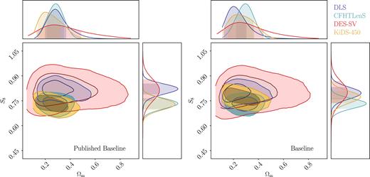
Here, we compare the constraints of the four surveys from the published results and the wlpipe reanalysis. We show the marginalized constraints on Ωm and S8 ≡ σ8(Ωm/0.3)0.5 from the paper-provided chains (the Published Baseline case, left-hand panel) and from wlpipe in the Baseline case. Note that compared to the Published Nominal results, here the KiDS-450 contours do not include baryonic effects, while the CFHTLenS contours do not include any systematic uncertainties.
We list the comparison metrics (as described in Section 4.5) for all the surveys as well as combinations of survey pairs for the chains in the Baseline case in Table 3. First, looking at the S/N, we notice that in the data configuration used in the individual surveys, the raw statistical power of the measurement is similar for DLS and CFHTLenS, while DES-SV is about half the S/N and KiDS-450 is in between. One interesting observation is that DLS achieves the high S/N even with a significantly smaller area – this highlights the power of having high-redshift data. A slightly worrying point is that the goodness of fits for DLS and CFHTLenS are quite low. For the pair-wise ΔS8, we find trends reflecting what is seen from the figures – all four surveys are broadly consistent with Table 3 showing some low-level discrepancies (1.5σ) in S8 between CFHTLenS and DLS.
Comparison metrics for all pairs of surveys in the Baseline analysis case: wlpipe chains that are designed to match the published analyses, or the Published Baseline case. For the S8 values, we list the mean and the 16 per cent and 84 per cent confidence intervals. We note that here we have used the different analysis choices based on each of the collaborations, so these metrics are not on equal footing. Later in Table 6 we show similar metrics that can be compared directly.
| (1) DLS | (2) CFHTLenS | (3) DES-SV | KiDS-450 | |
|---|---|---|---|---|
| S8 | |$0.795_{-0.032}^{+0.032}$| | |$0.731_{-0.028}^{+0.028}$| | |$0.802_{-0.058}^{+0.059}$| | |$0.770_{-0.034}^{+0.033}$| |
| S/N | 21.5 | 22.7 | 10.6 | 16.3 |
| χ2/ν | 334.8/235 | 417.6/275 | 26.9/30 | 122.4/124 |
| p.t.e. | 2.0 × 10⁻⁵ | 6.0 × 10⁻⁸ | 0.63 | 0.52 |
| ΔS8−(1) | – | 1.5 | 0.10 | 0.56 |
| ΔS8−(2) | – | – | 1.1 | 0.87 |
| ΔS8−(3) | – | – | – | 0.48 |
For the Published Baseline chains, we list the S8 constraints and ΔS8 values in Table 4. We do not list the goodness of fit here since they are not all available in the papers, and are not directly comparable with the values in Table 3. We just quote two numbers that are available: in Joudaki et al. (2017a), the reduced χ2 for the fiducial CFHTLenS analysis best-fit is 1.5, whereas in Hildebrandt et al. (2017), the reduced χ2 for the fiducial KiDS-450 analysis best-fit is 1.3. In Troxel et al. (2018b), it was shown that the reduced χ2 for the fiducial KiDS-450 improves to 1.0 when accounting for the survey geometry.
Comparison metrics for all pairs of surveys in the Published Baseline analysis case: constraints from the individual collaborations that we choose as baseline to reproduce. For the S8 values, we list the mean and the 16 per cent and 84 per cent confidence intervals. For CFHTLenS and KiDS-450, these are different from the Published Nominal analysis case: constraints from the individual collaborations that can be viewed as the representative results.
| (1) DLS | (2) CFHTLenS | (3) DES-SV | (4) KiDS-450 | |
|---|---|---|---|---|
| S8 | |$0.818_{-0.030}^{+0.030}$| | |$0.731_{-0.030}^{+0.030}$| | |$0.813_{-0.058}^{+0.059}$| | |$0.727_{-0.032}^{+0.033}$| |
| ΔS8−(1) | – | 2.1 | 0.076 | 2.1 |
| ΔS8−(2) | – | – | 1.2 | 0.087 |
| ΔS8−(3) | – | – | – | 1.3 |
5.2 Effect of the covariance matrix
Now we investigate the effect of the covariance matrix estimation. As discussed in Section 4.2, the four surveys have different approaches to covariance estimation. We eliminate these differences by generating a Gaussian analytical cosmolike covariance matrix for each survey.
Fig. 7 shows the changes in the contours in the four experiments when analytic covariance matrices are used in place of those provided by the collaborations. The corresponding comparison metrics are listed in Table 5. We notice shifts of the contours in the S8 constraints for some of the surveys. Overall, the Gaussian analytic covariance leads to slightly tighter constraints compared to covariance matrices estimated from simulations. This could be partially due to the fact that we have not accounted for the non-Gaussian piece of the analytic covariance.
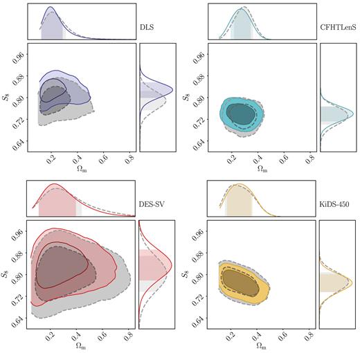
Effect of the covariance estimation – marginalized constraints on Ωm and S8 ≡ σ8(Ωm/0.3)0.5 obtained from wlpipe using the survey-provided covariance (grey dashed) for four different experiments and the cosmolike Gaussian analytic covariance (coloured solid). We can see a shift in the contours for DLS, CFHTLenS, and DES-SV.
S8 constraints, S/N, and goodness of fit when we change one analysis choice at a time in the analysis pipeline from the Baseline case (see Table 3). For the S8 values, we list the mean and the 16 per cent and 84 per cent confidence intervals. The sections of this table correspond to discussions in Sections 5.2–5.4.
| (1) DLS | (2) CFHTLenS | (3) DES-SV | (4) KiDS-450 | |
|---|---|---|---|---|
| Gaussian covariance matrix (Section 5.2) | ||||
| S8 | |$0.845_{-0.030}^{+0.030}$| | |$0.739_{-0.025}^{+0.024}$| | |$0.834_{-0.050}^{+0.052}$| | |$0.767_{-0.030}^{+0.030}$| |
| S/N | 26.0 | 22.2 | 12.7 | 20.4 |
| χ2/ν | 412.5/235 | 344.3/275 | 34.6/30 | 133.0/124 |
| p.t.e. | 7.0 × 10⁻¹² | 0.0028 | 0.26 | 0.27 |
| Conservative scale cuts (Section 5.3) | ||||
| S8 | |$0.928_{-0.050}^{+0.050}$| | |$0.731_{-0.050}^{+0.052}$| | |$0.799_{-0.069}^{+0.068}$| | |$0.754_{-0.055}^{+0.055}$| |
| S/N | 15.4 | 16.6 | 10.0 | 10.5 |
| χ2/ν | 112.1/89 | 228.3/132 | 28.4/25 | 62.8/56 |
| p.t.e. | 0.050 | 4.0 × 10⁻⁷ | 0.29 | 0.24 |
| DES-SV priors (Section 5.4) | ||||
| S8 | |$0.851_{-0.042}^{+0.042}$| | |$0.657_{-0.052}^{+0.052}$| | |$0.803_{-0.058}^{+0.059}$| | |$0.764_{-0.038}^{+0.038}$| |
| χ2/ν | 319.5/235 | 412.2/275 | 26.9/30 | 121.5/124 |
| p.t.e. | 2.0 × 10⁻⁴ | 1.6 × 10⁻⁷ | 0.63 | 0.55 |
| KiDS-450 priors (Section 5.4) | ||||
| S8 | |$0.818_{-0.033}^{+0.033}$| | |$0.677_{-0.039}^{+0.039}$| | |$0.807_{-0.059}^{+0.059}$| | |$0.771_{-0.033}^{+0.033}$| |
| χ2/ν | 323.6/235 | 412.5/275 | 27.0/30 | 122.2/124 |
| p.t.e. | 1.1 × 10⁻⁴ | 1.5 × 10⁻⁷ | 0.63 | 0.53 |
For DLS, we see a significant shift in the mean of the constraints towards higher S8 values; DES-SV and CFHTLenS also show some shifts in S8, but less significant. We note that, since the data vector is noisy, we do not expect the contours to agree exactly. However, we believe the shift for DLS is more than what is expected from statistical fluctuation. The DLS field is much smaller and contains a lower level of shape noise compared to the other surveys. In addition, one of the fields contains a galaxy cluster. These factors mean that the covariance is challenging to model and the simple Gaussian covariance used here may not be a good approximation for the data set. It is possible that neither the survey-provided covariance nor the Gaussian cosmolike covariance from wlpipe captures these complications. We also note that for the three cases where simulation covariance is used, DES-SV has the smallest Hartlap factor (HDLS = 0.88, HCFHTLenS = 0.86, HDES-SV = 0.7). This means that the inverse of the simulation covariance in DES-SV is expected to be noisier (but unbiased) compared to the other two simulation covariances (Dodelson & Schneider 2013).
Finally, it is also worth noting that since the survey-provided covariance from KiDS-450 is also an analytic covariance matrix, the agreement between the dashed and the solid contours in the bottom right of Fig. 7 is a good check on the analytic calculation for the covariance. We have checked that the slightly smaller contours from wlpipe is partially reflecting the difference between the Gaussian and non-Gaussian covariance.
5.3 Effect of scale cuts
In this section, we investigate the effect of scale cuts. Following Section 4.4, we choose to match all scale cuts to the most conservative scale cuts in the four data sets (Rmin, + >1.3 Mpc and Rmin, − > 11.4 Mpc, see equation 12). The results are shown in Fig. 8, with the corresponding metrics listed in Table 5. The exact cuts used in each bin are tabulated in Appendix C, Table C1. In all these tests, everything else in the analysis stays the same as the Baseline case in Section 5.1.
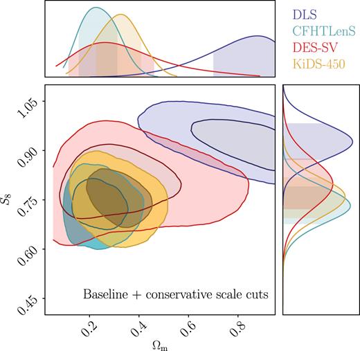
Effect of scale cuts compared to Baseline (right-hand panel of Fig. 6) – we show the marginalized constraints for Ωm and S8 ≡ σ8(Ωm/0.3)0.5 when small-scale data are removed from the fit (requiring Rmin, + > 1.3 Mpc and Rmin, - > 11.4 Mpc). DLS shifts to large Ωm and S8 values, while the other surveys show enlarged contours compared to Baseline. We note that the four contours should not be compared directly here, as the analysis choices are not unified.
In Fig. 8, the first thing that draws the eye is the DLS contours, which shift to very large Ωm values, as well as a higher S8. All the other surveys appear consistent with the original case in Fig. 6, but with looser constraints due to the fact that we have removed information.
We note that the goodness of fit for DLS improved significantly when applying the conservative scale cuts compared to the Baseline case. After a more careful look at the DLS measurements, it appears that the small-scale data points for ξ− is the source of the contour shift – those data points prefer a lower amplitude compared to the rest of the data points. Therefore, when applying the conservative scale cuts, the model amplitude increases (so does S8), and the goodness of fit improves. This could also be a hint that the small-scale covariance is underestimated, as already discussed in Section 5.2, that the characteristics of the DLS data makes it difficult to model the covariance. We note that some of these issues were discussed in Jee et al. (2013) and Jee et al. (2016), and a similar trend in S8 was seen in fig. 13 of Jee et al. (2016). Here, we caution that since the DLS contours are far from Ωm = 0.3 and clipped by the priors (Ωm < 1), the S8 values quoted are not very meaningful.
5.4 Impact of cosmological priors and IA treatment
Next, we consider the impact of different cosmological priors and IA treatments. To address this, we impose identical priors on all surveys, first using those from DES-SV and then from KiDS-450 (see Table 2) since they roughly represent the two approaches of handling the parameters: DES-SV has priors that are relatively conservative, and in the parametrization of [Ωm, Ωb, h, σ8, ns], whereas KiDS-450 has more restrictive priors and uses the parametrization [Ωch2, Ωbh2, h, ln (1010As), ns]. We moreover allow for intrinsic alignments in the case of CFHTLenS and DLS. For all surveys, we consider either the IA amplitude prior −5 < AIA < 5 used by DES-SV or the prior −6 < AIA < 6 used by KiDS-450. Note that aside from these changes to the cosmological priors and IA treatments, we keep all other analysis choices the same as in the Baseline case of Section 5.1.
The two panels of Fig. 9 show the effect of unifying the cosmological priors and IA treatments from that chosen as Baseline, with the corresponding metrics listed in Table 5. Looking at CFHTLenS, DES-SV, and KiDS-450, it is apparent that the constraints in the Ωm direction are largely dominated by cosmological priors. Specifically, the prior on h, which is wider for DES-SV compared to KiDS-450, leads to large changes in the Ωm posterior. The constraints on S8, on the other hand, are relatively robust to cosmological priors, consistent with previous findings (Kilbinger et al. 2013; Joudaki et al. 2017a). This again is showing that cosmic shear measurements for these four data sets are mainly constraining only the amplitude of the power spectrum and not the detailed shape of it. The uncertainty on S8 decreases for CFHTLenS when moving to tighter cosmological priors, however, this is largely due to the fact that the S8 definition here is not optimal for the CFHTLenS data set. We will discuss this point in Section 5.6.
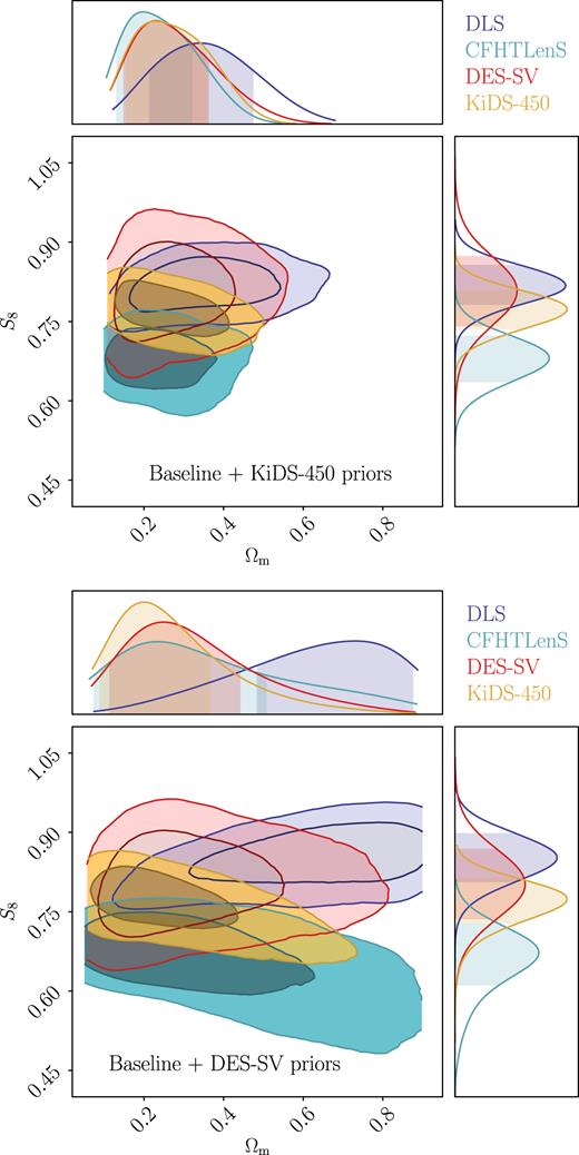
Impact of cosmological priors and IA treatments compared to Baseline (right-hand panel of Fig. 6) – we show the marginalized constraints for Ωm and S8 ≡ σ8(Ωm/0.3)0.5 when unifying the priors on the cosmological and IA parameters. We first unify to the KiDS-450 priors (top), then to the DES-SV priors (bottom). The constraints in the Ωm direction is heavily affected by the priors, while in the S8 direction, there is a larger effect for surveys with a strong degeneracy in the Ωm − S8 plane. We note that the four contours should not be compared directly here, as the analysis choices are not unified.
A few other effects of the cosmological priors and IA treatment are visible in Fig. 9. First, for DLS, when imposing the DES-SV priors, Ωm moves to high values while S8 remains roughly the same. When imposing KiDS-450 priors, the Ωm constraints appear similar to the Baseline case. This behaviour, together with what is shown in Section 5.3, suggests that the DLS constraints on Ωm are sensitive to the scales used and the priors. For CFHTLenS, the S8 constraints move to lower values using both DES-SV and KiDS-450 priors. This comes from the fact that compared to the Baseline case, here there is additional freedom in the IA amplitude. We examine the IA amplitude when using the KiDS-450 priors, as shown in Fig. 10, and find that the CFHTLenS favours a negative IA amplitude at the 2σ level. This, based on previous work in measurements of IA, suggests that we may be fitting to some systematic effects that appear to behave like IA (Choi et al. 2016; Kilbinger et al. 2017; van Uitert et al. 2018). This is consistent with figs 8 and 9 of Joudaki et al. (2017a), where they show that this negative IA shifts the S8 constraints to lower values. There is also a similar (but less severe) trend in the DLS data.
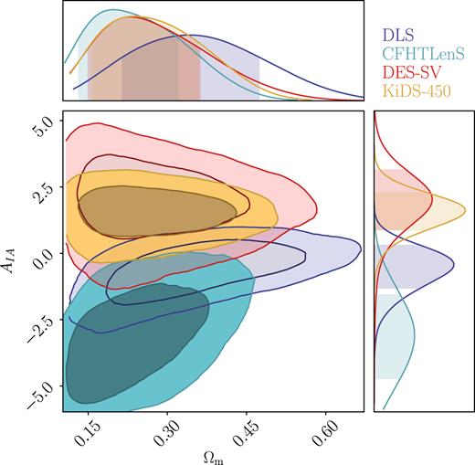
Constraints on IA amplitude – we show the marginalized constraints for Ωm and AIA when unifying the priors to the KiDS-450 priors (keeping all other analysis choices as in the Baseline case). We find a degeneracy between AIA and Ωm for DLS and CFHTLenS. We also find that both these surveys prefer negative IA amplitudes in this set-up.
5.5 Common covariances, angular scale cuts, cosmological priors, and IA treatments
After investigating the individual effects in Sections 5.2–5.4, we now combine all of them and perform a uniform analysis on all four surveys. We study two cases, both using cosmolike Gaussian covariances, conservative scale cuts, the same IA treatments, and we use two sets of priors:
KiDS-450 priors and
DES-SV priors.
As discussed in Section 5.1.2, in this subsection we incorporate the photo-z and shear calibration bias uncertainties for CFHTLenS. As summarized in section 4.3 of Kilbinger et al. (2017), a number of improvements to CFHTLenS have been identified since the public release of the catalogues in 2013. Of importance to this study is the analysis by Choi et al. (2016), who showed that significant biases existed in the reported photo-z distributions, the result from Kuijken et al. (2015) that the CFHTLenS shear calibration corrections were in general underestimated and the finding by Fenech Conti et al. (2017) that the previously unexplored area of galaxy selection bias results in a few per cent overestimation of the shear calibration correction. The conclusion of all these works was that any future analyses of CFHTLenS should include conservative systematic error terms to account for these effects. In this section, we therefore marginalize over an uncertainty in the mean redshift of each bin with zero-mean top-hat prior of full-width 0.2, and an uncertainty in the shear calibration correction zero-mean top-hat prior of full-width 0.1.
In Fig. 11 we show the comparison between the Published Nominal contours and case (i) listed above. The Published Nominal contours present the view one would have on the four cosmic shear surveys after reading the individual papers (DES Collaboration 2016; Jee et al. 2016; Hildebrandt et al. 2017; Joudaki et al. 2017a), while the Matched contours present what the cosmological constraints are when analysed through a unified analysis framework. One can also compare with Fig. 6 to understand the nature of the different changes in the contours. The contours for (ii) are shown in Fig. 12. We choose to focus on (i) here as it is not as affected by the S8 definition (see Section 5.6) as (ii). The four surveys in the right-hand panel of Fig. 11 can now be compared on equal footing. The comparison metrics are shown in Table 6.
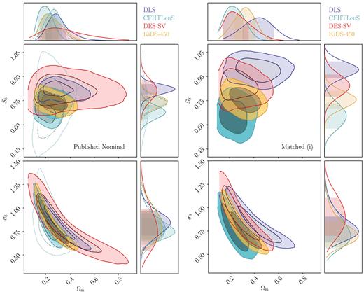
Final comparison of the cosmological constraints from the four surveys according to the literature (Published Nominal, left) and according to our unified analysis framework (right, Matched) – we show the marginalized constraints for Ωm, S8 ≡ σ8(Ωm/0.3)0.5 and σ8 for the four cosmic shear surveys. In the right-hand panel, we use Gaussian analytic covariances, conservative scale cuts, and the KiDS-450 priors. We note that for the CFHTLenS Published Nominal constraints, we show all three settings MIN (solid), MID (dashed), and MAX (dotted) in Joudaki et al. (2017a).

Same as the upper right panel of Fig. 11, but now using DES-SV priors.
Comparison metrics corresponding to the right-hand panel of Fig. 11. That is, all analysis choices matched: Gaussian cosmolike covariance matrix, conservative scale cuts, same IA treatments, and KiDS-450 cosmological priors. For the S8 values, we list the mean and the 16 per cent and 84 per cent confidence intervals.
| (1) DLS | (2) CFHTLenS | (3) DES-SV | (4) KiDS-450 | |
|---|---|---|---|---|
| S8 | |$0.942_{-0.045}^{+0.046}$| | |$0.657_{-0.070}^{+0.071}$| | |$0.844_{-0.061}^{+0.062}$| | |$0.755_{-0.049}^{+0.048}$| |
| S/N | 17.4 | 15.1 | 11.6 | 12.1 |
| χ2/ν | 137.8/89 | 176.3/132 | 32.7/26 | 71.5/56 |
| p.t.e. | 7.0 × 10⁻⁴ | 0.0060 | 0.17 | 0.079 |
| ΔS8−(1) | – | 3.4 | 1.3 | 2.9 |
| ΔS8−(2) | – | – | 2.0 | 1.1 |
| ΔS8−(3) | – | – | – | 1.2 |
| BF-(1) | – | −1.1 | 1.6 | −0.50 |
| BF-(2) | – | – | 0.70 | 1.3 |
| BF-(3) | – | – | – | 1.1 |
In general, we observe the same effects seen individually in Sections 5.2–5.4. But when put together, the discrepancies between the different surveys coming from the different effects accumulate and become larger. Looking at Fig. 11 and the ΔS8 statistics in Table 6, we find that essentially none of the surveys have S8 constraints that agree within 1σ and the extreme cases differ more than 3σ. If we look at the change in the S8 constraints for the individual surveys from the left-hand panel to the right-hand panel, it is clear that the main effect is that DLS moves to larger S8. CFHTLenS is consistent with the MIN and MAX case but not the MID case, which is expected given that the choice of IA models we use is the same as the MIN case, and that the MAX case has little constraining power. DES-SV and KiDS-450 stay roughly the same.
Next, we turn to the other statistics in Table 6. We note that the signal-to-noise for the four data sets change slightly, but the relative power stays roughly the same, with DLS being the highest and DES-SV being the lowest. We note that the goodness of fit for DLS and CFHTLenS improved from the Baseline case but is still quite low. The largest ΔS8 is about 3.4σ between DLS and CFHTLenS, which is also apparent from Fig. 11. Next, we look at the BF statistic (equation 17) between pairs of surveys. Here, when evaluating the numerator in equation (17) for BF, we only require the cosmological parameters to be shared amongst the two experiments being compared and keep the IA amplitude, shear calibration parameter, and photo-z uncertainty separate. We find that the message from the BF statistics is similar to that captured by the ΔS8 metric in this case, though the message of consistency/inconsistency is somewhat weaker – the only BF value that fails the requirement of combining is DLS and CFHTLenS.
We now combine the two surveys, DES-SV and KiDS-450, under this matched setting. These two data sets are consistent under the same model assumption according the BF metric, and have reasonable goodness-of-fit values. The combined constraint of DES-SV and KiDS-450 is |$S_{8}=0.790^{+0.042}_{-0.041}$|. Compared to the cosmic shear results from the first year DES data (Troxel et al. 2018a), |$S_8=0.789^{+0.024}_{-0.026}$|, we find excellent agreement. Compared to the state-of-the-art CMB constraints (Planck Collaboration VI 2018), |$S_{8}=0.832_{-0.013}^{+0.013}$|, we find reasonably consistent results with roughly 1σ lower S8. These results are in good agreement with that found in Troxel et al. (2018b).
5.6 A side note on the S8 definition
As discussed briefly in Section 4.5, S8 is defined as σ8(Ωm/0.3)α, where α is designed to remove the degeneracy between σ8 and Ωm. That is, if α is chosen optimally, it characterizes the direction orthogonal to the Ωm − σ8 contours. For data sets of different redshift distribution, the optimal α is different.
Throughout our analysis, we have fixed α to be 0.5, which may not be optimal for all data sets. This implies that for data sets where α is further from 0.5, the projected uncertainties on S8 = σ8(Ωm/0.3)0.5 are going to be slightly larger than if the optimal α were used, and that when comparing the different surveys they will tend towards being consistent. This can be seen clearly in Fig. 12, where the contours for CFHTLenS and KiDS-450 are tilted leading to larger uncertainties in the S8 direction. The effect is much reduced when a tighter prior is imposed as in the right-hand panels of Fig. 11. Roughly, we find that with the DES-SV priors (corresponding to Fig. 12), the optimal α values are 0.56 (DLS), 0.71 (CFHTLenS), 0.51 (DES-SV), and 0.67 (KiDS-450). With the KiDS-450 priors (corresponding to the right-hand panels of Fig. 11), the optimal α values are 0.52 (DLS), 0.52 (CFHTLenS), 0.52 (DES-SV), and 0.58 (KiDS-450). That is, we expect the discrepancies between the surveys in the single parameter that quantifies the amplitude to be sensitive to the priors and likely larger if an optimal α is used. On the other hand, the BF metric is insensitive to the choice of α so is a more robust measure of consistency.
6 SUMMARY AND DISCUSSION
In this paper, we use a generic cosmic shear pipeline, wlpipe, that takes in galaxy shear catalogues, calculates the two-point shear-shear correlation function via the software package treecorr and the associated covariance matrix via the software package cosmolike, and finally carries out cosmological parameter inference via the software package cosmosis. The wlpipe framework is constructed using the pegasus workflow engine, which takes care of data and code transfer between different computing resources seamlessly. This pipeline also serves as a prototype pipeline for future analysis pipelines in DESC.
We apply this pipeline to four existing cosmic shear surveys: DLS, CFHTLenS, DES-SV, and KiDS-450. The goal is to first reproduce the literature results, investigate the effect of different analysis choices adopted in each of the surveys, and finally unifying these different analysis choices in order to perform an apples-to-apples comparison of the survey results. In Fig. 13, we summarize the constraints on S8 ≡ σ8(Ωm/0.3)0.5 from all the cases studied in this work. We summarize our main findings below:
We are able to reproduce a specific set of the published results from the four collaborations when following the same analysis choices to well within the uncertainties. In this Baseline case, the four surveys appear to be broadly consistent in terms of their constraints on S8 ≡ σ8(Ωm/0.3)0.5: |$0.795_{-0.032}^{+0.032}$| (DLS), |$0.731_{-0.028}^{+0.028}$| (CFHTLenS), |$0.802_{-0.058}^{+0.059}$| (DES-SV), and |$0.770_{-0.034}^{+0.033}$| (KiDS-450). However, we note that not all the model fits are good descriptions of the data – for DLS and CFHTLenS, the p-values for the fits are low, while for KiDS-450, the p-value is acceptable, but only after incorporating recent improvements for the covariance.
In reproducing the published results, we investigate several issues in the published results: the angular bin values used in the data vector, the incorporation of nuisance parameters in the covariance, and the non-linear power spectrum model and others. We find these details can shift the cosmological constraints by ∼0.5σ. Most of these issues are known, but analysing all four experiments systematically in this work gives a big picture view of how the four analyses agree and differ.
Effect of the covariance matrix: constraints based on simulation-based covariances can be shifted from analytic covariances due to noise. In addition, the DLS covariance may not be well approximated by a Gaussian covariance due to the complexity of the data, the small area and the low shape noise.
Effect of scale cuts: sensitivity of the cosmological constraints to scale cuts could indicate internal inconsistency of data sets or further issues with the covariance. It could also point to potential failures in the models at small scales (e.g. IA, non-linear matter power spectrum, baryonic physics).
Effect of priors: for parameters that are not constrained (e.g. Ωm), the priors have an effect on the constraints, but for parameters that are constrained (e.g. S8), the effect of priors is smaller, but not negligible. A wide prior on the IA amplitude can absorb other sources of systematic issues, which could explain the slightly negative IA amplitude constrained by CFHTLenS.
When unifying all analysis choices discussed above, the four surveys give the following constraints: we find S8 ≡ σ8(Ωm/0.3)0.5 to be |$0.942_{-0.045}^{+0.046}$| (DLS), |$0.657_{-0.070}^{+0.071}$| (CFHTLenS), |$0.844_{-0.061}^{+0.062}$| (DES-SV), and |$0.755_{-0.049}^{+0.048}$| (KiDS-450). Specifically, DLS moves to higher S8 while CFHTLenS moves to lower S8 compared to the Baseline. The change in the DLS constraints is primarily due to the scale cuts and covariance, while the change in CFHTLenS is due to the change in the IA treatment, and could be an indication of residual issues in the photo-z estimation. The goodness-of-fit values for DLS and CFHTLenS improved but is still low.
We calculate the ΔS8 statistics and the Bayesian evidence ratio (BF) between each of the two surveys (when analysis choices are unified). The S8 constraints from the two most discrepant cases (DLS and CFHTLenS) differ by 3.4σ. The S8 constraints for DES-SV and KiDS-450 in the final matched analysis appear consistent with the Baseline analysis as well as with each other. They also seem to be robust to the various analysis choices tested. Together with the more reasonable goodness-of-fit values and IA constraints, this is an encouraging indication for the field given that DES-SV and KiDS-450 are the most recent work amongst the four surveys.
Based on all the above information, we decide to combine the DES-SV and KiDS-450 data sets (based on the goodness of fit, IA constraints, and consistency). The combined constraint is |$S_{8}=0.790^{+0.042}_{-0.041}$|, which is in agreement with both the cosmic shear constraints from the first year of DES data in Troxel et al. (2018a), and the CMB constraints from Planck Collaboration VI (2018).

Summary of S8 = σ8(Ωm/0.3)0.5 constraints from the four cosmic shear surveys studied in this work. Each bar shows the 16 per cent and 84 per cent confidence interval of the S8 constraints. The plot is divided by dashed horizontal lines into four sections. The first section shows chains provided by the respective collaborations. The second section shows constraints derived from wlpipe, but are not fully matched in all analysis steps, ergo not directly comparable. The third section shows constraints derived from wlpipe and have analysis steps matched, so can be compared directly. The last section shows the constraints from combining the two consistent surveys DES-SV and KiDS-450, the Planck satellite (Planck Collaboration VI 2018) and DES Y1 cosmic shear (Troxel et al. 2018a). The naming conventions are explained in the table below the figure. We note that for the CFHTLenS Published Nominal constraints, we show all three settings MIN (top), MID (middle) and MAX (bottom) in Joudaki et al. (2017a).
Cosmic shear measurements hold great promise in terms of the constraining power in cosmology. In order to fully exploit this power in upcoming and future cosmic shear surveys (DES, KiDS, HSC, Euclid13, LSST, Wide Field Infrared Survey Telescope14), it is important to learn from the experiences accumulated over the past years in the community across the different collaborations and data sets. We have demonstrated that a number of analysis choices can result in significant changes in the cosmological constraints and should therefore be treated with care for the future analyses.
ACKNOWLEDGEMENTS
We thank Hendrik Hildebrandt and Martin Kilbinger for helping with the KiDS-450 reanalysis. We thank Sebastian Bocquet, Francois Lanusse, and Javier Sanchez for help in the early stages of this project. We thank Weikang Lin and Mustapha Ishak for useful discussions regarding metrics for consistency. We thank Karan Vahi and Mats Rynge for support in using the Pegasus software. This paper has undergone internal review in the LSST Dark Energy Science Collaboration, with Bhuvnesh Jain, Niall MacCrann, and Marco Raveri as internal reviewers.
CC was supported in part by the Kavli Institute for Cosmological Physics at the University of Chicago through grant NSF PHY-1125897 and an endowment from Kavli Foundation and its founder Fred Kavli. CH acknowledges support from the European Research Council under grant number 647112. Support for MS was provided by the University of California Riverside Office of Research and Economic Development through the FIELDS NASA-MIRO programme. A portion of this research was carried out at the Jet Propulsion Laboratory, California Institute of Technology, under a contract with the National Aeronautics and Space Administration. MJJ acknowledges support for the current research from the National Research Foundation of Korea under the programme 2017R1A2B2004644 and 2017R1A4A1015178. RM is supported by the Department of Energy Cosmic Frontier programme, grant DE-SC0010118. SJ acknowledges support from the Beecroft Trust and ERC 693024. AIM is advised by David W. Hogg and was supported by National Science Foundation grant AST-1517237. Part of this work performed under the auspices of the U.S. Department of Energy by Lawrence Livermore National Laboratory under Contract DE-AC52- 07NA27344. This work was performed at the Aspen Center for Physics, which is supported by National Science Foundation grant PHY-1607611.
The DESC acknowledges ongoing support from the Institut National de Physique Nucléaire et de Physique des Particules in France; the Science & Technology Facilities Council in the United Kingdom; and the Department of Energy, the National Science Foundation, and the LSST Corporation in the United States. DESC uses resources of the IN2P3 Computing Center (CC-IN2P3–Lyon/Villeurbanne – France) funded by the Centre National de la Recherche Scientifique; the National Energy Research Scientific Computing Center, a DOE Office of Science User Facility supported by the Office of Science of the U.S. Department of Energy under Contract No. DE-AC02-05CH11231; STFC DiRAC HPC Facilities, funded by UK BIS National E-infrastructure capital grants; and the UK particle physics grid, supported by the GridPP Collaboration. This work was performed in part under DOE Contract DE-AC02-76SF00515.
Below we acknowledge the data sources:
CFHTLenS: This work is based on observations obtained with MegaPrime/MegaCam, a joint project of CFHT and CEA/IRFU, at the Canada–France–Hawaii Telescope (CFHT), which is operated by the National Research Council (NRC) of Canada, the Institut National des Sciences de l’Univers of the Centre National de la Recherche Scientifique (CNRS) of France, and the University of Hawaii. This research used the facilities of the Canadian Astronomy Data Centre operated by the National Research Council of Canada with the support of the Canadian Space Agency. CFHTLenS data processing was made possible thanks to significant computing support from the NSERC Research Tools and Instruments grant programme.
DES-SV: This project used public archival data from the Dark Energy Survey (DES). Funding for the DES Projects has been provided by the U.S. Department of Energy, the U.S. National Science Foundation, the Ministry of Science and Education of Spain, the Science and Technology Facilities Council of the United Kingdom, the Higher Education Funding Council for England, the National Center for Supercomputing Applications at the University of Illinois at Urbana-Champaign, the Kavli Institute of Cosmological Physics at the University of Chicago, the Center for Cosmology and Astro-Particle Physics at the Ohio State University, the Mitchell Institute for Fundamental Physics and Astronomy at Texas A&M University, Financiadora de Estudos e Projetos, Fundação Carlos Chagas Filho de Amparo à Pesquisa do Estado do Rio de Janeiro, Conselho Nacional de Desenvolvimento Científico e Tecnológico and the Ministério da Ciência, Tecnologia e Inovação, the Deutsche Forschungsgemeinschaft, and the Collaborating Institutions in the Dark Energy Survey. The Collaborating Institutions are Argonne National Laboratory, the University of California at Santa Cruz, the University of Cambridge, Centro de Investigaciones Energéticas, Medioambientales y Tecnológicas-Madrid, the University of Chicago, University College London, the DES-Brazil Consortium, the University of Edinburgh, the Eidgenössische Technische Hochschule (ETH) Zürich, Fermi National Accelerator Laboratory, the University of Illinois at Urbana-Champaign, the Institut de Ciències de l’Espai (IEEC/CSIC), the Institut de Física d’Altes Energies, Lawrence Berkeley National Laboratory, the Ludwig-Maximilians Universität München and the associated Excellence Cluster Universe, the University of Michigan, the National Optical Astronomy Observatory, the University of Nottingham, The Ohio State University, the OzDES Membership Consortium, the University of Pennsylvania, the University of Portsmouth, SLAC National Accelerator Laboratory, Stanford University, the University of Sussex, and Texas A&M University. Based in part on observations at Cerro Tololo Inter-American Observatory, National Optical Astronomy Observatory, which is operated by the Association of Universities for Research in Astronomy (AURA) under a cooperative agreement with the National Science Foundation.
KiDS-450: This work is based on data products from observations made with ESO Telescopes at the La Silla Paranal Observatory under programme IDs 177.A-3016, 177.A-3017, and 177.A-3018. We use cosmic shear measurements from the Kilo-Degree Survey (Kuijken et al. 2015; Fenech Conti et al. 2017; Hildebrandt et al. 2017), hereafter referred to as KiDS. The KiDS data are processed by THELI (Erben et al. 2013) and Astro-WISE (Begeman et al. 2013, de Jong et al. 2015). Shears are measured using lensfit (Miller et al. 2013), and photometric redshifts are obtained from PSF-matched photometry and calibrated using external overlapping spectroscopic surveys (see Hildebrandt et al. 2017).
The contributions from the primary authors are listed below. CC led the main analysis and writing of this paper. MW wrote the main software package wlpipe which integrates the python scripts using the Pegasus workflow engine. SD helped with the pipeline development, covariance assessment, comparison metrics, pipeline testing, and editing.
Footnotes
For a non-flat universe, one would replace χ by fK(χ) in the following equations, where K is the universe’s curvature, fK(χ) = K−1/2sin (K1/2χ) for K > 0 and fK(χ) = (− K)−1/2sinh ((− K)1/2χ) for K < 0.
We note that in the later analyses for the individual surveys, some of them do not provide redshift PDFs per galaxy. Instead, they provide the full n(|$z$|) for each redshift bin. In those cases (DLS and KiDS) we directly use the survey-provided n(|$z$|).
The shear response should also be included in the weights, but since the shear response is approximately homogeneous across the survey, we do not incorporate it into this calculation.
There is a small discrepancy between the published results and the wlpipe measurements for KiDS-450 due to the fact that we have used the per-object per-patch multiplicative bias correction instead of a constant for each tomographic bin used in Hildebrandt et al. (2017). We have checked that this does not affect the rest of the analysis.
Since we do not have the catalogues, this was estimated using equation (9) of Krause et al. (2017).
REFERENCES
APPENDIX A: EFFECT OF ANGULAR VALUES
As discussed in Section 4.1, out of the four surveys, three of them did not use the weighted angular values in the data vector (equation 5). Correcting for this, the DLS angular values changed from [0.40, 0.72, 1.28, 2.29, 4.10, 7.32, 13.09, 23.40, 41.84, 74.79] to [ 0.43, 0.77, 1.37, 2.45, 4.38, 7.84, 14.01, 25.05, 44.78, 80.04] arcmin,15 the CFHTLenS angular values changed from [1.41, 2.79, 5.53, 11.0, 21.7, 43.0, 85.2] to [1.51, 3.00, 5.93, 11.77, 23.25, 45.77, 90.62] arcmin, and the KiDS-450 angular values changed from [0.71, 1.45, 2.96, 6.02, 12.25, 24.93, 50.75, 103.30, 210.27] to [0.77, 1.57, 3.19, 6.50, 13.25, 26.88, 54.50, 110.45, 219.36] arcmin. In Fig. A1 we show how this change in the angular bin values affect the cosmological constraints. In general, using the weighted bin centres gives slightly higher S8 values than using the bin centres.
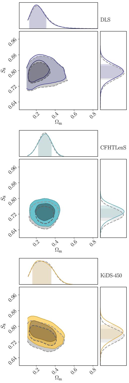
This plot illustrates the change in the cosmological constraints when we change the angular values used in the data vector: the grey dashed contour shows the constraints using the bin centres, while the coloured contour shows the constraints using the weighted centres.
APPENDIX B: THE KIDS-450 COVARIANCE
In Fig. B1, we show the effect of different approaches in marginalizing σm for the Baseline KiDS-450 case. For (1), we use the survey-provided covariance that includes σm. For (2) we use the survey-provided covariance without σm, and include σm using equation (12) of Hildebrandt et al. (2017). For (3), we use the survey-provided covariance without σm, and marginalize over σm at the parameter level. We find that (2) and (3) are in very good agreement, demonstrating that the two approaches are effectively equivalent, while (1) is shifted. The reason for the shift is due to the fact that (1) uses the noisy data vector in equation (12) of Hildebrandt et al. (2017), instead of a theoretical data vector. This is also explained in Troxel et al. (2018b).
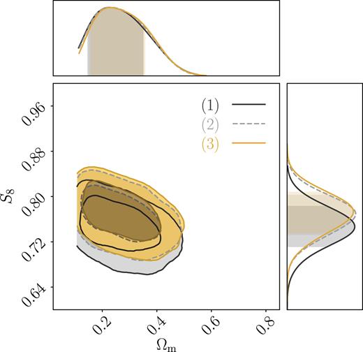
KiDS-450 constraints when using different approaches to marginalize σm.
APPENDIX C: SCALE CUT VALUES
In Table C1 we list the scale cuts used in Section 5.3. We also show the redshift |$z$|p used to calculate these scale cuts, as well as the number of data points remaining after making the scale cuts.
Top: The redshift of the peak of the lensing efficiency for each redshift bin in each survey. |$z$|p is used to calculate the scale cuts in the bottom table. Bottom: Scale cuts applied in each survey. Each row is for a combination of bins. The bins are ordered as (bin1, bin1), (bin1, bin2) ... (bin1, binN), (bin2, bin2) ... (bin2, binN) ... (binN, binN), where N is the maximum number of bins and binN is the highest redshift bin. The maximum scale cuts are fixed to the survey-specified scale cuts. ‘–’ indicates no data points are used after the scale cut. The last row lists the remaining number of data points after the scale cut.
| DLS | CFHTLenS | DES-SV | KiDS-450 | ||
|---|---|---|---|---|---|
| |$z$|p | bin1 | 0.13 | 0.13 | 0.19 | 0.13 |
| bin2 | 0.22 | 0.18 | 0.29 | 0.23 | |
| bin3 | 0.31 | 0.23 | 0.42 | 0.28 | |
| bin4 | 0.42 | 0.28 | 0.38 | ||
| bin5 | 0.57 | 0.38 | |||
| bin6 | 0.43 | ||||
| bin7 | 0.48 | ||||
| Conservative | |||||
| DLS | CFHTLenS | DES-SV | KiDS-450 | ||
| θmin, ± (arcmin) | 8.7/78.6 | 8.7/78.6 | 6.2/56.5 | 9.0/81.3 | |
| 8.7/78.6 | 8.7/78.6 | 6.2/56.5 | 9.0/81.3 | ||
| 8.7/78.6 | 8.7/78.6 | 6.2/56.5 | 9.0/81.3 | ||
| 8.7/78.6 | 8.7/78.6 | 4.6/41.6 | 9.0/81.3 | ||
| 8.7/78.6 | 8.7/78.6 | 4.6/41.6 | 5.6/50.4 | ||
| 5.7/51.3 | 8.7/78.6 | 3.6/33.0 | 5.6/50.4 | ||
| 5.7/51.3 | 8.7/78.6 | 5.6/50.4 | |||
| 5.7/51.3 | 6.6/60.0 | 4.8/43.5 | |||
| 5.7/51.3 | 6.6/60.0 | 4.8/43.5 | |||
| 4.4/40.0 | 6.6/60.0 | 3.9/35.4 | |||
| 4.4/40.0 | 6.6/60.0 | ||||
| 4.4/40.0 | 6.6/60.0 | ||||
| 3.6/33.0 | 6.6/60.0 | ||||
| 3.6/33.0 | 5.5/49.6 | ||||
| 3.1/28.0 | 5.5/49.6 | ||||
| 5.5/49.6 | |||||
| 5.5/49.6 | |||||
| 5.5/49.6 | |||||
| 4.8/43.0 | |||||
| 4.8/43.0 | |||||
| 4.8/43.0 | |||||
| 4.8/43.0 | |||||
| 3.9/35.1 | |||||
| 3.9/35.1 | |||||
| 3.9/35.1 | |||||
| 3.6/32.6 | |||||
| 3.6/32.6 | |||||
| 3.4/30.6 | |||||
| # of data points | 94 | 137 | 25 | 52 | |
| DLS | CFHTLenS | DES-SV | KiDS-450 | ||
|---|---|---|---|---|---|
| |$z$|p | bin1 | 0.13 | 0.13 | 0.19 | 0.13 |
| bin2 | 0.22 | 0.18 | 0.29 | 0.23 | |
| bin3 | 0.31 | 0.23 | 0.42 | 0.28 | |
| bin4 | 0.42 | 0.28 | 0.38 | ||
| bin5 | 0.57 | 0.38 | |||
| bin6 | 0.43 | ||||
| bin7 | 0.48 | ||||
| Conservative | |||||
| DLS | CFHTLenS | DES-SV | KiDS-450 | ||
| θmin, ± (arcmin) | 8.7/78.6 | 8.7/78.6 | 6.2/56.5 | 9.0/81.3 | |
| 8.7/78.6 | 8.7/78.6 | 6.2/56.5 | 9.0/81.3 | ||
| 8.7/78.6 | 8.7/78.6 | 6.2/56.5 | 9.0/81.3 | ||
| 8.7/78.6 | 8.7/78.6 | 4.6/41.6 | 9.0/81.3 | ||
| 8.7/78.6 | 8.7/78.6 | 4.6/41.6 | 5.6/50.4 | ||
| 5.7/51.3 | 8.7/78.6 | 3.6/33.0 | 5.6/50.4 | ||
| 5.7/51.3 | 8.7/78.6 | 5.6/50.4 | |||
| 5.7/51.3 | 6.6/60.0 | 4.8/43.5 | |||
| 5.7/51.3 | 6.6/60.0 | 4.8/43.5 | |||
| 4.4/40.0 | 6.6/60.0 | 3.9/35.4 | |||
| 4.4/40.0 | 6.6/60.0 | ||||
| 4.4/40.0 | 6.6/60.0 | ||||
| 3.6/33.0 | 6.6/60.0 | ||||
| 3.6/33.0 | 5.5/49.6 | ||||
| 3.1/28.0 | 5.5/49.6 | ||||
| 5.5/49.6 | |||||
| 5.5/49.6 | |||||
| 5.5/49.6 | |||||
| 4.8/43.0 | |||||
| 4.8/43.0 | |||||
| 4.8/43.0 | |||||
| 4.8/43.0 | |||||
| 3.9/35.1 | |||||
| 3.9/35.1 | |||||
| 3.9/35.1 | |||||
| 3.6/32.6 | |||||
| 3.6/32.6 | |||||
| 3.4/30.6 | |||||
| # of data points | 94 | 137 | 25 | 52 | |
