


ABSTRACT
Observational study of galactic magnetic fields is limited by projected observables. Comparison with numerical simulations is helpful to understand the real structures, and observational visualization of numerical data is an important task. Machida et al. (2018) have reported Faraday depth maps obtained from numerical simulations. They showed that the relation between azimuthal angle and Faraday depth depends on the inclination angle. In this paper, we investigate 100 MHz to 10 GHz radio synchrotron emission from spiral galaxies, using the data of global three-dimensional magnetohydrodynamic simulations. We model internal and external Faraday depolarization at small scales and assume a frequency-independent depolarization. It is found that the internal and external Faraday depolarization becomes comparable inside the disc and the dispersion of Faraday depth becomes about |$4\, {\rm rad\, m^{-2}}$| for face-on view and |$40\, {\rm rad\, m^{-2}}$| for edge-on view, respectively. The internal depolarization becomes ineffective in the halo. Because of the magnetic turbulence inside the disc, frequency-independent depolarization works well and the polarization degree becomes 0.3 at high frequency. When the observed frequency is in the 100 MHz band, polarized intensity vanishes in the disc, while that from the halo can be observed. Because the remaining component of polarized intensity is weak in the halo and the polarization degree is about a few per cent, it may be difficult to observe that component. These results indicate that the structures of global magnetic fields in spiral galaxies could be elucidated, if broad-band polarimetry such as that with the Square Kilometre Array is achieved.
1 INTRODUCTION
It is known that spiral galaxies have magnetic fields with strengths of a few |$\mu$|G on average (e.g. Soida et al. 2011), and the energy of the global, ordered magnetic field is comparable to the energy of the local, turbulent magnetic field. The global fields topologies of spiral galaxies have been studied using the relation between azimuthal direction and the Rotation Measure (RM), such as Axisymmetric Spiral and Bisymmetric Spiral (Fujimoto & Sawa 1987; Chiba & Tosa 1989; Krause ). The high spatial resolutions obtained with radio interferometric observations, such as with the Jansky Very Large Array (JVLA), allow observations of smaller scale components and investigation of the detail structures in RM (e.g. Beck 2015, and references therein). For example, the magnetic fields of M51 which has a clear grand-design spiral show a radial distribution 25–10|$\mu \, {\rm G}$| from centre to the outer edge (Fletcher et al. 2011). The structures of the halo magnetic fields are reported in face-ons/edge-ons (e.g. Krause 2014; Mulcahy, Beck & Heald 2017; Mulcahy et al. 2018). Maintaining such magnetic field strength in a normal spiral galaxy for billions of years requires a maintenance mechanism that acts against magnetic dissipation. As a model of the maintenance mechanism, Parker (1970) and Parker (1971) proposed a galactic dynamo that converts the kinetic energies of the galactic differential rotation and associated turbulent motion into magnetic energy. The galactic dynamo can amplify the initial weak seed magnetic field and maintains microgauss magnetic fields over 108 yr. Extended models based on galactic dynamo theory were proposed in the 1980s. One of the key constraints in the mean-field dynamo theory is the conservation of magnetic helicity (e.g. Blackman & Field 2001, and references therein). The growth of magnetic helicity of opposite signs between the large-scale and small-scale magnetic fields suppresses the dynamo action. The small-scale magnetic helicity fluxes should be removed to avoid the suppression and there are some candidate mechanisms such as advection of magnetic fields by outflow, turbulence produced by differential rotation and diffusion. In order to consider the effect of these process, recent theory of the mean field dynamo include the connection between disc and halo (Shukurov et al. 2006; Prasad & Mangalam 2016) which is considered to be the effect of the supernova explosions and magneto-rotational instability (MRI) (Balbus & Hawley 1991). They concluded that the growth rate of the turbulence by supernova explosions is faster than that of MRI. The explosions of the magnetic helicity make a corona which has a large-scale magnetic field. The magnetic field strength in the corona is much weaker than that in the disc.
However, these works do not consider the feedback of the magnetic fields and the influence of magnetic fields on the motion of the gas cannot be ignored (Balbus & Hawley 1991) in the diferentially rotating system. To build a galaxy model that takes into account the effects of magnetic fields on the gas motion, several global simulations of a galactic gas disc have been carried out (Nishikori et al. 2006; Hanasz et al. 2009; Machida et al. 2009, 2013). Machida et al. (2013) performed a three-dimensional magnetohydrodynamic (MHD) simulations of the galactic gas disc, and found that the evolution of the galactic disc can be described by the dynamo effect according to the MRI and Parker instability. As the MRI grows with the magnetic pressure reaching 10 per cent of the gas pressure, the azimuthal magnetic field is amplified. Then, where magnetic pressure reaches 20 per cent of the gas pressure, the magnetic flux gradually floats out from the disc due to the Parker instability. Since this flux lifting causes the dynamo action, the disc magnetic field is again amplified. Even if only weak magnetic field is assumed at the beginning, numerical results show global spiral magnetic arms with turbulence. The direction of the azimuthal magnetic field inverts quasi-periodically in both radial and vertical directions. The magnetic fields amplified inside the disc are supplied to the halo constantly. This mechanism has, however, not yet been proven by observations; it is still difficult to measure global magnetic fields in galaxies even with current large observational facilities such as the JVLA and LOFAR. Wideband and high spatial resolution observations with the Square Killometre Array (SKA) will reveal complex structures that reflect the MRI and Parker instability. Therefore, theoretical predictions prior to observations are important.
Machida et al. (2018) (hereafter Paper I) obtained Faraday depth (FD) maps and synchrotron intensity at high frequency using the results of Machida et al. (2013). It is found that the appearance of global magnetic field depends on the viewing angle; the magnetic fields appear as a hybrid type which consist of an axisymmetric spiral and higher modes for a face-on view, partially a ring-like structure at an inclination of ∼70°, and a structure parallel to the disc for the edge-on view. The magnetic vector seen at centimetre wavelengths traces the global magnetic field inside the disc.
In this paper, we investigate 100 MHz to 10 GHz radio synchrotron emission from spiral galaxies to provide a theoretical model of global magnetic fields in spiral galaxies. We aim to clarify the relation between projected observables and the actual three-dimensional structure of galactic magnetic fields using our sophisticated model. We would also like to clarify the effect of Faraday depolarization. We introduce the calculation method in Section 2. The numerical results are shown in Section 3, followed by discussion and summary in Sections 4 and 5, respectively.
2 OBSERVATIONAL VISUALIZATION
Global MHD simulation of a galactic gaseous disc by Machida et al. (2013) is adopted to our model galaxy, similar to Paper I. We adopted the cylindrical coordinate system (r, ϕ, |$z$|′). The simulated region is |$r\, {\rm kpc} \lt 56$| in the radial direction, |$|z^{\prime }|\, {\rm kpc} \lt 10$| in the vertical direction, and 0 ≤ ϕ ≤ 2π in the azimuthal direction. The spatial resolution where we focus on in this paper is Δr = 50 pc, Δ|$z$|′ = 10 pc, and Δϕ = 2π/256, respectively. The units of the numerical calculation such as the length, velocity, and density are |$r_0 = 1\, {\rm kmp}$|, |$v_0 = 207\, {\rm km\, s}^{-1}$|, and |$\rho _0 = 1\, {\rm cm^{-3}}$|, respectively. The unit of magnetic field strength is defined by the plasma β as |$B_0 = \sqrt{\rho _0 v_0^2}= 26 \mu \, {\rm G}$|. After the magnetic turbulence was amplified by MRI, the disc reached the quasi-steady state. At that time, the averaged density becomes |$0.01\, {\rm cm^{-3}}$| and magnetic field strength is about 5 |$\mu \, {\rm G}$|. The gas temperature inside the disc is about a few |$10^5 \, {\rm K}$| because the gas of the disc assumed the adiabatic. The plasma β ranges from about a few times 10−1 to 103. Only less than 1 per cent volume of the galactic disc has the low β (β < 5). Otherwise, the plasma β is typically 10–100 in the disc. The details of our numerical simulation are shown in Machida et al. (2013) and appendix A in Paper I.
The model galaxy is assumed an external galaxy and we calculate the Faraday rotation measure and the Stokes parameter of the radio band. Towards future radio polarimetry, we consider broad-band observations between 100 MHz and 10 GHz throughout the paper. Hereafter, we refer to the FD as a line-of-sight (LOS) integral of the LOS component of magnetic field weighted with the density, while RM is given by wavelength dependence of the polarization angle (PA).
The visualization of the simulation is a cube with size 20 kpc and coordinates (x, y, |$z$|) centred on the centre of the galaxy. We construct two-dimensional maps of 200 × 200 pixels centred on the projected centre of the galaxy, which results in an image resolution of 100 pc, corresponding to ∼2 arcsec for a galaxy in the Virgo cluster at a distance of ∼20 Mpc.
2.1 Model of depolarization
In the visualization, the spatial resolution of numerical data is the main factor of uncertainty. We cannot directly reproduce depolarization features (Burn 1966; Sokoloff et al. 1998; Arshakian & Beck 2011; Shneider et al. 2014) caused by structures below the resolution. Here, the frequency-independent depolarization determines the intrinsic polarization degree (PD), which can be parametrized using strengths of the mean and turbulent magnetic fields. The differential Faraday rotation depolarization primarily depends on mean LOS magnetic fields, whose effect can be naturally considered in numerical integration along the LOS, while an effect from unresolved turbulent LOS magnetic fields should be of a higher order. As for the beam depolarization, both internal and external Faraday dispersion depolarization caused by unresolved turbulent magnetic fields can be significant and we therefore describe it adequately.
Unless the resolution is much higher than the characteristic scale of turbulent magnetic fields, polarization will be underestimated because of significant Faraday dispersion depolarization on sub-resolution scales. Reproducing turbulence on a parsec scale, which is expected to be the characteristic scale in spiral arms (e.g. Haverkorn et al. 2006; Beck 2007), is however expensive for our simulation of a whole galaxy with a scale of a few tens of kpc. Therefore, visualization of global MHD simulation of spiral galaxies is essentially quite challenging, particularly at low frequencies.
In our numerical data, the azimuthal magnetic field power spectrum obeys the Kolmogorov law with a power-law index a ∼ −5/3 for wavenumbers n > 6. The spectra of the other field components and the gas density near the equatorial plane also indicate power-law spectra with an index −5/3 ≲ a ≲ −1 for n > 10. The simulation thus solved the forcing range and part of the inertial range of turbulence. Since the amplitude of the power spectrum is still enough values on smaller scale, the turbulence on smaller scale than the spatial resolution is considered assuming the Kolmogrov law. On the other hand, the power-law index for the halo components becomes smaller than that in the disc and significant peaks do not appear. Therefore, we adopt the laws of Faraday dispersion depolarization, and replace the dispersion of FD, σFD, for a certain image pixel into fluctuation of FDs around the pixel. This model makes an uncertainty on this work, which however is within a factor of about 2 (see Section 4.1).
2.2 Procedure of visualization
We assume that the cosmic-ray has equilibrium energy density with the magnetic energy. In order to obtain the number density of the cosmic-ray, we have assumed that the range of the Lorentz factor for cosmic-ray electrons is 200–3000 (Akahori et al. 2018). The energy spectral index p = 3 is adopted as a typical value (Sun et al. 2008).
3 RESULTS
Because the result of the simulation data we assumed is a similar data set of Paper I, the results at 8 GHz are same as that of Paper I. Below, we first determine the fiducial unit density of the MHD simulation data, and then show the results of face-on view and edge-on view.
3.1 Determination of the fiducial unit density
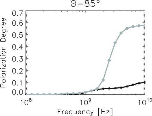
In our MHD simulation data, because the density is a free parameter, we can assume its value freely. And the magnetic field strength and the synchrotron intensity strongly depend on the unit density of the data. Therefore, we check the dependence of the unit density for the observables and determine the fiducial unit density we assumed. Fig. 1 shows the dependence of the PD on the unit density. As representative cases, we chose an arm region for an inclination angle of 5° at (1.5 kpc, 0 kpc) and a disc region for an inclination angle of 85° at (3 kpc, 0 kpc). The PDs in this panel is measured on one pixel. The symbols denote the cases with different unit densities; they increase from left to right.
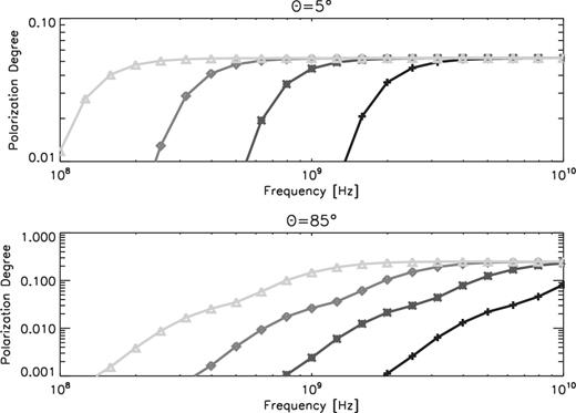
PDs of the emission from an arm region for the inclination angle of 5° (nealy face-on, top panel) and from a disc region for the inclination angle of 85° (nearly edge-on, bottom panel), as a function of the frequency. The symbols denote the cases with different unit densities: |$3\times 10^{-3}\, \rm {cm}^{-3}$| (triangle), |$0.01\, \rm {cm}^{-3}$| (diamond), |$0.03\, \rm {cm}^{-3}$| (cross), and |$0.1\, \rm {cm}^{-3}$| (plus).
According to the previous radio observations introduced in Section 1, PDs of less than 5 per cent were observed at frequencies lower than 1 GHz in face-on galaxies, and no polarization was detected at 151 MHz in M51 (Fletcher et al. 2011; Mulcahy et al. 2014). In edge-on galaxies, the typical degree of polarization at 1 GHz is a few per cent in the disc and increases to 10–20 per cent in the halo (see e.g. Hummel, Beck & Dahlem 1991). At 146 MHz, no polarization was detected in NGC 891 with LOFAR (Mulcahy et al. 2018). The case with |$0.03\, \rm {cm}^{-3}$| fits with the observations therefore we choose |$0.03\, \rm {cm}^{-3}$| as the fiducial unit density in this paper. Indeed, with the unit density of |$0.03\, \rm {cm}^{-3}$|, the average thermal electron density in the disc is |${\sim } 0.03\, \, {\rm cm^{-3}}$| and that in the halo is |${\sim } 3 \times 10^{-4}\, \, {\rm cm^{-3}}$| which are consistent with X-ray observations of a hot disc (Sakai et al. 2014).
The FD contour maps (Fig. 2a and Fig. 3a in Paper I) have an upper and lower limit and the range of FD value is wide. The low FD region is difficult to find out, because the contrast of the FD around |$0\, \, {\rm rad \, m^{-2}}$| is too weak to identify. Therefore, we show the histogram of the FDs. Fig. 2 shows the volume filling factor of FD. The black and grey histogram show the results for inclinations of 5° and 85°, respectively. The horizontal axis shows FD. The most volume zone of FD for the case of 5° is 0.3 from 5 |$\, {\rm rad \, m^{-2}}$| to 10 |$\, {\rm rad \, m^{-2}}$|. Although one of the volume zone for model 85° is from 5 |$\, {\rm rad \, m^{-2}}$| to 10 |$\, {\rm rad \, m^{-2}}$|, |FD| > 100 |$\, {\rm rad \, m^{-2}}$| also have 0.15. These region whose absolute value of FD becomes greater than 100 |$\, {\rm rad \, m^{-2}}$| corresponds to the halo and |FD|<20 |$\, {\rm rad \, m^{-2}}$| region is the result from the disc. The corresponding average magnetic field strength both of disc and halo is about 10 |$\mu \, {\rm G}$|.
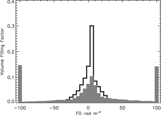
The volume filling factor of FD. The black and grey histogram show the results in the case of 5° and 85°, respectively. The horizontal axis shows FD.
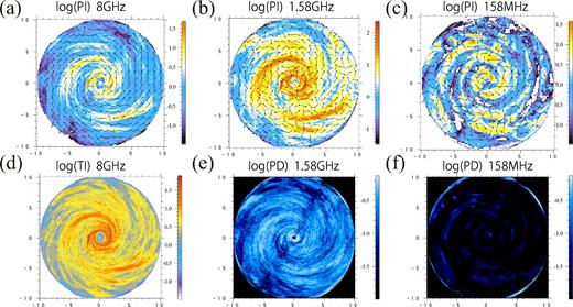
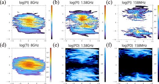
(a), (b), (c): Simulated polarized intensity for face-on view at the observed frequencies of 8 GHz, 1.58 GHz, and 158 MHz, respectively, all in units of |$\mu$|Jy beam−1. The arrows indicate the magnetic vector (2χ + 90°) which has constant length and hence only denotes the direction of the magnetic fields. (d): Simulated synchrotron total intensity at the observed frequency of 8 GHz. (e), (f): Polarization degree at the observed frequency of 1.58 GHz and 158 MHz, respectively.
3.2 Face-on view
Polarized intensity (PI) plots are shown in Fig. 3a, 3b, and 3c at the observed frequency of 8 GHz, 1.58 GHz, and 158 MHz, respectively. Fig. 3d shows total synchrotron intensity (TI) at the observed frequency of 8 GHz. The arrows show the magnetic vector, 2χ + 90°, with χ obtained from the Stokes Q and U (equation12), whose direction only have a meaning. PDs at frequencies of 1.58 GHz and 158 MHz are shown in Figs 3e and 3f, respectively. As we have already shown in Paper I, TI and PI (8 GHz) reflect the spiral magnetic field structure inside the gas disc. The result of the model that mean fields are stronger in the arms than in the inter-arm regions is different from observations in grand-design galaxies having strong density waves (Fletcher et al. 2011), but such galaxies are beyond the scope of the MRI model, as mentioned in Paper I.
However, the spiral pattern becomes different at lower frequencies. That is, anti-correlation between TI and PI is found in PI(158 MHz); TI is stronger but PI is weaker at (1.5 kpc, 0 kpc), and TI is weaker but PI is stronger at (2 kpc, 6 kpc). The polarization degree (PD = PI/TI) distribution (Fig. 3e) is not uniform; PD becomes small where TI is relatively large and PD gradually increases at the edges of regions of strong TI. The depolarization becomes more important near the galactic centre owing to the higher density and stronger magnetic field. The PD inside the magnetic spiral arms becomes under 1 per cent. According of these effects, the high PI regions at 158 MHz trace the spiral magnetic field in the halo. As for the PI at 1.58 GHz, the spiral pattern becomes close to that of TI, but the polarized vector rotates significantly, particularly around the disc spiral arms at which the FD is about 20–40 rad m−2. These features can be ascribed to depolarization and Faraday rotation. The maximum value of the PI at 158 MHz is similar to that at 8 GHz, although the positions of PI peak are different between them. The PI at the magnetic spiral arms attains the highest value at high frequency, because the intensity becomes highest and Faraday depolarization does not work in such a high-frequency region. On the other hand, when the observed frequency is 100 MHz bands, the peak position of the PI move to the surrounding region of the magnetic spiral arm. It is because Faraday depolarization occurs in the arm region and PI decreases in the arm region. The peak intensity of PI increases from 8 GHz to 1 GHz, and it reduces from 1 GHz to 100 MHz. Although an increase of PI from 8 GHz to 1 GHz was observed in the outer regions of some face-on galaxies, the PI in the inner disc decreased (Beck 2007; Fletcher et al. 2011). This is because the amount of Faraday depolarization computed in our calculation may be underestimated; the density around the central region is lower than that seen in the real spiral galaxies because the galaxy model we used have adopted an absorption boundary condition inside 200 pc. The reason we adopted the absorption boundary is that the in-falling matter heats up the central region.
Fig. 4 shows the frequency dependence of the PD. The black and grey curves show the result in the spiral arm and in the inter-arm region. The PD is calculated for one pixel at (1.5 kpc, 0 kpc) in the arm region and (0 kpc, 1.5 kpc) in the inter-arm region. Indeed, the PD decreases below a few GHz, which corresponds to FD of dozens rad m−2 according to Faraday dispersion depolarization (Arshakian & Beck 2011). Below a few MHz, the PD becomes less than 0.1. Because of the effect of frequency-independent Faraday depolarization, the maximum PD becomes about 0.35 in the arm and 0.2 in the inter-arm. Although turbulent components inside the arm and inter-arm are of similar strength, mean components whose direction turns to the same direction in the arm region become larger than the inter-arm region. Therefore, frequency-independent depolarization in the arm becomes smaller than that of the inter-arm and the saturation value of PD in the arm becomes larger than the value in the inter-arm region.
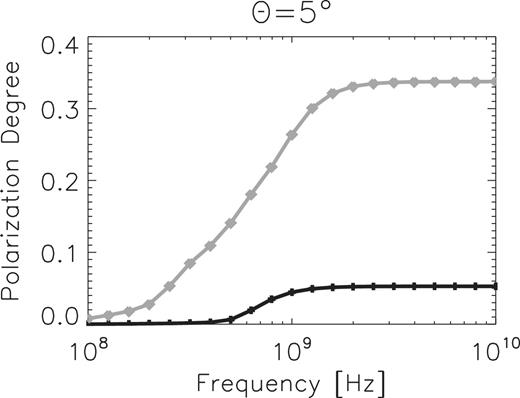
PDs of the emissions from an arm (x, y) = (1.5 kpc, 0.0 kpc) (black line with crosses) and from an inter-arm (0 kpc, 1.5 kpc) (grey line with asterisks) of θ = 5°, as a function of the frequency.
3.3 Edge-on view
Figs 5a, 5b, 5c, 5d, 5e, and 5f show the maps of PI(8 GHz), PI(1.58 GHz), PI(158 MHz), TI(8 GHz), PD(1.58 GHz), and PD(158 MHz), respectively. Overall, TI becomes larger towards the galactic mid-plane, because the global magnetic field is strongest in the disc. Structures seen in PI(8 GHz) are similar to those seen in TI, and the magnetic vector nicely traces the global azimuthal magnetic field. Such similarity is completely missing in low frequencies. At 158 MHz, PI is seen mostly in the halo in spite of strong magnetic fields in the disc. The direction of magnetic vectors becomes vertical as a result of Faraday rotation. The shape of PI(1.58 GHz) looks like an hourglass due to depolarization around the disc. The PD(158 MHz) becomes less than 10−3 even in the halo. Overall, the nature of these features is the same as that seen in the face-on view.
Same as Fig. 3 but for θ = 85°.
Fig. 6 shows the frequency dependence of the PD. For the LOS towards the disc (3 kpc, 0 kpc) for one pixel, depolarization is significant in all frequency ranges considered; the PD at 10 GHz becomes under 0.1 due to frequency-independent depolarization. The PD falls much below 0.1 at a frequency below 1 GHz due mostly to the external Faraday dispersion depolarization.
PDs of the emissions from a disc (3 kpc, 0 kpc) (black line with crosses) and from a halo (−3 kpc, 3 kpc) (grey line with asterisks) of θ = 5°, as a function of frequency.
Meanwhile, for the LOS towards the halo (3 kpc, 3 kpc), depolarization becomes important only below a few hundred MHz. This is due to the fact that the FD (and the standard deviation of the FD) is small because of the low density in the halo. The high saturation values of PD above 2 GHz in the halo indicate that the mean fields become dominant, because of the outflow from the galactic disc.
Because the global azimuthal magnetic field becomes less important at low frequencies, PI(158 MHz) unveils secondary components of magnetic fields. For instance, the magnetic vector seems to be random, tracing not the global azimuthal magnetic field but the turbulent magnetic field. Actually, the power spectrum of magnetic fields in the halo is almost a power law at n > 2, meaning that the halo magnetic field is turbulent. It is also interesting that, around the rotation axis of the galaxy, the magnetic vector partly traces the global vertical magnetic field and points towards the vertical direction.
4 DISCUSSION
4.1 Uncertainty of visualization
We have conducted observational visualization of disc galaxies using the data of numerical simulations for galactic gaseous discs. Looking forward to future broad-band radio polarimetry, we have attempted to reproduce observables in a very wide range of frequencies between 100 MHz and 10 GHz. It is difficult to handle depolarization effects at small spatial scales, and we have adopted a model that assumes that the power of turbulent magnetic field within the spatial resolution can be replaced with that around the resolution. This adds an uncertainty to our visualization of observables at low frequencies.
In order to estimate the uncertainty on the model, we performed independent simulations of FD maps. We made an FD map of 1 kpc2 with 5002 pixels (so that the pixel resolution is 2 pc). The FD map contains Kolmogorov turbulence with an average and standard deviation of 0 |$\, {\rm rad \, m^{-2}}$| and 10 |$\, {\rm rad \, m^{-2}}$|, respectively. A 100 pc2 box (the same as the resolution of our work) at the centre is chosen to derive the standard deviation of FD, σFD, actual. We also calculate the average FDs of eight boxes around the central box (see the left-hand panel of Fig. 7) and derive the standard deviation of the averages, σFD, model. The comparison between σFD, actual and σFD, model for 100 realizations is shown in the right-hand panel of Fig. 7. Although there is variance between the runs, the average σFD, actual and σFD, model are ∼5.0 and ∼9.6, respectively. Therefore, the model can estimate the standard deviation within a factor of about 2. We leave this offset in this work, since the value highly depends on the actual magnetic field power spectrum.
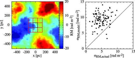
(Left) An example of a 5002 pixel FD map showing Kolmogorov turbulence. The black box is used to calculate σFD, actual, while σFD, model is evaluated in the red boxes (see the text). (Right) Comparison between σFD, actual and σFD, model. The results for 100 realization simulations are shown.
Another uncertainty in our visualization is caused by numerical interpolation (averaging) around the resolution. When we obtained the average and turbulent components of FD by equations (1) and (2), we adopted the average of magnetic fields inside the ±N + 1 cells. We have checked the dependence of the results on N by varying N = 0, 1, 3, 5, 6, 10, where N = 0 means the interpolation with the nearest eight cells in the cylindrical coordinate data set. For a physical value along the LOS of the i-th pixel (Xi), the results with N = 0 and N = 1 are similar to each other. N = 6 makes the power spectrum at n > 30 steeper, and N = 10 almost cancels out turbulent components. As for an average |$X_{\, {\rm ave},i}$| derived with Xj of eight pixels around the i-th pixel, N = 3 and N = 6 produce similar results to each other. Based on these studies, we decided to adopt N = 0 in X and N = 5 in Xave.
4.2 Dependence of the unit density
In the previous section, we presented the results with a fiducial unit density (ρ0 = 0.03 |$\, {\rm cm^{-3}}$|), whose PDs in 100 MHz bands are still higher than the observational results (Mulcahy et al. 2014, 2018). It is also useful to study the cases with lower and higher unit densities, which could be compared to the spiral galaxies, respectively. Fig. 8 shows the results with the lower (|$0.3\, \rho _0$|, left-hand panels) and higher (|$3\, \rho _0$|, right-hand panels) unit densities.
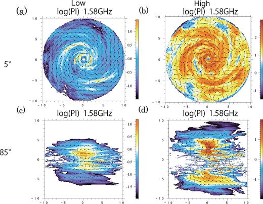
PI maps at 1.58 GHz. Left-hand and right-hand panels show the results of the lower (|$0.3\, \rho _0$|) and higher (|$3\, \rho _0$|) unit densities, respectively, where ρ0 = 0.03 |$\, {\rm cm^{-3}}$|. The top and bottom panels show the cases for θ = 5° and 85°, respectively.
In the lower case, structures of PI(1.58 GHz) for 5° (Fig. 8a) and for 85° (Fig. 8c) are broadly consistent with those of PI(8 GHz) with the fiducial unit density, Fig. 3b and Fig. 5b, respectively. This indicates one to one correspondence with FD (or σFD) and the wavelength squared (e.g. equations 6, 7, 12). In the higher case, structures of PI (1.58 GHz) for 5° (Fig. 8b) and for 85° (Fig. 8d) are broadly consistent with those of PI (1.58 GHz) with the fiducial unit density, Fig. 3b and Fig. 5b, respectively, except a bit stronger depolarization towards the disc plane for 85°. Clear difference between the fiducial and higher unit densities is the magnetic vector; the higher case shows more random magnetic vectors due to the Faraday rotation. The high case of 85° shows the hourglass distribution and vertical magnetic vectors around the rotation axis. These structures are observed in edge-on galaxies around 1.4–4.8 GHz. Because the magnetic energy in the halo region is half of that in the disc, PI shows the characteristic feature around the rotation axis. Because the magnetic field strength is proportional to the number density, the strength of the PI depends on the 1.5 square of the density. And the PI becomes five times larger than the fiducial model. Therefore, the PI in the high-latitude region becomes bright in high-density model.
4.3 LOS distribution of the dispersion of FD
Fig. 9a shows the distribution of the FD dispersion along the LOS for the 5° inclined model. The black and grey curves show the |$\sigma _{\, {\rm FD}, i, k}$| and |$\sigma _{\, {\rm FD}, i, l}$|, respectively. The top and bottom panels show the results at (2 kpc, −0.5 kpc), and (3 kpc, 0 kpc), respectively. The effect of the internal depolarization shows a similar tendency and the averaged values of σFD, l in the disc is about 4 |$\, {\rm rad \, m^{-2}}$| both in the arm and the inter-arm. On the other hand, the effect of the external depolarization is different in the arm and the inter-arm. |$\sigma _{\, {\rm FD}, k}$| in the arm is comparable to the |$\sigma _{\, {\rm FD},l}$|. Because of the mean fields, FDs have similar values in the arm. Therefore, |$\sigma _{\, {\rm FD},k}$| becomes small in the arm. The turbulent component is dominant in the inter-arm, however, FD in the inter-arm is smaller than that in the arm and can have various values. Then |$\sigma _{\, {\rm FD},k}$| becomes large. When LOS goes to the opposite side of the equatorial plane, the values of FD becomes small because of the low density. Therefore, the effect of the internal depolarization becomes important inside the galactic disc. The top and bottom panels of Fig. 9b show the results at (3 kpc, 0 kpc) and (3 kpc, 3 kpc) for the 85° inclined model, respectively, which correspond to disc and halo. The averaged value of |$\sigma _{\, {\rm FD}, k}$| and |$\sigma _{\, {\rm FD},l}$| in the disc is about |$200\, \, {\rm rad \, m^{-2}}$| and |$40\, \, {\rm rad \, m^{-2}}$|, respectively. In the edge-on case, the toroidal components, which are the dominant components of the magnetic field in the system, become the main components of the LOS fields. Since the turbulent components of the toroidal (azimuthal) magnetic fields are stronger than the mean fields, the mean fields becomes 70 per cent of the toroidal fields. Therefore, the effect of the internal depolarization becomes smaller than that in the face-on case.
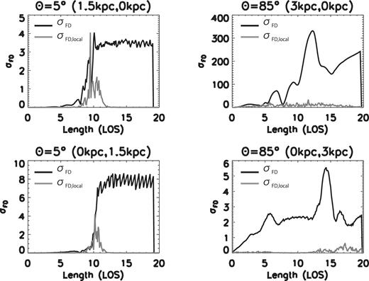
Distribution of the FD dispersion along the LOS. The black and grey curves show the |$\sigma _{\, {\rm FD},i,k}$| and |$\sigma _{\, {\rm FD},i,l}$|. (a) The top and bottom panels denote the values in the arm and inter-arm region for inclination angle θ = 5°. (b) The top and bottom panels show the values in disc and halo for inclination angle θ = 85°.
4.4 Can PI at MHz-band be observed or not?
Fig. 10 shows the PI at the observing frequency of 158 MHz masked where PD <0.01. Because Faraday depolarization works effectively in magnetic spiral arms, PD in the arm becomes lower than 0.01 in the case of 5°. The remaining PI components are created in the halo and maximum strength of PI is 38 |$\mu \, {\rm Jy\,beam^{ -1}}$| (Fig. 10a). On the other hand, in the case of 85°, PI remained around the rotational axis and its strength is less than |$10 \mu \, {\rm Jy\,beam^{ -1}}$|.
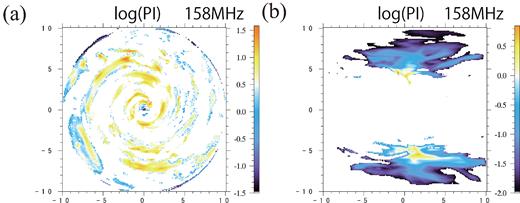
PI maps masked where PD is over 0.01. (a) θ = 5°, (b) θ = 85°.
5 SUMMARY
We summarize the points discussed in this work.
TI and PI (>4 GHz) are both stronger along denser magnetic spiral arms, where depolarization is insignificant at such high frequencies. The PA traces that of the azimuthal magnetic field inside the disc. Meanwhile, PI (<1 GHz) through the disc weakens due to depolarization. Note that the maximum values of PI(>158 MHz) and PI(>8 GHz) are similar to each other, though they appear at different places. An increase of PI from 8 GHz to 1 GHz is shown in our pseudo observations in the whole disc, although such increase was observed only in the regions of some face-on galaxies. This result may suggest that the depolarization effect in our model is underestimated for the real galaxies.
PI(158 MHz) through the magnetic spiral arms is faint. This is because depolarization significantly occurs due to large FD. Consequently, PI at such low frequencies traces the magnetic field structure in the halo. These tendencies do not depend on the inclination angle of the galaxy. The high PI(158 MHz) in the edge-on view traces the halo magnetic field formed by the intermittent emerging of magnetic flux produced by the Parker instability.
When the inclination angle is 5°, because the local FD dispersion inside the disc has a similar value to the FD dispersion, the effect of the internal Faraday depolarization becomes important inside the disc. On the other hand, in the case of 85°, FD dispersion becomes over 10 times larger than the local FD dispersion.
In this paper, we did not employ Faraday tomography, which is clearly complementary to our work and may be more powerful to deproject the LOS structure. It is, however, not trivial so far how we can translate the Faraday spectrum into real three-dimensional structure of the galaxy (Ideguchi et al. 2014). We need further studies of both observational visualization and Faraday tomography for numerical data.
ACKNOWLEDGEMENTS
We are grateful to Dr. R. Matsumoto, Dr. K. Takahashi, and Dr. S. Ideguchi for useful discussion. We also thank the anonymous referee for his/her useful comments and constructive suggestions. Numerical computations were carried out on SX-9 and XC30 at the Center for Computational Astrophysics, CfCA of National Astronomical Observatory of Japan (P.I. MM). A part of this research used computational resources of the High Performance Computing Interstructure (HPCI) system provided by FX10 of Kyushu University through the HPCI System Research Project (Project ID:hp140170). This work is financially supported in part by a Grant-in-Aid for Scientific Research (KAKENHI) from JSPS (P.I. MM:23740153, 16H03954, TA:15K17614, 15H03639).
