


Abstract
Recent multiband variability studies have revealed that active galactic nucleus (AGN) accretion disc sizes are generally larger than the predictions of the classical thin disc by a factor of 2 ∼ 3. This hints at some missing key ingredient in the classical thin disc theory: here, we propose an accretion disc wind. For a given bolometric luminosity, in the outer part of an accretion disc, the effective temperature in the wind case is higher than that in the no-wind one; meanwhile, the radial temperature profile of the wind case is shallower than the no-wind one. In presence of winds, for a given band, blackbody emission from large radii can contribute more to the observed luminosity than the no-wind case. Therefore, the disc sizes of the wind case can be larger than those of the no-wind case. We demonstrate that a model with the accretion rate scaling as |$\skew4\dot{M}_0 (R/R_{\mathrm{S}})^{\beta }$| (i.e. the accretion rate declines with decreasing radius due to winds) can match both the interband time lags and the spectral energy distribution of NGC 5548. Our model can also explain the interband time lags of other sources. Therefore, our model can help decipher current and future continuum reverberation mapping observations.
1 INTRODUCTION
The cross-correlation between two light curves of active galactic nucleus (AGN) continuum emission can provide model-independent constraints on the accretion disc sizes. The interband correlations might be caused by X-ray (e.g. Krolik et al. 1991) or far-ultraviolet (FUV) reprocessing (Gardner & Done 2017). According to the reprocessing scenario, X-ray or FUV emission acts as an external energy source (in addition to the internal viscous dissipation) and heats the outer accretion disc. As a result, emission at longer wavelengths (e.g. UV, optical and infrared (IR)) varies in response to X-ray or FUV variations (i.e. the ‘driving light curves’) after a light-traveltime delay (i.e. continuum reverberation mapping). Therefore, the interband time lags can be used to test the accretion disc theory. However, the observed interband time lags appear to be incompatible with the classical thin disc theory of Shakura & Sunyaev (1973). Indeed, the observed accretion disc sizes are 2 ∼ 3 times larger than the theoretical expectations (e.g. Edelson et al. 2015; Fausnaugh et al. 2016; Edelson et al. 2017; Jiang et al. 2017; Mudd et al. 2017; Starkey et al. 2017; Kokubo 2018; McHardy et al. 2018). Accretion disc sizes inferred from microlensing observations of quasars are also larger than expected (e.g. Morgan et al. 2010). These observational results indicate that some key ingredient is missing in the classical thin disc theory.
Several scenarios have been proposed to explain the larger-than-expected accretion disc sizes. For instance, Dexter & Agol (2011) suggested that an inhomogeneous accretion disc with temperature fluctuations can explain the microlensing results (for alternative explanations, see Abolmasov & Shakura 2012; Li, Yuan & Dai 2018). With some further modifications, this model can also explain the time-scale-dependent colour variations (Cai et al. 2016; Zhu et al. 2017). However, this model cannot explain interband time lags unless a speculative common large-scale temperature fluctuation is assumed to simultaneously operate over every part of the accretion disc (Cai et al. 2018). Gardner & Done (2017) argued that the observed interband time lags are not the simple light-travel time-scales but correspond to other physical time-scales (e.g. the dynamical or thermal time-scales). It is also speculated that the larger-than-expected time lags are caused by contribution of diffuse continuum emission from broad emission line (BEL) region (Cackett et al. 2017; McHardy et al. 2018). Last but not least, a non-blackbody disc due to electron scattering in the disc atmosphere can be used to explain the observed time lags; however, such a disc emits too much soft X-ray emission (Hall, Sarrouh & Horne 2018).
Here, we propose an alternative model to explain the larger-than-expected accretion disc sizes: an accretion disc suffers from significant winds. Winds, which can be probed by blueshifted absorption line features (or blueshifted emission lines; see e.g. Richards et al. 2011; Sulentic et al. 2017; Sun et al. 2018c) in X-ray (i.e. ultrafast outflows, warm absorbers; see Tombesi et al. 2013, and references therein), UV and optical bands (e.g. Weymann et al. 1991; Murray et al. 1995; Trump et al. 2006; Filiz Ak et al. 2014; Grier et al. 2015), are presumably common in AGNs and might be responsible for the scaling relations between supermassive black holes (SMBHs) and their host galaxies (i.e. AGN feedback; e.g. Fabian 2012; King & Pounds 2015). To emit the same bolometric luminosity (Lbol), the effective temperature of the disc is higher with significant winds than without except for the innermost part (see Fig. 1). In the presence of winds, the radial temperature profile is shallower than the classical T(R) ∝ R−3/4 law. As a result, for a given band, blackbody emission from large radii can contribute significantly to the total luminosity. Therefore, the accretion disc sizes inferred from interband time lags are larger than those of the classical disc model.

The radial distribution of effective temperature (Teff) for cases with the wind parameter β = 0.3 (solid line) and β = 0 (i.e. no wind; dashed line), respectively. The two discs emit the same bolometric luminosity (i.e. Lbol = 0.1LEdd); MBH is 8 × 10⁷ M⊙. At outer radii (i.e. r > 10), the effective temperature Teff for the wind case is larger than that for the no-wind case.
This work is formatted as follows. In Section 2, we explain our model in detail and explore the interband time lags of NGC 5548. We discuss our results in Section 3. We adopt a flat ΛCDM cosmology with h0 = 0.7 and ΩM = 0.3.
2 THIN DISC WITH WINDS
2.1 General arguments
We consider that the thin disc suffers from significant winds with a radius-dependent mass accretion rate, i.e. |$\skew4\dot{M}$| is a function of radius (R). Several mechanisms, including line-driving, radiation pressure, and magnetohydrodynamic acceleration, have been proposed to accelerate accretion-disc winds. The observed winds are unlikely to be driven by one universal mechanism; instead, different mechanisms might work on different spatial scales and different ionization states (for a review, see e.g. Proga 2007). For instance, the line-driving mechanism is likely to be efficient on scales of ≳300 RS (RS = 2GMBH/c2, where G, MBH, and c are the gravitational constant, black hole mass, and speed of light, respectively) and for the gas in a low-ionization state (e.g. beyond some ‘shielding’ gas that blocks X-ray photons; see e.g. Murray et al. 1995; Proga & Kallman 2004; Higginbottom et al. 2014). We are interested in winds that are launched from the inner most stable circular orbit (ISCO) to a few thousand RS. On such spatial scales, the line-driven mechanism is likely to be inefficient since gas at these small radii is unlikely to be shielded. Instead, magnetohydrodynamic acceleration is a promising alternative mechanism (e.g. Blandford & Payne 1982; Cao & Spruit 2013; Fukumura et al. 2014).
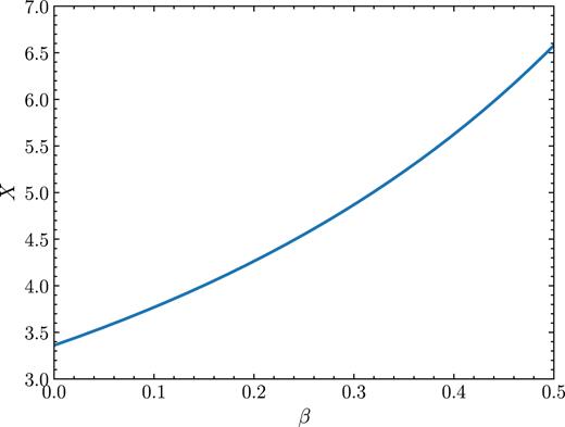
The ratio of the flux-weighted flux radius to the peak temperature radius X = Rfl/Rλ as a function of the wind parameter β (equation 7).
2.2 The slope of the time lag–wavelength relation
For a temperature profile of Teff ∝ λ−α, the time lag–wavelength relation should be τ ∝ λ1/α if the light curve is infinitely long and the accretion disc has a rather large outer boundary (e.g. 105 RS). That is, the slope of the time lag–wavelength relation for our windy disc is expected to be 4/(3 − β) (see equations 4 and 5). However, the observed slope can be different from 4/(3 − β) because of a few reasons. First, the outer boundary sets an upper limit (i.e. Rout/c) for the interband time lag. If the IR emission regions are close to the outer boundary, the time lag of IR emission with respect to UV emission increases slower than the τ ∝ λ4/(3 − β) relation. Second, the lag estimate is often subject to a large variance because of finite-duration monitoring and long-time-scale trends (Welsh 1999). Third, the induced temperature variations might not be very small. Under such circumstances, the temperature profile can be altered by the temperature variability. Note that a not-so-small temperature variation does not necessarily conflict with the observed small variability amplitudes of UV-Optical-IR emission. This is because the observed UV-Optical-IR emission is an integration of blackbody radiation of multiple emission regions; the integration process suppresses the variability. Without reprocessing simulations to account for such variance, it is inappropriate to infer temperature profile from the time lag–wavelength relation derived with short (∼102 d) light curves. Indeed, as we will show in Section 2.3 and Fig. 3, the slope varies significantly per each simulation and the slope of the median of the time lag–wavelength relation is actually shallower than 4/(3 − β).
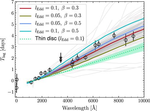
Time lag (with respect to the 1367 Å continuum) as a function of rest-frame wavelength for NGC 5548 (Edelson et al. 2015; Fausnaugh et al. 2016). The two star symbols denote the time lags of u and U bands; they are outliers since the two bands are significantly contaminated by BEL emission (Fausnaugh et al. 2016). Each of the 256 X-ray reprocessing simulations for the wind case with β = 0.3 and lEdd = 0.1 is shown as a grey solid curve. Due to reasons outlined in Section 2.2, the time lag–wavelength relation varies per simulation. The red thick solid curve represents the median time lag–wavelength relation of the 256 simulations. The remaining three thick solid curves indicate the median time lag–wavelength relations for other wind cases. For comparison, we also show the reprocessing of a classical thin disc with the same bolometric luminosity (the dotted curve; the shaded region indicates the 1σ uncertainties derived from the 256 simulations).
2.3 NGC 5548 as a test case
To compare our model with the observed interband time lags of NGC 5548, we model a thin disc with winds; the physical parameters are MBH = 8 × 10⁷ M⊙ (see Bentz et al. 2010; Pei et al. 2017) and the redshift |$z$| = 0.017175 (De Rosa et al. 2015). The inclination angle is unknown; we choose a representative value of i = π/4. The SMBH is assumed to be a non-spinning Schwarzschild black hole. The inner and outer boundaries of the thin disc are 3 RS and 2000 RS, respectively. As for the wind parameter β, we test two cases, β = 0.3 and β = 0.5. |$\skew4\dot{M}_0$| is selected in such a way that Lbol = lEddLEdd, where LEdd = 1.26 × 1038MBH/M⊙ erg s−1. We also test two cases for lEdd, lEdd = 0.05 and lEdd = 0.1. Therefore, we explore four cases: lEdd = 0.05 and β = 0.3; lEdd = 0.05 and β = 0.5; lEdd = 0.1 and β = 0.3; lEdd = 0.1 and β = 0.5.
This disc is illuminated with a driving light curve; the emission region of the driving light curve is assumed to be a point source located above the SMBH with a scale height of H = 5 RS. It is argued that the observed X-ray light curves are not consistent with the driving light curve (Gardner & Done 2017; Starkey et al. 2017, but see Sun et al. 2018b). Therefore, we assume the driving light curve and the 1367 Å light curve are similar. The external heating due to the driving light-curve illumination at each radius is assumed to be 1/3 of the internal viscous dissipation rate (Fausnaugh et al. 2016).
In Fig. 3, we show the time lag as a function of wavelength for our four cases. In near-IR bands, the relation is shallower because the outer boundary of the disc, which is fixed to 2000 RS, limits the time lags (i.e. equation 7 overpredicts X).6 Due to reasons outlined in Section 2.2, for fixed physical parameters (i.e. β, lEdd, MBH, i and inner and outer boundaries), the time lag–wavelength relation varies per simulation (the grey curves represent the 256 simulations for β = 0.3 and lEdd = 0.1). We then calculate the median time lag–wavelength relations (i.e. the thick solid curves). For β = 0.3 and lEdd = 0.1, the slope of the median relation is 1.12 ± 0.15, which is shallower than 4/(3 − 0.3) = 1.48; this case can fit the observed UV-optical-IR time lags reasonably well. Meanwhile, the case with β = 0.5 and lEdd = 0.05 can also explain the observed UV-optical-IR time lags. If we increase/decrease β or lEdd, the interband time lags will be larger/smaller. The case with β = 0.5 and lEdd = 0.1 (β = 0.3 and lEdd = 0.05) over(under)predicts the UV-optical-IR time lags by an overall factor of ∼1.2.
We can calculate the spectral energy distribution (SED) of a disc that suffers from winds by simply integrating the blackbody emission of the temperature profile of equation (4) over the whole accretion disc. In Fig. 4, we plot the luminosity density Lν versus λ from our models (the thick solid curves). The cases with β = 0.3 and lEdd = 0.1 or β = 0.5 and lEdd = 0.05 overpredict the optical-IR-UV emission by a factor of 2 ∼ 5 (the upper left-hand panel of Fig. 4).
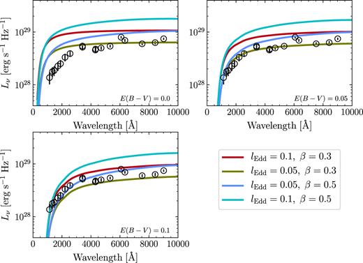
Broad-band SED of NGC 5548 from Fausnaugh et al. (2016), which is corrected for Galactic extinction with a Milky Way extinction law (Cardelli, Clayton & Mathis 1989) and E(B − V) = 0.0171 mag (Schlafly & Finkbeiner 2011). The solid curves indicate the SEDs derived from our disc-with-wind models. Without intrinsic extinction, these SEDs (the upper left-hand panel) generally overpredict the observations. However, such a discrepancy can be reduced if the SED has SMC-like intrinsic extinction. For E(B − V) = 0.05 and 0.1 mag, the resulting SEDs are presented in the upper right-hand and lower left-hand panels, respectively.
It has been demonstrated that the classical thin disc with multitemperature blackbody emission cannot fit all AGNs; additional modifications should be applied, including the disc wind and intrinsic extinction (Capellupo et al. 2015). In this work, the disc wind has been considered. The intrinsic extinction of NGC 5548 is not reliably determined. However, there is evidence that the intrinsic extinction is significant. For instance, Wamsteker et al. (1990) argue that an extinction level of E(B − V) = 0.05 mag exists. Meanwhile, the Balmer decrement of NGC 5548 (see table 2 of Bentz et al. 2010) also indicates significant intrinsic extinction (Dong et al. 2008). We consider the Small Magellanic Cloud (SMC; Gordon et al. 2003) extinction law with E(B − V) = 0.05 mag (the upper right-hand panel of Fig. 4) or E(B − V) = 0.1mag (the lower left-hand panel of Fig. 4). The SMC law alters the SEDs by preferentially reducing the UV emission; the resulting SEDs are more consistent with observations. For the cases with β = 0.3 and lEdd = 0.1 or β = 0.5 and lEdd = 0.05, the differences between the theoretical SEDs and the observations are less than |${\sim } 50{{\ \rm per\ cent}}$| if the SMC law with E(B − V) = 0.1 mag is applied.
The cases that explain the observations of NGC 5548 (i.e. lEdd = 0.1 and β = 0.3 or lEdd = 0.05 and β = 0.5) predict a mass outflowing rate of ∼0.7 M⊙ yr−1. Such a wind might also be responsible for replenishing the observed warm absorber (∼0.3 M⊙ yr−1; Ebrero et al. 2016) or the long-lasting clumpy outflow (Kaastra et al. 2014).
3 DISCUSSION
The observed larger-than-expected interband time lags indicate that some key ingredient is missing in the classical thin disc theory. We propose that the missing ingredient can be wind. If an AGN accretion disc suffers from strong winds, the temperature of the outer disc should be higher than the classical thin disc theory in order to produce the same bolometric luminosity, and meanwhile the temperature profile is also shallower (see Fig. 1). For a given band, the outer disc can contribute more to the observed flux. Therefore, our model can explain the observed larger-than-expected disc sizes (see Figs 2 and 3) as well as the observed UV-optical-IR SED (see Fig. 4).
3.1 What if the wind column density is not small?
In previous sections, we consider that winds change the observed SED and time lags by modifying the temperature profile. Winds might also alter the emission from the underlying disc via radiative transfer if the optical depth is not small. Such radiative transfer effects can alter the continuum emission (e.g. Murray et al. 1995; Fukue 2007; You et al. 2016) and leave absorption/emission features in X-ray, UV, and optical bands (e.g. Murray et al. 1995; Sim et al. 2008; Kusterer et al. 2014; Matthews et al. 2015, 2016; Fukumura et al. 2017). The results depend on many parameters, especially the column density and ionization level. Full calculation of such effects are only possible for numerical simulations and beyond the scope of this work. However, we argue that these effects cannot change our main conclusion due to the following reasons.
Alternatively, if equation (10) underestimates the optical depth (i.e. the wind is optically thick to disc emission), the photosphere is not the surface of the underlying disc but the wind; the effective temperature decreases. In some numerical simulations (e.g. Proga, Stone & Kallman 2000; Fukumura et al. 2014), winds are found to be equatorial with H/R ≲ 0.1; their densities drop rapidly with increasing height. Therefore, the size of the photosphere might be only slightly larger than the surface of the disc and the effective temperature might decrease only by a negligible amount.
3.2 Comparing our model with others
The disc-with-wind scenario has been proposed before to estimate the AGN mass growth rate and SED (Slone & Netzer 2012; Laor & Davis 2014). Winds are expected from theoretical arguments (e.g. Blandford & Payne 1982; Jiao & Wu 2011; Cao & Spruit 2013; Gu 2015), numerical simulations (e.g. Ohsuga et al. 2009; Yuan et al. 2012a; Yuan, Bu & Wu 2012b; Wang et al. 2016; Yuan et al. 2015; Mou, Wang & Yang 2017), and observational results (e.g. Weymann et al. 1991; Murray et al. 1995; Trump et al. 2006; Richards et al. 2011; Tombesi et al. 2013; Filiz Ak et al. 2014; Grier et al. 2015; Sun et al. 2018c). However, it has not been demonstrated until this work that the sizes of emission regions of such a windy disc are larger than those of the classical thin disc (but see also Li et al. 2018).
In this work, we do not include a detailed discussion of the physics of winds. If our model is correct, we might use the observed disc sizes to infer wind strength β and test wind models. For instance, in the model of winds accelerated by the magnetic fields, β ≤ 1/3 (Cao & Spruit 2013). However, β and |$\skew4\dot{M}_0$| are degenerate. In this work, we fix β = 0.3 to explain the observations of NGC 5548. In principle, we can also assume a larger value of β (e.g. β = 0.5) and a smaller |$\skew4\dot{M}_0$| to match the interband time lags of NGC 5548.
Our model can also be applied to other sources, such as NGC 4151 (Edelson et al. 2017), NGC 4593 (McHardy et al. 2018) or other studies (Jiang et al. 2017; Mudd et al. 2017; Fausnaugh et al. 2018; Homayouni et al. 2018; Kokubo 2018). It also has the potential to reconcile microlensing observations of quasars with the classical thin accretion disc theory, which is detailed by Li et al. (2018).
Our model is not the only one that can explain the observed time lag–wavelength relation of NGC 5548. Cai et al. (2018) proposed a phenomenological model without X-ray reprocessing to explain the interband time lags. Instead of reprocessing, they attributed the time lags to the modulation of local temperature fluctuations by a speculative common temperature fluctuation, whose origin remains unclear. Meanwhile, Hall et al. (2018) suggested that, if the atmospheric density of an accretion disc is sufficiently low, scattering in the atmosphere can convert UV-optical photons into higher energy ones and produce apparently larger disc sizes. However, their model failed to match the UV-X-ray SED of NGC 5548. They also speculated that this inconsistency can be resolved if disc suffers from winds and the emission from the innermost regions is suppressed.
Our model cannot explain the large (i.e. a few days) time delay between hard X-ray and UV light curves. One possibility is that the observed time lag is contaminated by diffusion continuum emission from BEL region (McHardy et al. 2018; Sun et al. 2018b). It is also possible that the observed time delay does not correspond to the light travel time-scale but other time-scales (e.g. the dynamical or thermal time-scale of a UV torus; see e.g. Edelson et al. 2017; Gardner & Done 2017).
All in all, our model can help decipher the UV-optical-IR time lags of current continuum reverberation mapping results. Our model can also be tested by future continuum reverberation mapping of a large sample of AGNs. For instance, unlike the classical thin disc, our windy disc predicts a shallower τ-MBH relation and a steeper τ-luminosity (or |$\skew4\dot{M}$|) relation (see equation 5). In addition, our model can be compared with reverberation mapping predictions from disc wind models (e.g. Chiang & Murray 1996; Waters et al. 2016; Mangham et al. 2017) and future observations of disc wind reverberation.
ACKNOWLEDGEMENTS
We thank the anonymous referee for his/her helpful comments that improved the paper. We thank J. X. Wang, F. Yuan and Z. Y. Cai for valuable discussions. MYS and YQX acknowledge the support from the National Natural Science Foundation of China (NSFC-11603022, NSFC-11473026, NSFC-11421303), the National Basic Research Program of China (the 973 Program-2015CB857004), the China Postdoctoral Science Foundation (2016M600485), the Chinese Academy of Sciences Frontier Science Key Research Program (QYZDJ-SSW-SLH006).
We made use of the following python packages: Astropy (The Astropy Collaboration et al. 2018), carma (Kelly et al. 2014), Matplotlib (Hunter 2007), Numpy & Scipy (Van Der Walt, Colbert & Varoquaux 2011), and pyccf (Sun, Grier & Peterson 2018a).
Footnotes
Bate et al. (2018) pointed out that previous microlensing studies that found steeper temperature profiles are likely to be biased (see their section 7.6).
In fact, the measured sizes correspond to the response-function-weighted radii, which are generally larger than the flux-weighted radii (Hall et al. 2018).
The disc sizes also change with inclination angle (see fig. 2 of Cackett, Horne & Winkler 2007).
This package can be downloaded from https://github.com/brandonckelly/carma_pack.
We use pyccf, python cross-correlation Function for reverberation mapping studies, to calculate the ICCFs. For details, see http://ascl.net/code/v/1868.
It is unlikely that the outer boundary can be significantly larger than 2000 RS since self-gravity will truncate the accretion disc.
