


ABSTRACT
QU-fitting is a standard model-fitting method to reconstruct distribution of magnetic fields and polarized intensity along a line of sight (LOS) from an observed polarization spectrum. In this paper, we examine the performance of QU-fitting by simulating observations of two polarized sources located along the same LOS, varying the widths, signal-to-noise ratio of the sources and the gap between them in Faraday depth space, systematically. Markov Chain Monte Carlo (MCMC) approach is used to obtain the best-fitting parameters for a fitting model, and Akaike and Bayesian Information Criteria (AIC and BIC, respectively) are adopted to select the best model from four fitting models. We find that the combination of MCMC and AIC/BIC works well in model selection and estimation of model parameters in the cases where two sources have relatively small widths and a larger gap in Faraday depth space. On the other hand, when two sources have large width in Faraday depth space, MCMC chain tends to be trapped in a local maximum so that AIC/BIC cannot select a correct model. We discuss the causes and the tendency of the failure of QU-fitting and suggest a way to improve it.
1 INTRODUCTION
Faraday tomography is a sophisticated technique which allows us to probe cosmic magnetism with Faraday spectrum (Burn 1966; Brentjens & de Bruyn 2005; Akahori et al. 2018). Faraday spectrum represents the distribution of polarized intensity as a function of Faraday depth, which is proportional to an integration of thermal electron density and magnetic fields along the line of sight (LOS). Compared with the conventional Faraday rotation measure technique, Faraday spectrum gives us much richer information on LOS distributions of thermal and cosmic ray electron densities and magnetic fields. Therefore, Faraday tomography is expected to become a new transformational technique in polarimetric radio-astronomy.
Faraday tomography has been applied to various observations in the interstellar medium (Schnitzeler, Katgert & de Bruyn 2007, 2009), galactic or extragalactic magnetic fields (Beck 2009a; Heald, Braun & Edmonds 2009; Govoni et al. 2010; Mao et al. 2010; Wolleben et al. 2010; Anderson et al. 2016; O’Sullivan et al. 2018), active galactic nuclei (O’Sullivan et al. 2012, 2017), and galaxy clusters (Farnsworth, Rudnick & Brown 2011). However, in order to utilize this technique, we are confronted with two technical problems. One is the interpretation of Faraday spectrum. In general, Faraday spectrum has a very complicated shape with a lot of spikes (Bell, Junklewitz & Ensslin 2011; Frick et al. 2011; Beck et al. 2012; Ideguchi et al. 2014b). Since Faraday depth does not generally have one-to-one correspondence with the physical distance, it is not easy to understand spatial structures of physical quantities along the LOS. Ideguchi et al. (2017) suggested to use some statistical quantities to extract global features of galactic magnetic fields.
The other problem is the reconstruction of Faraday spectrum from observed polarized intensity and this is the focus of this paper. Because Faraday tomography is based on Fourier transformation in frequency domain, frequency coverage of the observation is a primary parameter which determines the quality of reconstruction (Akahori et al. 2014). We can obtain only a finite frequency coverage of polarized emission in real observation, resulting in imperfect reconstruction of Faraday spectrum. In order to improve the quality, several techniques have been proposed. For example, RM CLEAN which removes the sidelobes of the dirty Faraday spectrum (Högbom 1974; Heald, Braun & Edmonds 2009; Kumazaki et al. 2014; Miyashita, Ideguchi & Takahashi 2016), QU-fitting which is a model-fitting method (O’Sullivan, et al. 2012; Ideguchi et al. 2014a; Ozawa et al. 2015; Kaczmarek et al. 2017; Schnitzeler et al. 2018), and compressive sensing which assumes a sparsity of Faraday spectrum (Li, Cornwell & de Hoog 2011a; Li et al. 2011b; Andrecut, Stil & Taylor 2012) have been widely used.
Recently, Sun et al. (2015) held a benchmark test to evaluate capabilities of these techniques. They reported that QU-fitting exhibits better results in many cases. Nevertheless, detailed test of capabilities of QU-fitting has not been done. Therefore, this paper examines the performance of QU-fitting in a more systematic manner.
In QU-fitting, we need to explore the parameter space of a given fitting model and need to find the best-fitting parameter set. In such a parameter search, Markov Chain Monte Carlo (MCMC) approach is known to be very efficient. Actually, some authors adopted this technique in the benchmark test. However, it is also known that MCMC suffers from the so-called ‘local maximum problem’, where MCMC chain is trapped in a local maximum of likelihood function and cannot reach the best-fitting parameter set. We consider various source models of Faraday spectrum to examine this problem in Faraday tomography.
Another important ingredient of Faraday tomography is model selection. Because we do not know the correct model a priori, we need to try several plausible fitting models and select the best one. In this situation, Akaike Information Criterion (AIC) and Bayesian Information Criterion (BIC) are often used. They quantify the balance between the fit to data and the simplicity of the model. We investigate the effectiveness of these criteria as well.
In this study, we evaluate the capability of QU-fitting through a series of simulations which consist of making mock observation data, fitting with MCMC and model selection with AIC and BIC. In Section 2, we explain the details of Faraday tomography, QU-fitting and the model setting. We show the results in Section 3 and we discuss the reasons of failure cases and propose a way to improve in Section 4. Finally, we give a summary in Section 5.
2 MODEL AND CALCULATION
2.1 Faraday tomography
2.2 QU-fitting
QU-fitting is a model-fitting method, where we compare observed polarized intensity, P(λ2), with a fitting model. A fitting model is often given as a function of λ2, and it has a specific form and parameters based on theoretical considerations such as depolarization (O’Sullivan et al. 2012; Kaczmarek et al. 2017). Contrastingly, an FDF with parameters, F(ϕ), can also be a fitting model (Ideguchi et al. 2014a; Ozawa et al. 2015), while it should be Fourier-transformed into the polarized intensity to be fitted (see equation 1). Once a fitting model is given, the best-fitting parameter set is sought. Because the number of parameters is relatively large (≳10), MCMC method is an effective way to search for it in the parameter space.
2.3 Method and models
In this paper, we simulate the above procedures to evaluate the effectiveness of QU-fitting. To do this, we assume an FDF as a source model and make mock data of polarized intensity by Fourier-transforming the assumed FDF and adding observation noises. Then, we fit the mock data with several fitting models through MCMC and select the best model using AIC and BIC.
We perform simulations for 45 source models with fixed values of ϕ1 = 0 (rad m−2), χ0, 1 = 0 (rad), and χ0, 2 = |$\pi$|/4 (rad), and varying the following parameters:
Gap: The separation of the two Gaussians. ϕ2 − ϕ1 = ϕ2 = 0.5 (g1), 1.0 (g2), 2.0 (g3), 5.0 (g4), and 10.0 (g5) in units of the full width at half maximum (FWHM) of the RMSF.
Width: The thickness of the two Gaussians. σ1 = σ2 = 0.25 (w1), σ1 = 0.5 and σ2 = 0.25 (w2), and σ1 = σ2 = 0.5 (w3) in units of FWHM of the RMSF.
Signal to Noise ratio (S/N): The amplitudes of the two Gaussians. f1 = f2 = 1.5 (low-S/N case), 3 (fiducial), and 6 (high-S/N case) mJy, respectively (‘low’ and ‘high’ is compared to the fiducial model).
We label the source models, for example, w1g1, in the case with ϕ2 − ϕ1 = 0.5 FWHM and σ1 = σ2 = 0.25 FWHM. The 15 source models are summarized in Table 1 and plotted in the left-hand panels of Fig. 1.
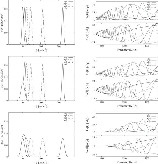
Absolute value of Faraday spectra of source models (left) and the corresponding polarized intensity without noise (right) for w1–w3 models of fiducial S/N source model from top to bottom.
A list of source models.
| Widtha σ1 = σ2 | σ1 = 0.5 | σ1 = σ2 | |
|---|---|---|---|
| = 0.25 | σ2 = 0.25 | = 0.5 | |
| Gapa ϕ2 − ϕ1 = 0.5 | w1g1 | w2g1 | w3g1 |
| 1 | w1g2 | w2g2 | w3g2 |
| 2 | w1g3 | w2g3 | w3g3 |
| 5 | w1g4 | w2g4 | w3g4 |
| 10 | w1g5 | w2g5 | w3g5 |
| Widtha σ1 = σ2 | σ1 = 0.5 | σ1 = σ2 | |
|---|---|---|---|
| = 0.25 | σ2 = 0.25 | = 0.5 | |
| Gapa ϕ2 − ϕ1 = 0.5 | w1g1 | w2g1 | w3g1 |
| 1 | w1g2 | w2g2 | w3g2 |
| 2 | w1g3 | w2g3 | w3g3 |
| 5 | w1g4 | w2g4 | w3g4 |
| 10 | w1g5 | w2g5 | w3g5 |
aIn units of the FWHM = 22.26 (rad m−2).
For equation (4) to calculate observable FDF, we select the frequency coverage from 700 to 1800 MHz (the FWHM 22.26 rad m−2) which is comparable to the early science program of Polarization Sky Survey of the Universe’s Magnetism (POSSUM) on Australian SKA Pathfinder (ASKAP). The channel width and the number are 1 MHz and 1100, respectively, so that the degree of freedom n is 2200 taking the Stokes parameters Q andU into account. Here it should be noted that, because we are discussing the source models in terms of the FWHM of RMSF, rather than the value of Faraday depth, most of the results obtained here are expected to be common with observations with other frequency range. Even though we choose a specific frequency coverage in our calculation, we can estimate the behaviour of general results at the different frequency coverage since our results are demonstrated in units of the FWHM of RMSF. Therefore, our simulation will be useful for upcoming observations such as with MeerKAT and the SKA. The Stokes Q and U spectra are shown in the right-hand panel of Fig. 1. To each channel of these synthesized spectra, we add random Gaussian white noise with the mean of 0 and the standard deviation of 1. Fig. 2 shows the Stokes Q and U spectra of w1g5 source model for three S/N cases, where the error bars indicate the input standard deviation. Integrated S/N for all of the mock data are summarized in Table 2. The source model of w3 is more depolarized than w1 model due to the large widths of Gaussian.
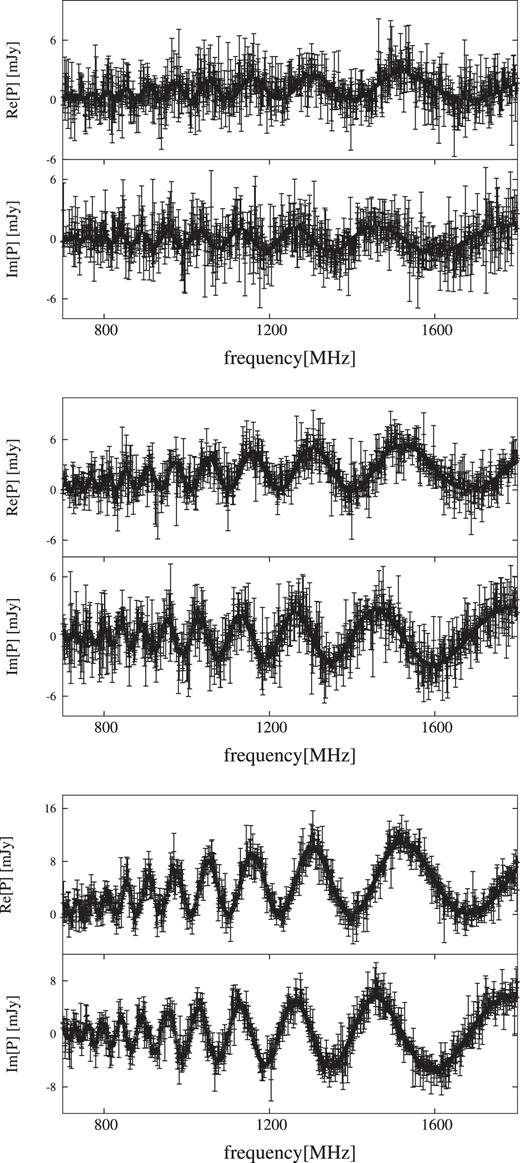
Simulation data including observational noise of w1g5 source model with three S/N models from top to bottom.
Integrated SNR for all of source models.
| |$f_1^a$| = f2 = 1.5 | f1 = f2 = 3 | f1 = f2 = 6 | |
|---|---|---|---|
| w1g1 | 53 | 68 | 109 |
| w1g2 | 58 | 82 | 142 |
| w1g3 | 74 | 124 | 235 |
| w1g4 | 67 | 107 | 198 |
| w1g5 | 69 | 112 | 208 |
| w2g1 | 54 | 70 | 114 |
| w2g2 | 53 | 69 | 111 |
| w2g3 | 67 | 107 | 199 |
| w2g4 | 62 | 93 | 167 |
| w2g5 | 63 | 97 | 177 |
| w3g1 | 50 | 59 | 85 |
| w3g2 | 49 | 53 | 69 |
| w3g3 | 60 | 89 | 157 |
| w3g4 | 56 | 76 | 127 |
| w3g5 | 57 | 80 | 138 |
aIn units of mJy.
We prepare four fitting models, G1, G2, G3, and G4, which consist of one to four Gaussian function(s), respectively. Because each Gaussian function has four parameters (see equation 10), the four models have 4, 8, 12, and 16 parameters, respectively. Physically, the four models have different numbers of polarized sources along the line of sight and, ideally, G2 model should be selected through the process described in the previous subsection.
Next, let us describe the MCMC method we use here. For given mock data and fitting model, we try to find the best-fittng parameter set using MCMC where parameter sampling is performed as follows (model parameters are denoted as a vector θ below).
Generate a candidate parameter set θ′ from the Gaussian distribution with the previous sample θt as average and the given step width as variance.
- Accept the candidate and update the parameter by setting θt + 1 = θ′ with the following probability uor otherwise the candidate is rejected by setting θt + 1 = θt. Here,(11)\begin{eqnarray*} u = \min \left(1,\frac{L(\theta ^{\prime })}{L(\theta _t)}\right), \end{eqnarray*}(12)\begin{eqnarray*} L(\theta) \propto \exp \left(-\frac{1}{2}\chi ^2(\theta)\right), \end{eqnarray*}where L(θ) is the likelihood given the parameter vector θ, χ2 is chi-square value, |$\lambda _i^2$| is the squared wavelength of i-th channel, |$P_{\rm obs}(\lambda _i^2)$| is mock data, |$P_{\rm mod}(\lambda _i^2;\theta)$| is the fitting model calculated with the parameter vector θ, σnoise is observational noise, and N is channel number. Note that the chi-square value becomes close to the degree of freedom n – 2200 when the model fits to the data well.(13)\begin{eqnarray*} \chi ^2(\theta) = \sum _{i=1}^N\left(\frac{P_{\rm obs}(\lambda _i^2)-P_{\rm mod}(\lambda _i^2;\theta)}{\sigma _{\rm noise}}\right)^2, \end{eqnarray*}
For each source model, we perform QU-fitting of four fitting models to the mock data 100 times with different random noise realizations. Thus, we perform QU-fitting, in total, (45 source models) × (4 fitting models) × (100 realizations) = 18 000 times.
3 RESULTS
Figs 3–5 summarizes the results of QU-fitting for the 45 source models. In each panel, the goodness of QU-fitting of 100 realizations are shown from the top to bottom. Each row has 18 coloured boxes and represents one realization. Colour indicates our criteria of goodness of QU-fitting described as follows:
Criterion (i): Four boxes from left to right in area (i) show the convergence of MCMC chain with the G1 to the G4 fitting models. Green means that all of the model-parameter searches are converged (satisfying Geweke’s diagnostics), and red is otherwise. Note that in red cases, MCMC is quit as reaching the maximum regulation number (100 000).
Criterion (ii): Four boxes from left to right in area (ii) show the chi-squared values for the G1 to the G4 fitting models, respectively. Green, yellow, orange, and red mean that the chi-squared value is smaller than 2231 (within 1σ of chi-squared distribution with n = 2200 degrees of freedom), 2231–2313 (2σ), 2313–2389 (3σ), and 2389 (out of 3σ), respectively. We regard the chi-square values as small (large) when it is smaller (larger) than 2389.
Criterion (iii): Left and right boxes in area (iii) show the model selection by AIC and BIC, respectively. Blue, green, yellow, and red mean that the G1, G2, G3, and the G4 fitting model was selected by the information criteria, respectively. Note that the source model always consists of two Gaussians and, therefore, the model selection is successful when the box is green.
Criterion (iv): Eight boxes from left to right in area (iv) show the accuracy of parameter estimation for the G2 fitting model (ϕ1, f1, χ0, 1, σ1, ϕ2, f2, χ0, 2, and σ2). Green, yellow, and orange mean the correct values are within 1σ, 2σ, and 3σ confidence regions, respectively, while red means the correct values are out of 3σ confidence region and parameter estimation is not successful. Note that this criterion is independent of criterion (iii), that is, the G2 fitting model is not necessarily selected by the information criteria.
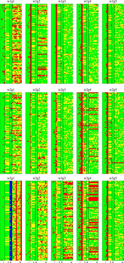
QU-fitting results for 15 source models of low-S/N case (see Table 1). The results for 100 realization simulations are shown. Colours are based on our criteria of quality assessment. Criterion (i): MCMC for the G1, G2, G3, and the G4 fitting models are converged (green) or not (red). Criterion (ii): the chi-squared values with the G1, G2, G3, and the G4 fitting models are located within 1σ (green), 2σ (yellow), 3σ (orange), or beyond (red) of the chi-squared distribution. Criterion (iii): AIC/BIC selected G1 (blue), G2 (green), G3 (yellow), or G4 (red). Criterion (iv): the estimated parameters of the G2 model are located in 1σ (green), 2σ (yellow), 3σ (orange), or beyond (red) of the probability distribution.
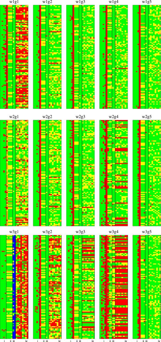
Same as Fig. 3 of fiducial S/N source models.
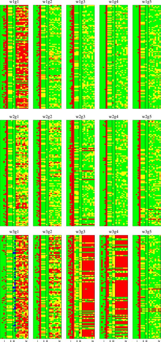
Same as Fig. 3 of high-S/N source models.
Generally, panels filled with many green boxes display that QU-fitting is effective. The effective cases tend to appear if a sum of the source widths is less than 1 FWHM (w2 and w1) and the separation of two sources is larger than 1 FWHM (g2–g5). We find a super resolution in some cases; two sources are resolved even if the separation is smaller than 1 FWHM. Meanwhile, QU-fitting often fails in some specific situations (section 4.1), although the separation is 5 FWHM or larger. As the SNR becomes higher, the ratio of finding a global maximum likelihood gets worse due to the difficulty of the model fitting.
Let us see the results more quantitatively. We count the success rates for the G2 fitting model on each criterion (i) convergence of MCMC chain, (ii) the chi-squared value within 3σ of the chi-squared distribution, (iii) selection by AIC/BIC, and (iv) all of eight true parameters are within 3σ of their L(θ). We regard the red boxes as the failure cases of QU-fitting, and the otherwise as the success cases. It should be noted that the above success rates are counted irrespective of the selected model. Fig. 6 shows the heat map of success rates in 100 realizations for all of S/N source models.
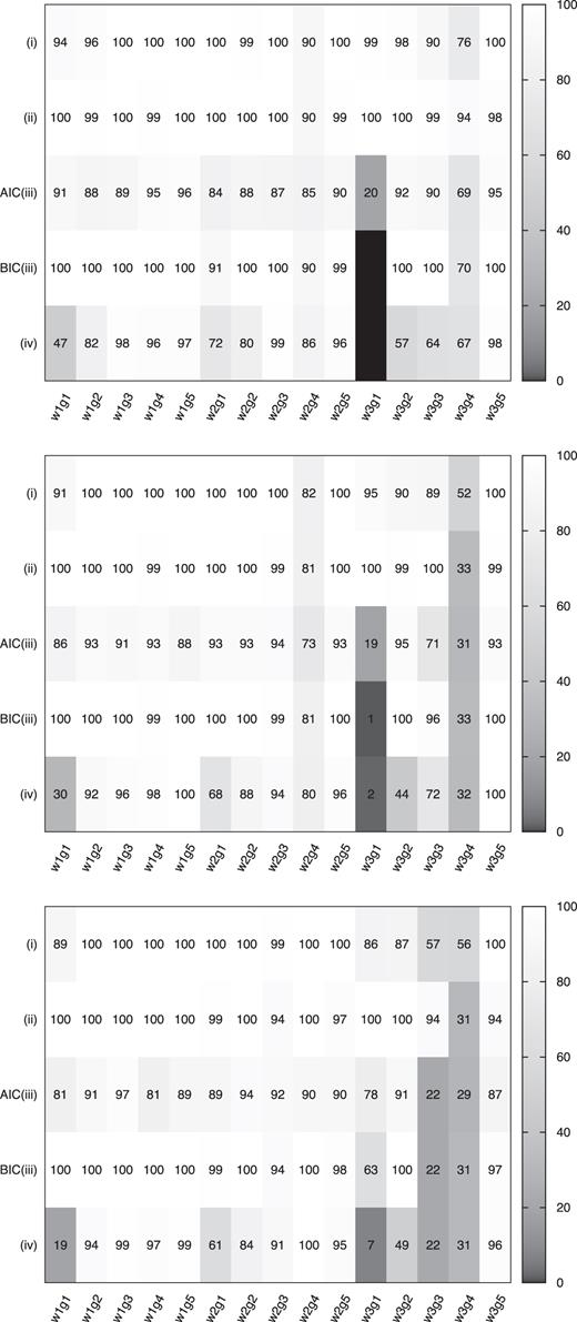
Heat map of success ratio (per cent) of QU-fitting by G2 fitting model for low, fiducial, and high-S/N source models from top to bottom panel, respectively. The number is the success ratio of 100 realization simulations for the individual Criteria (i)–(iv). We divide Criterion (iii) into AIC and BIC.
Moreover, in order to clarify at which step the QU-fitting fails to reproduce the source model, we define a categorization of the results as follows:
Class (A): The perfect case when all of the four criteria are satisfied the success line.
Class (B): Only a failure of parameter estimation, when Criteria (i)–(ii) are satisfied and Criterion (iv) is not satisfied the success line.
Class (C): Failure of parameter estimation and model selection, when Criteria (i)–(ii) are satisfied and Criteria (iii)–(iv) are not satisfied the success line.
Class (D): Failure of parameter estimation, model selection, and fitting to mock data, when Criterion (i) is satisfied and Criteria (ii)–(iv) are not satisfied the success line.
Class (E): The worst case when all of the four criteria are not satisfied the success line.
Here we note that Criterion (iv) is considered not to be satisfied when the correct parameter value is outside 3σ confidence region (red) for at least one of the eight parameters. When these four success lines are satisfied, we regard the results as the success cases of QU-fitting. We classify the rest cases as Class (Other), for example, Criteria (ii)–(iv) are satisfied the success line but Criterion (i) is not satisfied. We focus on these five classified results for the evaluation of QU-fitting since it is meaningless to consider the case when MCMC is not converged. Fig. 7 shows the percentages of the Classes (A)–(E) in 100 realizations for all of 45 source models. In the following subsections, we examine the results in Figs 6 and 7.
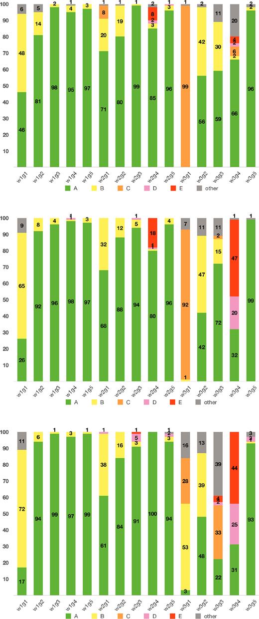
Results of the categorization Classes (A)–(E) for achievement of model fitting for low-, fiducial, and high-S/N source models from top to bottom panel, respectively.
3.1 Convergence of MCMC [Criterion (i)]
Fig. 6 shows that the convergence of MCMC is achieved and the success rate exceeds 80 per cent in all of source models except w3g3 and w3g4. The convergence rates of these two models are about 50 per cent because these two source models suffer from the situation that some of eight model parameters cannot reach the global maximum points in the parameter space. Overall, the score of the convergence of MCMC becomes worse as the S/N becomes higher (from top to bottom of Fig. 6), because the potential gradient of likelihood becomes steeper.
No strong correlation is found between MCMC convergence [Criterion (i)] and goodness of model parameter search [Criterion (iv)] as seen in Figs 3–5, because parameter estimation is not always good though MCMC chain is converged. On the other hand, Fig. 7 indicates that there are strong correlation between MCMC convergence and chi-squared value, that is, almost all of the source models are not categorized Class (D) except for w3g4 source. Convergence rate decreases as the number of model parameters increases from G1 to G4; however, it does not have simple correlation between the gap.
3.2 Chi-squared values [Criterion (ii)]
Fig. 6 shows that QU-fitting can find the fitting model which has a reasonable chi-squared value. Exceptions are seen in w3g4 and w2g4, both of which have the source separation of 5 FWHM. The success rate is only 30 per cent in w3g4, if the S/N is not low.
We obtain large chi-squared values with the G1 fitting model [the leftmost of Criterion (ii) in Fig. 3–5], indicating that two Gaussian sources cannot be fitted with a single Gaussian function. An exception is w3g1, whose two Gaussian components are so close in Faraday depth space that the source model looks like a single Gaussian (the solid line of the top-left panel in Fig. 1), In deed, w3g1 shows small chi-squared value with the G1 fitting model, regardless of the S/N. Generally, the model fit with larger number of model parameters produces smaller chi-squared value [see the G3 or G4 of Criterion (ii) in Fig. 3–5].
3.3 Model selection [Criterion (iii)]
Fig. 6 shows that AIC and BIC select the correct model (G2 fitting model) with the percentages of 70–90 per cent and 80–100 per cent, respectively, except for w3g1, w3g3, and w3g4 source models. For the w3g1 source, AIC (BIC) selects G1 as the best-fitting model at the rate of 70–80 per cent (99 per cent) in low-S/N case, however AIC (BIC) tends to select the G2 for 80 per cent (60 per cent) in high-S/N case. On the other hand, in the case of w2g1 and w1g1 sources, both AIC and BIC show high success ratio more than 80 per cent, although there are also actually two Gaussian sources overlapping each other having the same small gap. AIC and BIC tend to select G3 in high-S/N source model of w3g3 and w3g4 for 60–70 per cent (see Section 4.1 for further discussion).
Comparing AIC and BIC, BIC generally has slightly higher scores except w3g1 source. Because the sum of two Gaussian functions cannot be expressed as a single Gaussian, fitting w3g1 mock data with the G1 fitting model cannot be perfect. Nevertheless, because the penalty imposed by BIC is relatively large, it will tend to select the G1 model.
3.4 Parameter estimation [Criterion (iv)]
Quality of parameter estimation significantly depends on the source model. Overall, if the widths of two Gaussian sources are smaller than 0.5 FWHM and the separation of two Gaussian sources are larger than 1 FWHM, QU-fitting can estimate the parameters with good accuracy. Otherwise, failure of parameter estimation becomes appreciable, e.g. w3g1, w3g2, w3g3, w3g4, w2g1, and w1g1. The success rate of w3g1, w2g1, and w1g1 are 0–10, 60–70, and 20–40 per cent, respectively, in any S/N situations.
Finding two Gaussians for the case of large Gaussian widths is challenging, as seen in w3g1 which cannot be separated into two Gaussians. Even if the Faraday spectrum shows a double-peak profile, we get a poor estimation (w1g1). Nevertheless, QU-fitting tends to show a good reconstruction for w2g1 in which two Gaussians have different widths. We will take a close look at the reason of this phenomenon in Section 4.2.
The separation of two Gaussian sources is another key factor of the quality of parameter estimation. The success rate clearly depends on the separation; 50, 60–70, and >95 per cent for w3g2, w3g3/w3g4, and w3g5, respectively. Note that these low rates are caused by poor estimations of only a few of eight model parameters. The rate also depends on the S/N; it decreases to 20–30 per cent for w3g3/w3g4, for instance, at the high-S/N situation.
4 DISCUSSION
In this section, we investigate w3g4 source model which QU-fitting does not work well to clarify the tendencies of the results, and discuss the success case of w2g1 source. Overall, these models are the cases with relatively thick Faraday spectra and/or a relatively narrow gap between two components.
4.1 Failure with large gap model (w3g4 source)
Overall, QU-fitting can find the right solution, if a sum of the source widths is less than 1 FWHM and the separation of two sources is larger than 1 FWHM (section 3). However, although w3g4 source model satisfies this condition, very low scores for all of criteria (i)–(iv) are found; Fig. 7 shows that w3g4 is classified into the worst rank Class (E) about 50 per cent in fiducial or high-S/N models.
One of the reasons of this failure is that the chain is trapped in a local maximum of the likelihood function in parameter space. Fig. 8 shows the distribution of best-fitting Faraday depths of two sources in 100 realization simulations, where the colour indicates the chi-squared values of the fit. The global maximum likelihood is located at ϕ1 = 0 (rad m−2) and ϕ2 = 111.3 (rad m−2), around which 30 per cent of the simulations successfully reached. There is also a local maximum area at ϕ1 = 40–60 (rad m−2) and ϕ2 = 50–70 (rad m−2), and 70 per cent of the simulations are trapped there. The 20 out of 70 failure cases are categorized into Class (D). It means that the MCMC is converged into a local maximum spot in each parameter space. In the rest 50 cases, we find that the MCMC chain wanders in parameter space and is not converged. The results are categorized as Class (E).
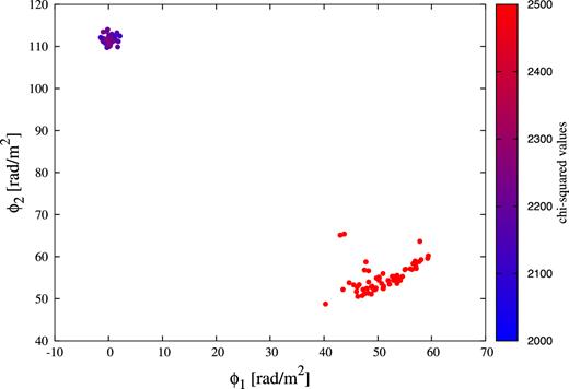
Correlation of estimated best-fitting Faraday depths of two sources in 100 realizations of w3g4 source. Colour indicates the chi-square values calculated by equation (13).
Because we set the initial values of all parameters to 0 as is often done, trapping in local maxima can often happen depending on the structure of the likelihood function. This case could be avoided, if we adopt reasonable initial values provided from other analyses such as RM CLEAN. Fig. 9 demonstrates RM CLEAN using simulation data of w3g4 source. RM CLEAN misestimates the source width and intrinsic polarization angle (because it cannot resolve a structure smaller than FWHM), but it can estimate the location of the two peaks in ϕ space correctly. RM CLEAN is known to show good performance when the gap between the two source is larger than 1FWHM (Kumazaki et al. 2014; Miyashita, Ideguchi & Takahashi 2016). Therefore, if the RM CLEAN reproduces the model which has double peaks and the gap is more than 1FWHM, it is better to set the value of the parameter calculated by RM CLEAN as the initial value of QU-fitting, then the performance of QU-fitting could be improved. This initial-guess issue is beyond the scope of this work and we will address it in a separate paper.
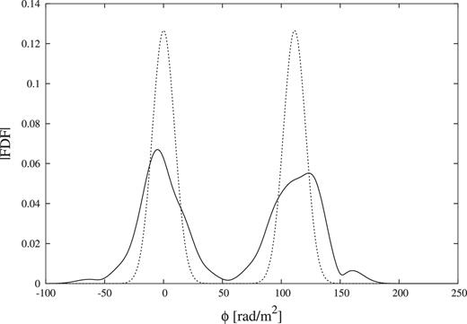
Cleaned FDF (solid line) constructed by RM CLEAN using simulation data of w3g4 source, which is same one of QU-fitting test simulation and the source model FDF (dotted line) of w3g4.
QU-fitting sometimes overestimates the number of components. In particular, for w3g4, BIC selected G3 and G4 fitting model 51 and 16 times out of 100 realizations, respectively. All of the 67 cases are categorized as the worst case Class (E) (see Fig. 7), where fitting with the G2 model failed completely (like Fig. 8). Thus, when the G2 model fails to fit, the G3 model tends to be selected. When fitting is performed with G3 model, it often happens that two of the components reproduce the true components correctly, while the last one is located at large absolute Faraday depth with a large thickness. Fig. 10 shows the reconstructed Faraday spectra of 15 examples out of the 51 realizations which select the G3 fitting model for w3g4. As we can see, there is a Faraday-thick component at large absolute Faraday depth. In fact, the extra component does not significantly contribute to polarized intensity in the frequency range of ASKAP because of strong depolarization effect. Therefore, we expect that such an extra component with a width larger than the max-scale (the largest scale in ϕ space to which one is sensitive) can be recognized as a fake, and then removed.
![Reconstructed Faraday spectra with G3 fitting models for w3g4. The top left panel shows the w3g4 source model [ϕ1 = 0 (rad m−2), ϕ2 = 111.3 (rad m−2)].](https://oup.silverchair-cdn.com/oup/backfile/Content_public/Journal/mnras/482/2/10.1093_mnras_sty2862/1/m_sty2862fig10.jpeg?Expires=1749936801&Signature=imSX8pnaQkkOxbU9IXp3i0rejGm9TzS1sYSJhrW6X8--FK4owJ3gX8Vz-DiQNdOtLotfA~FHXpiYHPLAGRqb~Th5eaeKRmIyqGo-~Ey4F67yyEclQN6WvjSLaXGzV-WPXK6kME-BS4nRl-bKd7sTKJAkFt~Lu93ZN584tEivshNmjT~PyRZPbhvFsq4~qAuQUVy45tpJTOWrQxmt9rqOgZ6fxBDIjl3ykifoCT8xcIisIjVc07WL1xgN7Ovbkbkx72Blc-KEpx0Lj94HvW4DiImzzuWML7qjTtpNicjSINoluL7DzMUdDYslpjFHpwpu3ZdGEam0tMJAKYrT4QD8Sg__&Key-Pair-Id=APKAIE5G5CRDK6RD3PGA)
Reconstructed Faraday spectra with G3 fitting models for w3g4. The top left panel shows the w3g4 source model [ϕ1 = 0 (rad m−2), ϕ2 = 111.3 (rad m−2)].
Another possible reason of the failure seen in w3g4 is the dependence of intrinsic polarization angle, as discussed in previous works (Kumazaki et al. 2014; Miyashita et al. 2016). In order to examine this effect, we perform our simulations again by changing only the intrinsic polarization angle of one of the two Gaussians for w3g4 source into χ0, 2 = |$\pi$|/2 or |$\pi$|/3. Fig. 11 shows the categorization results same as Fig. 7 of w3g4 with different intrinsic polarization angles. We can see that the results strongly depend on the intrinsic polarization angle difference. QU-fitting shows high scores; 90 realizations are categorized into the best case Class(A) in the case of Δχ0 = |$\pi$|/3. Therefore, the location of the local maximum can be varied by the model parameters.
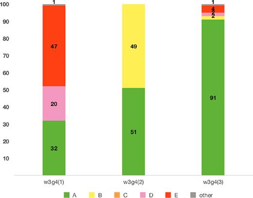
Results of the categorization Classes (A)–(E) for achievement of model fitting (same as Fig. 7) for w3g4 source with different intrinsic polarization angle of second Gaussian. Individual cumulative bar chart shows the result of fiducial χ0, 2 = |$\pi$|/4 (rad) labelled as w3g4(1), χ0, 2 = |$\pi$|/2 labelled as w3g4(2), and χ0, 2 = |$\pi$|/3 labelled as w3g4(3), from left to right, respectively.
4.2 Unresolved models (w3g1/w2g1/w1g1 sources)
The source models of w3g1, w2g1, and w1g1 consist of two Gaussian sources whose separation in Faraday depth is a half of the FWHM of RMSF. Differences among the models are the widths of Gaussians, which alter apparent shape of Faraday spectrum from single peak (w3g1), asymmetric (w2g1), to double peaks (w1g1). As shown in Section 3.4, this difference impacts on the performance of QU-fitting; w3g1, w2g1, and w1g1 sources are categorized into Class (C; 90 per cent), Class (A; 70 per cent), and Class (B; 70 per cent), respectively (see Fig. 7). Interestingly, these scores do not simply depend on the amount of the Gaussian widths.
For a single peak FDF (w3g1), both AIC and BIC tend to make erroneous model selection. Fig. 12 shows the distribution of estimated best-fitting Faraday depths of w3g1 source in 100 realizations. It indicates that the second component is located at large absolute Faraday depth with a large source width. A similar phenomenon is already seen in Fig. 10; this component is strongly self-depolarized and does not significantly contribute to the polarized-intensity spectrum. Thus, AIC/BIC chooses the G1 rather than G2 fitting model.
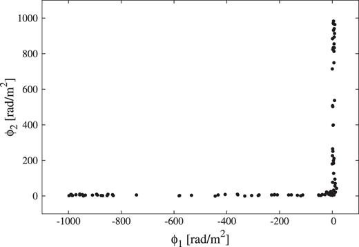
Correlation of estimated best-fitting Faraday depths of two sources for w3g1 source in 100 realizations.
Essentially, it is hard for us to recover (resolve) the FDF with multiple components within a FWHM resolution. Indeed, MCMC failed to fit two sources in w1g1, even though the model has a double-peak profile. However QU-fitting represents high scores in w2g1, although two Gaussians overlap each other. We suspect that a different amount of depolarization caused by the different Gaussian widths is a key to identify these unresolved components.
Depolarization is mostly determined by the Gaussian width, but sources with different amplitudes also indicate a different amount of depolarization mathematically in frequency space. In order to examine the latter depolarization, we perform our simulation again and change the amplitudes of w3g1 source, f1 = 2, f2 = 4 (mJy) (same S/N as fiducial S/N model), keeping the Gaussian widths. Fig. 13 shows the modified model FDF of w3g1. The FDF has a very small skewness due to the small gap. Table 3 shows a comparison of the categorization results using Classes (A)–(E) between two cases of w3g1 source which has same/different Gaussian amplitudes. It shows that the results almost never changed; both AIC and BIC fail model selection about 90 per cent rates because we cannot see the difference between G1 and G2 spectra in the ASKAP bands. We conclude that source width is more effective for the performance than source amplitudes.
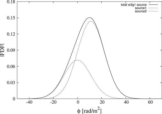
Absolute value of model FDF of w3g1 source only changed the amplitudes of f1 = 2, f2 = 4 (mJy) (solid line) and each Gaussian components (dotted line).
| (A) | (B) | (C) | (D) | (E) | Others | |
|---|---|---|---|---|---|---|
| w3g1 | 0 | 1 | 92 | 0 | 0 | 7 |
| w3g1 + | 0 | 2 | 88 | 0 | 1 | 9 |
| (A) | (B) | (C) | (D) | (E) | Others | |
|---|---|---|---|---|---|---|
| w3g1 | 0 | 1 | 92 | 0 | 0 | 7 |
| w3g1 + | 0 | 2 | 88 | 0 | 1 | 9 |
| (A) | (B) | (C) | (D) | (E) | Others | |
|---|---|---|---|---|---|---|
| w3g1 | 0 | 1 | 92 | 0 | 0 | 7 |
| w3g1 + | 0 | 2 | 88 | 0 | 1 | 9 |
| (A) | (B) | (C) | (D) | (E) | Others | |
|---|---|---|---|---|---|---|
| w3g1 | 0 | 1 | 92 | 0 | 0 | 7 |
| w3g1 + | 0 | 2 | 88 | 0 | 1 | 9 |
Finally, we discuss the appearance of RM ambiguity (Farnsworth, Rudnick & Brown 2011; Kumazaki et al. 2014; Miyashita et al. 2016; Brown et al. 2018). In the situation of w3g2 source model, the gap of two sources Δϕ is 1FWHM and the difference of intrinsic polarization angle Δχ0 is −45 (deg), Kumazaki et al. (2014) reported the false signal appeared between two sources. In other words, RM CLEAN cannot reconstruct the FDF correctly in this situation. However, Fig. 7 shows the QU-fitting successes to reproduce the correct FDF model for 50 per cent, and Fig. 14 shows the reconstructed FDF using RM CLEAN and QU-fitting. The rest 50 per cent case is classified into Class (B), so QU-fitting can separate two sources with no false signals.
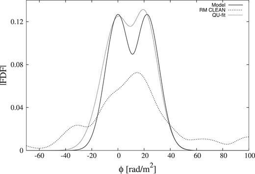
Calculated cleaned FDF by RM CLEAN and reconstructed FDF by QU-fitting of w3g2 model.
5 SUMMARY
In this paper, we examined the functionality of standard QU-fitting algorithm quantitatively by simulating spectro-polarimetric observations of two extent sources located along the same LOS. We assumed the Gaussian function as a model of the extent sources and varied the gap, width and S/N of the two Gaussians systematically. Especially, focusing on the convergence of MCMC chain, obtained chi-squared value, model selection by AIC and BIC, and parameter estimation, we evaluated the effectiveness of QU-fitting. For source models with a gap between two sources is larger than 1 FWHM, QU-fitting works well. Contrastingly, overlapping thick sources are difficult to be separated (w3g1), while overlapping thin sources can be separated (w2g1 and w1g1). Further, even if two sources do not overlap with each other, model selection and/or parameter estimation often fail for sources as thick as the FWHM determined by the observation frequency band (w3g2, w3g3, and w3g4). This is partly due to the trapping of MCMC chain to a local maximum of likelihood function. Thus, it is implied that we need more advanced techniques to study such simple sources as two Gaussians with QU-fitting. As the S/N becomes higher, the ratio of finding a global maximum likelihood gets worse because of the difficulty of the model fitting. If we could obtain rough estimate of parameter values from RM CLEAN, for example, QU-fitting works even better by setting the initial values of MCMC chain to the estimated values. We considered these four criteria of the quality of QU-fitting independently.
However, in fact, they are closely related to each other. For example, if the obtained chi-squared value is large even though the MCMC chain is converged, it is interpreted that the chain was trapped in a local maximum of likelihood function. In this case, model selection and parameter estimation would also fail. To avoid this type of failure, more sophisticated algorithm of MCMC will be necessary. Another possible example is a case where the MCMC chain is converged and a reasonable chi-squared value is obtained, but model selection is failed. This example would imply the limitation of the information criterion.
In the era of large polarization surveys such as POSSUM and SKA, data for millions of sources will be processed with automatic pipelines. Our simulations of dozens of models foresee potential problems of the pipelines. Abort of MCMC and miss-fitting with a large chi-squared values are likely, but they are rather acceptable failures because the pipelines can recognize the failures and can flag out the source to take a close look at it later. A more serious problem is the case that the pipelines cannot find any signature of failure. Our study highlighted the specific case in which QU-fitting suggests that one of the multiple component is located at very large Faraday depth with a large Gaussian width. The pipelines should incorporate e.g. Burns law (Burn 1966) and must identify this artefact; a clue is that such a component is significant in Faraday spectrum but is not contributing to the polarized intensity due to self-depolarization.
ACKNOWLEDGEMENTS
This work is supported in part by Grand-in-Aid from the Ministry of Education, Culture, Sports, and Science and Technology (MEXT) of Japan, No. 17J06936 (YM), 24340048 (KT), 26610048 (KT), 15H03639 (TA), 15H05896 (KT), 15K17614 (TA), 16H05999 (KT), and 17H01110 (TA, KT), Bilateral Joint Research Projects of JSPS (KT).
