


Abstract
Atmospheric turbulence limits the angular resolution of ground-based optical telescopes. The daytime turbulence conditions for solar observations are stronger and more complicated than the turbulence observed at night. The Baikal Astrophysical Observatory is the site of the 1-m Large Solar Vacuum Telescope (LSVT) located near Lake Baikal (East Siberia, Russia), which is the largest freshwater lake in the world. The region hosts unique weather regimes and natural phenomena, including local winds and giant ice rings. Because the LSVT has ongoing and planned programmes in adaptive optics (AO), statistical knowledge of atmospheric turbulence and wind speed distributions is essential for designing and optimizing AO systems. We present the first seasonal study of the vertical distribution of wind speed and daytime optical turbulence conditions at the Baikal Astrophysical Observatory. Site measurements of the daytime Fried parameter were collected using the Shack–Hartmann wavefront sensor in the LSVT AO system. Reanalysis data from the National Centers for Environmental Prediction (NCEP) and the National Centers for Atmospheric Research (NCAR) were used to characterize the wind speed distribution. The results demonstrate seasonal variation in both solar seeing and wind speed profile. The strongest wind speed was detected in winter and in November, while the weakest wind speed occurred during summer. The strongest daytime turbulence conditions were observed in the winter. The best solar seeing β0 ≈ 1 arcsec was detected in the summer.
1 INTRODUCTION
The Baikal Astrophysical Observatory (BAO; latitude 51°50′ north, longitude 104°55′ east) of the Institute of Solar-Terrestrial Physics, Siberian Branch of the Russian Academy Sciences, is located at an elevation of approximately 700 m above sea level on the shore of Lake Baikal in East Siberia, Russia. The Large Solar Vacuum Telescope (LSVT) is the main telescope of the BAO. The LSVT 1-m off-axis primary mirror is mounted on a vertical column 25 m high. The vacuum tube is inclined at an angle of 52° to the horizon (Fig. 1). This allows spectropolarimetric observations of the Sun in both infrared and visible spectral ranges.
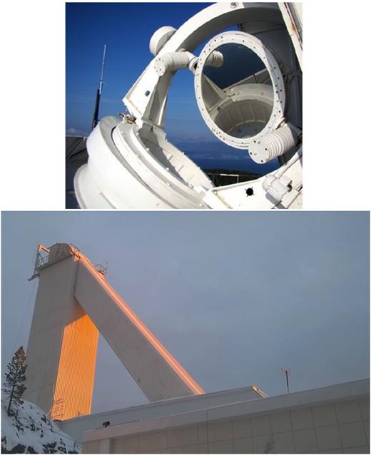
The LSVT of the BAO.
The telescope is equipped with a first-generation Angara adaptive optics (AO) system, developed by the Institute of Atmospheric Optics, Siberian Branch of the Russian Academy Sciences. There are ongoing and planned programmes in AO for the LSVT (Antoshkin et al. 2017).
Daytime turbulence conditions are stronger than optical turbulence at night, although measurements for solar telescopes are sparse. Detailed studies of solar seeing have been conducted at numerous locations globally, including the Big Bear Solar Observatory (BBSO) in California, the Mees Solar Observatory (MSO) on Haleakala, Maui, Hawaii, and the Observatorio Roque de los Muchachos on La Palma, Spain. Additional work has been completed during surveys to identify sites for the 4-m aperture Advanced Technology Solar Telescope (ATST; Socas-Navarro et al. 2005; Verdoni and Denker 2007) and the Indian National Large Solar Telescope (Dhananjay 2014). Daytime turbulence measurements were made above La Palma (Scharmer and Van Werkhoven 2010), Big Bear Lake (Kellerer et al. 2012), Antarctica (Okita et al. 2013) and at the Teide Observatory on Tenerife, Canary Islands (Sprung et al. 2016). Several methods have also been developed in order to accurately measure solar seeing (Beckers 2001; Scharmer and Van Werkhoven 2010; Ikhlef et al. 2016).
The wind speed at the 200-mbar pressure level (V200) has been proposed as a parameter for estimating the suitability of an astronomical site for AO capabilities (Sarazin and Tokovinin 2002), which is supported by empirical results from Chilean sites. Initially, a similar seasonal trend between seeing and V200 was found by Vernin (1986) at La Silla and Mauna Kea. Subsequently, V200 was studied at several astronomical sites (Carrasco, Avila & Carramin 2005; Socas-Navarro et al. 2005; García-Lorenzo et al. 2009). Without additional data, it is clear that V200 alone is insufficient to comprehensively prepare for AO, and vertical wind speed profiles are necessary (García-Lorenzo et al. 2009; Masciadri et al. 2010). The simplest method to characterize vertical distributions of wind speed is to use reanalysis data. The vertical distribution of wind speed has been studied at several astronomical sites, including at some sites the use of estimates produced from National Centers for Environmental Prediction (NCEP)/National Centers for Atmospheric Research (NCAR) reanalysis data (Chueca et al. 2004; García-Lorenzo et al. 2005; Hagelin, Masciadri & Lascaux 2010; Hach et al. 2012; Sanchez et al. 2012).
No previous study has investigated the vertical distribution of wind speed and V200 at the BAO site. Early work on characterizing optical turbulence at the BAO was conducted using a Brandt sensor (see Brandt 1969 for details of this method). Ground turbulence conditions were analysed with sonic anemometers placed near the telescope, and coherent structures in the surface layer were detected in the summer under various meteorological conditions (Lukin et al. 2016). However, solar seeing measurements over different seasons at the BAO had not been performed, until now.
We present the first seasonal study of the vertical distribution of wind speed and daytime atmospheric optical turbulence conditions at BAO near Lake Baikal.
The paper is organized as follows. In Section 2, we introduce some of the geographical and climatological features that make the BAO a unique site for solar observation. In Section 3, we present an analysis of the vertical distribution of wind speed conditions above the BAO from NCEP/NCAR reanalysis data. In Section 4, we describe the instrument and data analysis of the Fried parameter for daytime atmospheric turbulence.
2 LOCAL CLIMATE AND ITS IMPACT ON OBSERVATIONS
Lake Baikal covers an area of 31 570 km2 in East Siberia, and is the deepest freshwater lake in the world (Galaziy 1988). The volume of water in Lake Baikal is about 23 000 km3, making it the world’s most voluminous freshwater lake. The lake has experienced unprecedented warming over the most recent decades. It is covered with ice for almost 4.5 months annually. The water temperature in the surface layer changes from +15° C in August to 0° C in December and January. On average, the freezing of Lake Baikal begins on December 21, and ends between January 8 and 16, but it takes about a month to completely freeze. The ice breaking begins around April 25–30, where the average date of full opening is May 4–6. Lake Baikal influences the local coastal climate, and this includes the climate at the BAO site.
The continental climate of Siberia, characterized by long cold winters and short hot summers, also influences the shore of Lake Baikal. However, the average temperature in December on the shores of Lake Baikal is 13–15° C higher than locations distant from the lake. In summer, temperatures on the banks are lower by 7–10° C. The large volume of the lake smooths temperature fluctuations, with summer maintaining cooler temperatures and winter consistently warmer than in neighbouring regions. The hottest month is August. Water, heated over the summer, continues to provide residual heat to the surrounding area in autumn, so September is also warm. Furthermore, the onset of spring at Lake Baikal is delayed by 10–15 d compared with adjacent areas.
Local climate is greatly influenced by the surrounding mountains, as well as cold water, which is slowly heated. Typical of such sites, the cool water of the lake does not allow the heating of the ground surface, which improves solar observations in summer. The lake determines the distribution of solar radiation and air temperature. More than 60 per cent of the solar radiation is absorbed by the upper water layer of Lake Baikal, and more than 80 per cent is absorbed by the upper 10 m. The effect depends on the zenith angle, and is at its maximum at noon. Therefore, we expect an improvement in the solar seeing at this time. In winter, when the lake is covered with ice, the lake ice albedo varies greatly depending on ice type (e.g. white, snow and blue ice), bubble content, ice thickness and the presence of impurities. Furthermore, Lake Baikal has several unique hydrological and weather regimes and other natural phenomena, including local winds and giant ice rings (Ivanov 2012). However, the influence of these effects on solar observations has not yet been studied.
The lake is characterized by the absence of cloud cover. In spring and summer, evaporation is insignificant from the cool water surface, and clouds cannot form. Airmasses bring clouds from the land surfaces to Baikal, when the surrounding mountains are heated, but the clouds are scattered. This characteristic provides good conditions for satellite images; in images, the sky over the lake is cloudless, and the areas at the lake shore are covered with thick clouds. The maximum atmospheric transparency of air occurs in the autumn–winter period, and the minimum occurs in spring–summer.
The first historical reports of seeing conditions at Lake Baikal were made by Kovadlo, Ivanov & Darchia (1972), who noted the stabilizing effect of a large water area and the local climate.
3 WIND SPEED DISTRIBUTIONS
The simplest method of characterizing the vertical distributions of wind speed is to use NCEP/NCAR reanalysis data. The data set was created through the cooperative efforts of the NCEP and NCAR to produce relatively high-resolution global analyses of atmospheric fields over a long time period (Kistler et al. 2001). This data set is constrained by the availability of observations, such as land, marine, balloon, satellite and aircraft data, and includes U and V components of the wind speed every 6 h at 17 different pressure levels. Research has shown that NCEP/NCAR reanalysis wind data are robust and suitable for characterizing astronomical observatories (Avila et al. 2006; Hach et al. 2012). We analysed NCEP/NCAR reanalysis wind speed data from 1948 to 2016 at the BAO site in order to characterize wind speed in terms of monthly vertical distribution and seasonal behaviour.
NCEP/NCAR reanalysis data were obtained for four grid points close to the observatory: 50°0′ N, 102°5′ E; 50°0′ N, 105°0′ E; 52°5′ N, 102°5′ E; 52°5′ N, 105°0′ E. Following the work of Chueca et al. (2004), we compared wind speed statistics from the NCEP/NCAR reanalysis data with direct measurements using radiosonde balloon flights from Irkutsk (latitude 52°27′ N, longitude 104°35′ E), which is close to the observatory. The Irkutsk station is part of the Federal Service for Hydrometeorology and Environmental Monitoring of Russia (Roshydromet) network. Radiosondes are launched twice daily. We obtained good correlations between NCEP/NCAR reanalysis data and radiosonde balloon data for mean monthly values (Fig. 2).
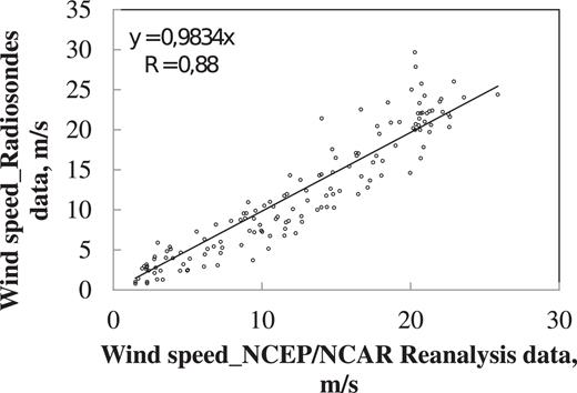
Comparison of the NCEP/NCAR reanalysis and radiosonde balloon data for mean monthly values of wind speed.
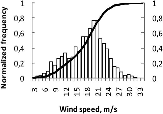
Fig. 3 shows the frequency and cumulative distribution of the wind speed from NCEP/NCAR reanalysis data corresponding to the period 1948–2016.
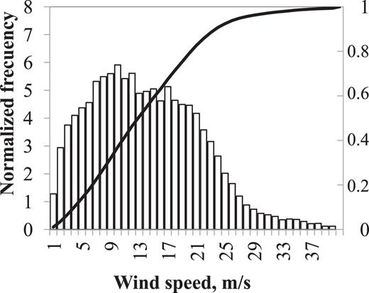
Histogram and cumulative distribution of the wind speed from the NCEP/NCAR reanalysis data corresponding to the period 1948–2016.
We have split all available seasonal data for wind speed corresponding to each month from the NCEP/NCAR reanalysis data and we have calculated the median wind speed and the first (25th) and third (75th) quartiles (Fig. 4).
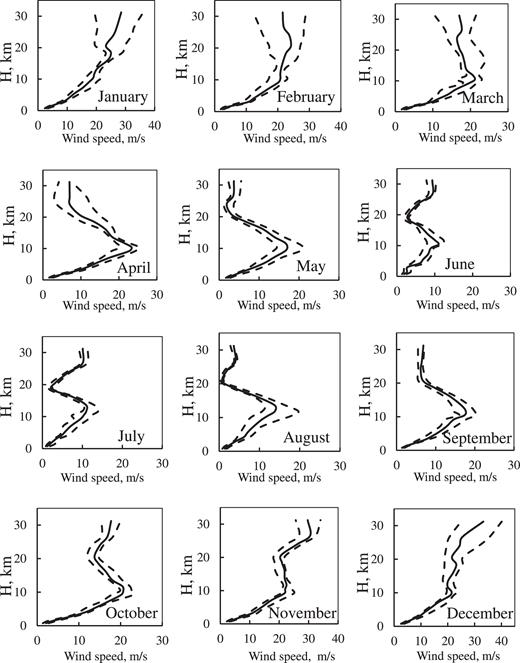
Median wind speed profiles calculated from the NCEP/NCAR reanalysis data for each month during 1948–2016 (solid line). The dashed lines represent the first and third quartiles.
Fig. 5 shows the average of the vertical profiles of wind speed for 1996–2016 at the 925 to 10 mbar atmospheric pressure levels. The monthly wind speed results at the BAO site over the same period are presented in Table A1 in the Appendix.
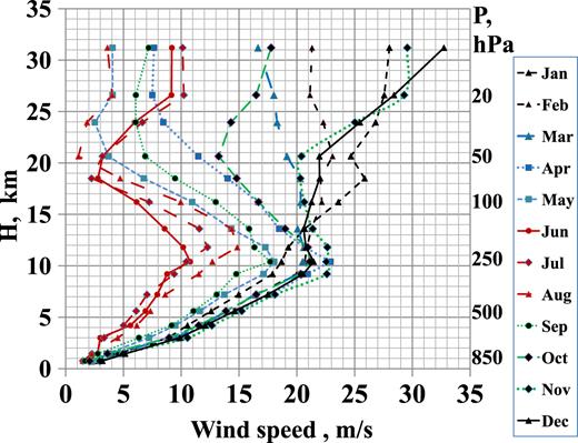
Monthly averages of vertical wind speed profiles from the NCEP/NCAR reanalysis data corresponding to the period 1996–2016.
Large differences in vertical wind behaviour are observed between summer and winter. November has the strongest wind speed, while the weakest wind speed is observed in June and July. There are also significant differences in seasonal conditions with several types distinguishable.
Wind vertical distributions show paired similarity in April and October, May and September, and November–March, matching the similar weather conditions in Siberia. May–September constitutes the warm season at the BAO site. The January data are unique to the data set, although the most interesting aspect of this plot is the wind speed behaviour from December to February. Above 180 mbar (an altitude of 12 km above sea level) during winter, wind speed increases rapidly with altitude and reaches a maximum that does not appear in other seasons. Excluding the winter season, wind speed profiles show a maximum at the jet-stream level (200 mbar).
Seasonal variations in wind speed profiles are easily identified in Fig. 5, particularly in the winter and summer periods. The wind speed profiles are different, with the strongest high-altitude wind speed during winter and November. The interquartile range shows the differences between the individual years, with the greatest differences during the winter – in November, March and April – for high-altitude wind. Smaller differences between the first and third quartiles are observed in the summer – in May, September and October – except for the jet-stream level and particularly for August. This result indicates year-to-year variability of wind speed in the jet stream.
We further analysed wind speeds at the 200-mbar level for 1948–2016 from the NCEP/NCAR reanalysis data.
Fig. 6 shows the frequency and cumulative distribution of the V200 wind speed. The wind speed distribution has a bimodal shape, where the low wind speed distribution has a mean of 12 m s–1 and high wind speeds are at 20 m s–1. This might indicate two different wind speed regimes: a summer regime and another at all other times. Furthermore, the two different distributions could be a signature of seasonal variations in the Fried parameter.
Histograms and cumulative distribution of V200 from the NCEP/NCAR reanalysis data for the period 1948–2016.
The V200 seasonal behaviour is plotted in Fig. 7 as monthly averages. Table A2 shows the statistics derived for each month, including the standard deviation of the annual average values (std), mean and median values.
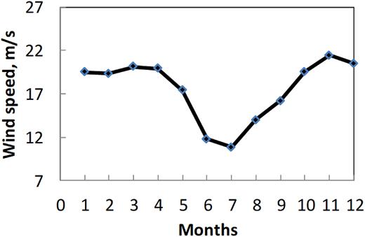
Monthly average 200-mbar wind speed from the NCEP/NCAR reanalysis data for the period 1948–2016.
The tropopause data from the NCEP/NCAR reanalysis confirm the seasonal evolution of the tropopause layer (Fig. 8). The tropopause is higher in summer than in winter. Both the tropopause and jet stream demonstrate seasonal variation above the BAO.
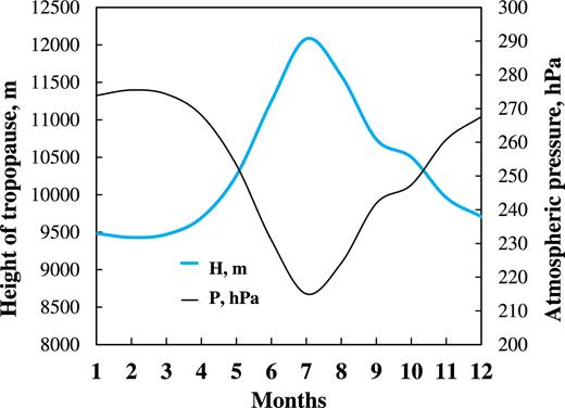
Height of tropopause above the BAO from NCEP/NCAR reanalysis data.
4 DAYTIME FRIED PARAMETER
The measurements of coherence length, or Fried parameter, were collected at the BAO site with a Shack–Hartman wavefront sensor (S–H WFS) installed on the LVST AO system, as described by Antoshkin et al. (2017). Using part of a solar AO system to measure seeing has been previously discussed by Kawate et al. (2011) and Kellerer et al. (2012). Each pair of subapertures is regarded as a differential image motion monitor (DIMM), where seeing is estimated from differential image motion (Sarazin and Roddier 1990). Differential motions of the limb of the Sun have been observed with the solar DIMM in order to calculate the daytime Fried parameter (Beckers 2001; Ozisik and Ak 2004). Sunspots can serve as good targets for a DIMM, but their size, shape and presence on the disc change from day to day (Kawate et al. 2011).
In our research, the regions of the solar image with contrasting elements (sunspots or solar granulations) were detected using the CCD camera of the S–H WFS by attaching the solar filter (λ = 535 nm), and centroid coordinates were computed using the correlation algorithm (Lukin et al. 2010).
The transverse and the longitudinal components of the displacement are accounted for using the calculated mean r0 (transv + longit)/2.
First, we used the CCD camera Prosilica GE-680 with a resolution of 640 × 480 pixels, as detailed in Lukin et al. (2010). Then, we improved this methodology with the design of the S–H WFS, which incorporated the CCD camera Prosilica GX-1050 with a resolution of 1024 × 1024 pixels (Botygina et al. 2018). The pixel sizes are 7.4 and 5.5 μm for GE-680 and GX-1050, respectively. We used lenslet arrays containing a number of subapertures with 8 × 8. The size of subaperture relative to the LSVT entrance pupil is 67.08 mm. The angular scale of the CCD pixel transforms the measured centroid variance from pixels to radians. We cannot rely on the nominal pixel scale because all individual telescopes are slightly different and the scale depends on various factors (Kornilov et al. 2007). The pixel scales in the angular unit relative to the LSVT telescope focal plane are 0.83 and 0.55 arcsec, respectively.
The exposure time of the detector is another crucial parameter for seeing studies using the DIMM. It is necessary to use the shortest exposure time allowed by the hardware and noise (Tokovinin 2002). We used the exposure time of 1 ms.
It has been pointed out by Sarazin and Roddier (1990) that the statistical properties of the atmosphere only change after about a minute. So, for longer time-scales, the value of r0 will change substantially, as the seeing conditions evolve. In our study, the accumulation times were 42 s (GE-680) and 43 s (GX-1050). The differential variance of the wavefront tilt is estimated from the finite number of frames N. To measure the seeing with a relative error of 2 per cent, N must be greater than 1800. With a 1-min accumulation time, a frame rate of 30 Hz or larger is required. In fact, the statistical error of seeing measurements will be larger because frames are partially correlated and are non-stationary (Kornilov et al. 2007). For this study, we used the acquisition rates of 80 frame s–1 (GE-680) and 70 frame s–1 (GX-1050). We recorded the films from 9:30 to 16:30 or 17:30 and we estimated the Fried parameter from 3360 and 3010 frames, respectively.
The site-testing campaign was carried out in sets during the winter, spring, summer and autumn seasons from 2015 to 2017. Table 1 shows the observation runs and number of days, produced using S–H WFS AO measurements for the BAO site-testing campaign.
The observation runs and number of days that S–H WFS AO measurements were available for the BAO site-testing campaign.
| Observing runs | Days |
|---|---|
| 2015 February 13–15 | 3 |
| 2015 Mart 8–13 | 6 |
| 2015 August 16–20 | 5 |
| 2015 September 11–16 | 6 |
| 2016 May 3–6 | 4 |
| 2016 August 10–14 | 5 |
| 2016 November 13–14 | 2 |
| 2017 February 12–19 | 8 |
| 2017 November 1–9 | 9 |
| Total days | 48 |
| Observing runs | Days |
|---|---|
| 2015 February 13–15 | 3 |
| 2015 Mart 8–13 | 6 |
| 2015 August 16–20 | 5 |
| 2015 September 11–16 | 6 |
| 2016 May 3–6 | 4 |
| 2016 August 10–14 | 5 |
| 2016 November 13–14 | 2 |
| 2017 February 12–19 | 8 |
| 2017 November 1–9 | 9 |
| Total days | 48 |
The seasonal behaviour of the average Fried parameter is shown in Fig. 9. Table 2 identifies the statistics derived for all seasons. The best solar seeing is found in summer and the worst in winter. The cool waters of Lake Baikal tend to effectively eliminate the negative effect of the ground heating that begins in the early morning and is often experienced at sites without water. The winter and early spring season at the BAO site is influenced by the ice-regime of Lake Baikal.
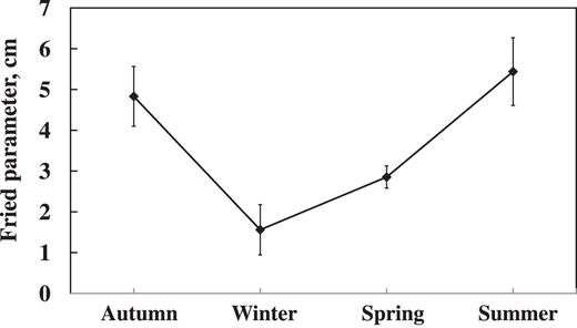
Seasonal behaviours of the daytime Fried parameter (wavelength 535 nm).
Statistics of the Fried parameters.
| Statistics | Autumn | Winter | Spring | Summer |
|---|---|---|---|---|
| Mean | 4.83 | 1.56 | 2.85 | 5.44 |
| Median | 4.64 | 1.39 | 2.80 | 5.22 |
| Standard deviation | 0.37 | 0.31 | 0.135 | 0.52 |
| Statistics | Autumn | Winter | Spring | Summer |
|---|---|---|---|---|
| Mean | 4.83 | 1.56 | 2.85 | 5.44 |
| Median | 4.64 | 1.39 | 2.80 | 5.22 |
| Standard deviation | 0.37 | 0.31 | 0.135 | 0.52 |
Mountain and mountain island sites show a pronounced maximum early in the morning, before ground heating. The temporal seeing at the BAO is shown in Fig. 10, which presents the average Fried parameter as a function of local time. The figure shows the behaviour for 12 September 2015 (t = +15°), where 15 films were collected for every point. The choice of local time on the temporal axis has the advantage of easily showing the seeing conditions during a typical observation day at the BAO. The best seeing is typically encountered after local noon for the ice-free seasons. This stability confirms previous results from the earlier LSVT site-testing campaign. However, significant fluctuations are found on short time-scales, which is typical of daytime turbulence conditions.
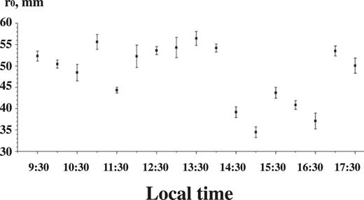
The average Fried parameter as a function of local time (12 September 2015).
We also compared the seasonal V200 trend and solar seeing. Fig. 11 shows the seasonal behaviour during 2015.
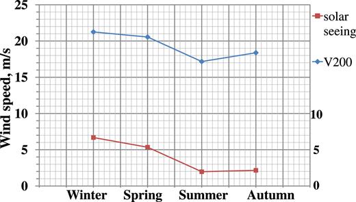
Seasonal behaviour V200 and solar seeing during 2015.
5 CONCLUSIONS
In this study, our aim was to characterize the atmospheric optical daytime turbulence and vertical distribution of wind speed at the BAO, East Siberia, Russia, with the goal of developing AO. We used NCEP/NCAR reanalysis data to provide the vertical distribution of wind speed. The daytime optical turbulence was investigated using the Fried parameter with a S–H WFS in the AO system of the LSVT. Our main results and conclusions are summarized as follows.
Lake Baikal plays an important role in the optical turbulence conditions at the BAO site. The main characteristic is stable ground-layer turbulence throughout the day as a result of the cool waters of Lake Baikal. The best solar seeing conditions, β0 ≈ 1 arcsec, at the BAO are typically encountered in summer on short time-scales. The strongest optical turbulence conditions are detected in winter. Periods of very bad image quality occur in winter, when the Fried parameter is three to four times lower than that in summer; the average value is 1.56 cm and the median value is 1.39 cm at a wavelength of 535 nm, which might be related to the ice regime of Lake Baikal and the high wind speeds during the study period. The strongest wind speeds were observed throughout the atmosphere in winter, while the weakest wind speeds occurred during summer. The maximum daytime Fried parameter was also observed in the summer; the average value is 5.44 cm and the median value is 5.22 cm at a wavelength 535 nm.
For the same period, we also provided wind speed statistics for the 200-mbar level, corresponding to the maximum wind speed values at the jet-stream height. The strongest wind speeds at the 200-mbar level occurred in November (average value 21.41 m s–1 and median value 21.36 m s–1), while the weakest wind speeds were observed in July (average value 10.82 m s–1 and median value 10.54 m s–1). We also found a similar trend between seasonal solar seeing and wind speed at V200 in 2015. Future statistical analyses of the optical turbulence should address this correlation.
Wind speed and optical turbulence distributions determine the bandwidth required for optimal correction with the AO system of a ground-based telescope via a value of Greenwood frequency (equation 2). The combination of strong optical turbulence and wind speeds indicates that the high performance of AO can be complex in winter at the BAO site.
ACKNOWLEDGEMENTS
The authors are grateful to the anonymous referee for valuable remarks that helped to improve and clarify this manuscript. Some of results were obtained using the Unique Research Facility Large Solar Vacuum Telescope and the NCEP/NCAR reanalysis data base. We are grateful to our colleagues L. V. Antoshkin, N. N. Botygina, O. N. Emaleev and P. A. Konyaev for the development of the S–H WFS for AO LSVT. The research was supported by the Russian Science Foundation grant 17-79-20077.
REFERENCES
APPENDIX : SOME EXTRA MATERIAL
Seasonal monthly averages of wind speed from the NCEP/NCAR reanalysis data corresponding to the period 1996–2016.
| P (hPa) | 1 | 2 | 3 | 4 | 5 | 6 | 7 | 8 | 9 | 10 | 11 | 12 | H(m) |
|---|---|---|---|---|---|---|---|---|---|---|---|---|---|
| 925 | 2.85 | 2.37 | 2.23 | 2.23 | 2.26 | 1.94 | 1.48 | 1.48 | 1.67 | 2.07 | 2.94 | 3.17 | 750 |
| 850 | 4.53 | 4.01 | 3.81 | 3.85 | 3.53 | 2.75 | 2.26 | 2.26 | 2.77 | 3.61 | 4.97 | 5.14 | 1 450 |
| 700 | 8.87 | 10.01 | 9.57 | 9.07 | 7.22 | 2.99 | 3.33 | 4.49 | 6.34 | 8.95 | 10.54 | 9.87 | 3 000 |
| 600 | 10.54 | 11.79 | 11.68 | 11.89 | 9.48 | 5.61 | 5.01 | 6.16 | 9.17 | 11.51 | 12.65 | 12.08 | 4 200 |
| 500 | 12.59 | 13.99 | 13.99 | 14.73 | 11.62 | 6.91 | 6.10 | 7.34 | 11.06 | 13.86 | 15.24 | 14.62 | 5 600 |
| 400 | 14.96 | 16.47 | 16.38 | 17.75 | 13.73 | 7.93 | 7.03 | 8.62 | 13.07 | 16.49 | 18.12 | 17.48 | 7 200 |
| 300 | 17.89 | 19.97 | 20.18 | 20.94 | 17.12 | 8.78 | 9.39 | 11.52 | 14.76 | 20.35 | 22.59 | 20.55 | 9 200 |
| 250 | 18.68 | 20.68 | 20.51 | 22.91 | 18.04 | 10.77 | 10.44 | 12.69 | 17.69 | 21.11 | 22.55 | 21.46 | 10 400 |
| 200 | 19.26 | 20.87 | 20.61 | 20.73 | 17.27 | 10.16 | 12.27 | 14.85 | 16.33 | 20.95 | 22.65 | 20.79 | 11 800 |
| 150 | 20.68 | 21.27 | 20.07 | 18.47 | 14.33 | 8.56 | 11.56 | 14.37 | 15.87 | 18.99 | 21.37 | 20.59 | 13 600 |
| 100 | 23.59 | 22.16 | 20.34 | 16.66 | 10.94 | 6.14 | 7.22 | 9.95 | 12.98 | 16.68 | 20.65 | 21.27 | 16 200 |
| 70 | 25.86 | 22.05 | 20.28 | 14.01 | 6.76 | 2.78 | 2.23 | 4.71 | 9.46 | 14.79 | 20.30 | 21.97 | 18 500 |
| 50 | 24.67 | 23.09 | 19.14 | 11.47 | 3.69 | 3.21 | 3.18 | 1.11 | 6.87 | 13.23 | 20.39 | 21.95 | 20 650 |
| 30 | 26.81 | 22.29 | 18.29 | 8.44 | 2.51 | 5.96 | 6.63 | 1.85 | 6.05 | 14.30 | 25.02 | 25.46 | 23 950 |
| 20 | 27.56 | 21.13 | 18.01 | 7.49 | 4.05 | 9.15 | 10.22 | 4.02 | 6.07 | 16.48 | 29.29 | 28.41 | 26 600 |
| 10 | 28.01 | 21.31 | 16.64 | 7.64 | 4.04 | 9.18 | 10.11 | 3.61 | 7.17 | 17.77 | 29.56 | 32.73 | 31 200 |
Mean, median and standard deviation (std) of wind speed at 200 mbar from the NCEP/NCAR reanalysis data for the period 1948–2016.
| Statistics | 1 | 2 | 3 | 4 | 5 | 6 | 7 | 8 | 9 | 10 | 11 | 12 |
|---|---|---|---|---|---|---|---|---|---|---|---|---|
| Mean | 19.49 | 19.33 | 20.13 | 19.92 | 17.39 | 11.77 | 10.82 | 13.98 | 16.18 | 19.52 | 21.41 | 20.48 |
| Median | 19.86 | 19.59 | 20.21 | 19.78 | 17.44 | 11.38 | 10.54 | 13.46 | 16.48 | 19.63 | 21.36 | 20.61 |
| Std | 3.88 | 3.90 | 3.49 | 4.17 | 3.95 | 3.98 | 4.29 | 5.11 | 4.08 | 4.07 | 3.65 | 3.17 |
