


ABSTRACT
The manner in which the stellar initial mass function (IMF) scales with global galaxy properties is under debate. We use two hydrodynamical, cosmological simulations to predict possible trends for two self-consistent variable IMF prescriptions that, respectively, become locally bottom-heavy or top-heavy in high-pressure environments. Both simulations have been calibrated to reproduce the observed correlation between central stellar velocity dispersion and excess mass-to-light ratio (MLE) relative to a Salpeter IMF by increasing the mass fraction of, respectively, dwarf stars or stellar remnants. We find trends of MLE with galaxy age, metallicity, and [Mg/Fe] that agree qualitatively with observations. Predictions for correlations withexces luminosity, half-light radius, and black hole (BH) mass are presented. The significance of many of these correlations depends sensitively on galaxy selection criteria such as age, luminosity, and morphology. For an IMF with a varying high-mass end, some of these correlations are stronger than the correlation with the birth interstellar medium pressure (the property that governs the form of the IMF) because in this case the MLE has a strong age dependence. Galaxies with large MLE tend to have overmassive central BHs. This indicates that the abnormally high MLE observed in the centres of some high-mass galaxies does not imply that overmassive BHs are merely the result of incorrect IMF assumptions, nor that excess M/L ratios are solely the result of overmassive BHs. Satellite galaxies tend to scatter towards high MLE due to tidal stripping, which may have significant implications for the inferred stellar masses of ultracompact dwarf galaxies.
1 INTRODUCTION
The physical interpretation of observational diagnostics of extragalactic stellar populations, as well as predictions for such diagnostics from galaxy formation models, relies on the assumed distribution of masses of stars at birth in a given simple stellar population, the stellar initial mass function (IMF). Such studies often assume a universal functional form, motivated by the apparent universality of the IMF within the Milky Way (MW) galaxy (Kroupa 2001; Chabrier 2003; Bastian, Covey & Meyer 2010).
Recent evidence for IMF variations in the centres of high-mass early-type galaxies challenges this assumption of universality. Some evidence comes from dynamical studies that measure the excess central stellar mass-to-light ratio (MLE) relative to that expected given a fixed IMF. The MLE is typically measured dynamically either via gravitational lensing (e.g. Auger et al. 2010; Treu et al. 2010; Spiniello et al. 2011; Barnabè et al. 2013; Posacki et al. 2015; Smith et al. 2015; Sonnenfeld et al. 2015; Collier, Smith & Lucey 2018) or stellar kinematics (e.g. Thomas et al. 2011; Dutton, Mendel & Simard 2012; Cappellari et al. 2013b; Tortora, Romanowsky & Napolitano 2013; Li et al. 2017), with most studies finding larger values than one would expect for a MW-like IMF. This excess mass may come from excess dim, low-mass, dwarf stars that contribute more to the mass than the light, implying a steeper (bottom-heavy) IMF, or from stellar remnants such as black holes (BHs) or neutron stars, implying a shallower (top-heavy) form. Some information about the functional form of the IMF can be inferred from spectroscopic studies, which indicate that fits to IMF-sensitive stellar absorption features require a larger ratio of dwarf to giant stars, implying that the IMF has a steeper slope either at all masses (e.g. Cenarro et al. 2003; Van Dokkum & Conroy 2010; Spiniello et al. 2012; Ferreras et al. 2013; Spiniello et al. 2014), or only at the low-mass end (e.g. Conroy & van Dokkum 2012; Conroy, van Dokkum & Villaume 2017) or only the high-mass end (e.g. Ferreras et al. 2013; La Barbera et al. 2013; Rosani et al. 2018). Interestingly, observations of local vigorously star-forming galaxies instead imply that the IMF becomes more top-heavy with increasing star formation rate (SFR; Gunawardhana et al. 2011).
The majority of these studies find that the IMF becomes ‘heavier’ with increasing central stellar velocity dispersion, σ. To understand in more detail what drives IMF variations, it is useful to investigate how the IMF varies as a function of other galaxy properties as well. In the observational literature, there seems to be little consensus regarding the correlation between the IMF and galaxy properties other than central σ, the most notable being [Mg/Fe]. Some spectroscopic studies report a strong correlation between the MLE and [Mg/Fe] for early-type galaxies (ETGs), even stronger than that with σ (Conroy & van Dokkum 2012; Smith, Lucey & Carter 2012). On the other hand, the spectroscopic study of La Barbera, Ferreras & Vazdekis (2015) concludes that while the IMF slope correlates with both σ and [Mg/Fe] in stacked SDSS spectra of high-σ ETGs, the correlation with [Mg/Fe] vanishes at fixed σ. The dynamical study of McDermid et al. (2014) finds a significant (but weak) trend of MLE with [Mg/Fe] for ATLAS3D galaxies that, however, does not appear to be as strong as the correlation with σ (Cappellari et al. 2013b). Smith (2014) shows that studies that employ dynamical methods tend to favour trends between σ with little [Mg/Fe] residual dependence, while spectroscopic methods favour a [Mg/Fe] correlation with no residual σ dependence, even when applied to the same galaxy sample.
The situation is even more uncertain for trends between the IMF and stellar metallicity. Spatially resolved spectroscopic IMF studies have found that the IMF correlates strongly with local stellar metallicity (Martín-Navarro et al. 2015a; Conroy et al. 2017), while global trends tend to be weaker, with spectroscopic studies finding only weak trends (Conroy & van Dokkum 2012), and dynamical studies finding no significant correlation at all (McDermid et al. 2014; Li et al. 2017). These discrepancies between the IMF scalings among observational IMF studies are often chalked up to differences in modelling procedures and unknown systematic biases (Clauwens, Schaye & Franx 2015). Clauwens, Schaye & Franx (2016) showed that given the uncertain observational situation, the consequences of the inferred IMF variations for the interpretation of observations of galaxy populations could vary from mild to dramatic.
Recently, Barber, Crain & Schaye (2018, hereafter Paper I) presented a suite of cosmological, hydrodynamical simulations that self-consistently vary the IMF on a per-particle basis as a function of the interstellar medium (ISM) pressure from which star particles are born. These simulations, which adopt, respectively, a bottom-heavy and a top-heavy IMF, use the EAGLE model for galaxy formation (Schaye et al. 2015). They reproduce the observed |$z$| ≈ 0 galaxy luminosity function, half-light radii, and BH masses, and the IMF dependence on pressure has been calibrated to reproduce the observed MLE−σ relation. The goal of this paper is to determine, for the first time, the relationships between the IMF and global galaxy properties that arise from a self-consistent, hydrodynamical, cosmological model of galaxy formation and evolution with calibrated IMF variations. In doing so, we can inform on the differences (and similarities) in such relationships as a result of differences in IMF parametrizations.
This paper is organized as follows. In Section 2, we summarize the variable IMF simulations. Section 3 shows the circumstances for which the MLE is a reasonable tracer of the IMF. Section 4 shows the resulting correlations between the MLE and various galaxy properties, including age, metallicity, [Mg/Fe] stellar mass, luminosity, and size. Section 4.5 shows how galaxies with overmassive BHs tend to also have a high MLE. Section 4.6 investigates which observables most closely correlate with MLE. Section 5 examines the environmental effects on the MLE−σ relation. We summarize in Section 6. In a future work (Paper III), we will discuss the spatially resolved IMF trends within individual galaxies, including the effect of a variable IMF on radial abundance gradients as well as on the MLE−σ relation at high redshift. These simulations are publicly available at http://icc.dur.ac.uk/Eagle/database.php (McAlpine et al. 2016).
2 SIMULATIONS
In this paper, we investigate IMF scaling relations using cosmological, hydrodynamical simulations that self-consistently vary the IMF on a per-particle basis. These simulations were presented in Paper I and are based on the EAGLE model (Crain et al. 2015; Schaye et al. 2015; McAlpine et al. 2016). Here, we give a brief overview of EAGLE and the modifications made to self-consistently implement variable IMF prescriptions. We refer the reader to Schaye et al. (2015) and Paper I for further details.
The simulations were run using a heavily modified version of the Tree-PM smooth particle hydrodynamics code gadget-3 (Springel 2005), on a cosmological periodic volume of (50 Mpc)3 with a fiducial ‘intermediate’ particle mass of |$m_{\rm g} = 1.8 \times 10^6\, \, {\rm M_{\odot }}$| and |$m_{\rm DM} = 9.7\times 10^{6}\, \, {\rm M_{\odot }}$| for gas and dark matter, respectively. The gravitational softening length was kept fixed at 2.66 comoving kpc prior to |$z$| = 2.8, switching to a fixed 0.7 proper kpc thereafter. Cosmological parameters were chosen for consistency with Planck 2013 in a Lambda cold dark matter cosmogony (Ωb = 0.04825, Ωm = 0.307, ΩΛ = 0.693, h = 0.6777; Planck Collaboration I 2014).
The reference EAGLE model employs analytical prescriptions to model physical processes that occur below the resolution limit of the simulation (referred to as ‘subgrid’ physics). The 11 elements that are most important for radiative cooling and photoheating of gas are tracked individually through the simulation, with cooling and heating rates computed according to Wiersma, Schaye & Smith (2009a) subject to an evolving, homogeneous UV/X-ray background (Haardt & Madau 2001). Once gas particles reach a metallicity-dependent density threshold that corresponds to the transition from the warm, atomic to the cold, molecular gas phase (Schaye 2004), they become eligible for stochastic conversion into star particles at a pressure-dependent SFR that reproduces the Kennicutt–Schmidt star formation law (Schaye & Dalla Vecchia 2008). Star particles represent coeval simple stellar populations that, in the reference model, adopt a Chabrier (2003) IMF. They evolve according to the lifetimes of Portinari, Chiosi & Bressan (1997), accounting for mass-loss from winds from massive stars and AGB stars, as well as supernovae (SNe) Types II and Ia (Wiersma et al. 2009b). Stellar ejecta are followed element-by-element and are returned to the surrounding ISM, along with thermal energetic stellar feedback (Dalla Vecchia & Schaye 2012) whose efficiency was calibrated to match the |$z$| ≈ 0 galaxy stellar mass function (GSMF) and galaxy sizes. Supermassive BHs are seeded in the central regions of high-mass dark matter haloes and grow via accretion of low angular momentum gas (Springel, Di Matteo & Hernquist 2005; Booth & Schaye 2009; Rosas-Guevara et al. 2015) and mergers with other BHs, leading to thermal, stochastic active galactic nucleus (AGN) feedback (Schaye et al. 2015) that acts to quench star formation in high-mass galaxies.
The two simulations used in this study use the same subgrid physics prescriptions as the reference EAGLE model, except that the IMF is varied as a function of the pressure of the ISM from which individual star particles form. To ensure that the simulations remain self-consistent, the stellar mass-loss, nucleosynthetic element production, stellar feedback, and star formation law are all modified to be consistent with the IMF variations (see Paper I for details). The variable IMF simulations have the same volume, initial conditions, and resolution as the Ref-L050N0752 (hereafter referred to as Ref-50) simulation of Schaye et al. (2015).
Our two variable IMF simulations differ only in their prescriptions for the IMF. In the first, which we refer to as LoM-50, the low-mass slope of the IMF (from 0.1 to |$0.5\, \, {\rm M_{\odot }}$|) is varied, while the slope at higher masses remains fixed at the Kroupa (2001) value of −2.3. In this prescription, the IMF becomes bottom-heavy in high-pressure environments, with the slope ranging from 0 to −3 in low- and high-pressure environments, respectively, transitioning smoothly between the two regimes via a sigmoid function over the range |$P/k_B \approx 10^4\!-\!10^6\, {\rm K}\, {\rm cm}^{-3}$|. Such a prescription produces stellar populations with larger stellar M/L ratios at high pressures due to an excess mass fraction of low-mass dwarf stars that contribute significantly to the mass but not to the light.
For the second simulation, hereafter HiM-50, we instead keep the low-mass slope fixed at the Kroupa value of −1.3 and vary the high-mass slope (from 0.5 to |$100 \, {\rm M_{\odot }}$|) from −2.3 to −1.6 with increasing birth ISM pressure, transitioning smoothly over the same pressure range as in the LoM-50 simulation. This prescription increases the M/L relative to a Kroupa IMF at high pressures by increasing the mass fraction of short-lived high-mass stars, resulting in a larger fraction of stellar remnants such as BHs, neutron stars, and white dwarfs, and lower luminosity once these high-mass stars have died off (after a few |$100\, {\rm Myr}$|). Note that varying the IMF with pressure is essentially equivalent to varying it with SFR surface density since the latter is determined by the former in the EAGLE model.
These IMF parametrizations were individually calibrated to match the observed trend between the MLE and central stellar velocity dispersion found by Cappellari et al. (2013b) for high-mass elliptical galaxies. This calibration was done in post-processing of the reference (100 Mpc)3 EAGLE model (Ref-L100N1504) using the Flexible Stellar Population Synthesis (fsps) software package (Conroy, Gunn & White 2009; Conroy & Gunn 2010). Specifically, the allowed range of IMF slopes and the pressure range over which the IMF gradually transitions from one slope to the other were tuned until an acceptable qualitative match to the Cappellari et al. (2013b) trend was obtained. We refer the reader to Paper I for further details on the calibration procedure. In Paper I, we verified that the variable IMF runs reproduce the Cappellari et al. (2013b) trend between the MLE and velocity dispersion, but we also demonstrated that calibrating the IMF to reproduce that trend does not guarantee a match to other observational constraints on the IMF, such as the dwarf-to-giant ratio in ETGs or the ratio of ionizing to UV flux in star-forming galaxies.
In Paper I, we also showed that our variable IMF simulations maintain agreement with the observables used to calibrate the EAGLE model: the present-day galaxy luminosity function, the relations between galaxy luminosity and half-light radius and BH mass, and the global rate of Type Ia SNe. This result may seem surprising given that the IMF governs the strength of stellar feedback to which these calibration observables are quite sensitive (Crain et al. 2015). The fact that these galaxy observables are not strongly affected by the modified stellar feedback is likely due to the following (simplified) picture, which we separate into star-forming and quenched regimes.
If galaxy formation is self-regulated and if the outflow rate is large compared with the SFR rate, then the outflow rate will tend to adjust to balance the inflow rate when averaged over sufficiently long time-scales. If we neglect preventative feedback and recycling, then the gas inflow rate tracks that of the dark matter and does not depend on the IMF. If the IMF is modified, then a star-forming galaxy of fixed mass will adjust its SFR to ensure that the same feedback energy is released in order to generate the same outflow rate that is needed to balance the inflow rate. For a top-heavy IMF, galaxies need to form fewer stars relative to the case of a standard IMF to obtain the same feedback energy. This results in lower SFRs, and thus lower ratios of stellar mass to halo mass, resulting in a lower normalization of the GSMF. However, for star-forming galaxies, M/L is lower due to the top-heavy IMF, so the luminosity at fixed halo mass ends up being similar to the Chabrier case. According to Booth & Schaye (2010) and Bower et al. (2017), BH mass is a function of halo mass (for sufficiently large halo masses) for a fixed AGN feedback efficiency, so the MBH−L relation is also not strongly affected. For a bottom-heavy IMF, this situation is reversed, where more stars are required to obtain the same feedback energy, increasing the GSMF, but their higher M/L ratios (due to an increased fraction of dwarf stars) makes the luminosity function (and the MBH−L relation) similar to the Chabrier case.
For low-mass galaxies these effects are small in our simulations since the IMF only varies away from Chabrier at the high pressures typical of high-mass galaxies. In the latter regime, AGN feedback quenches galaxies at a particular virial temperature (or rather entropy; Bower et al. 2017), leading to an approximately fixed BH mass–halo mass relation (because MBH must be sufficiently high to drive an outflow and quench star formation). For a top-heavy IMF, the lower M⋆/M200 (assuming the stellar mass formed while the galaxy was star-forming) leads to higher MBH/M⋆ and a lower GSMF. A quenched galaxy with a top-heavy IMF can have a higher or lower M/L depending on how long it has been quenched – if quenched for more than ≈3 Gyr, M/L is higher so the luminosity function cuts off at lower luminosity. However, since high-mass galaxies are not as strongly quenched in HiM-50, this effect is small. For a bottom-heavy IMF, everything is reversed: galaxies are quenched at higher M⋆, leading to a higher GSMF, but since M/L is higher, they quench at lower luminosity so the luminosity function remains similar.
In the intermediate-mass regime (around the knee of the GSMF), the situation is more complex since both stellar feedback and AGN feedback play an important role in self-regulation and the star formation law becomes important (see Paper I). As noted above, a top-heavy IMF leads to a lower SFR because of the larger amount of feedback energy per unit stellar mass formed. This would imply a lower gas fraction, which would reduce the BH growth. However, this effect is counteracted by the decreased normalization of the observed star formation law at high pressures (relative to that of a standard IMF), which increases the gas surface densities at fixed SFR surface density. Thus, AGN feedback and BH growth are not strongly affected at fixed halo mass and galaxy luminosity. Again, the situation is reversed for bottom-heavy IMF variations. These effects, as well as the relatively poor statistics at the high-mass end relative to the (100 Mpc)3 EAGLE simulation, likely eliminated any need to adjust the feedback parameters originally used to calibrate the EAGLE model.
Structures in the simulation are separated into ‘haloes’ using a friends-of-friends halo finder with a linking length of 0.2 times the mean interparticle spacing (Davis et al. 1985). Galaxies are identified within haloes as self-bound structures using the subfind algorithm (Springel et al. 2001; Dolag et al. 2009). We consider only galaxies with at least 500 stellar particles, corresponding to a stellar mass |$M_{\star }\approx 9 \times 10^{8} \, {\rm M_{\odot }}$|. Galaxies in the mass range of interest in this study are sufficiently well resolved, as those with |$\sigma _e \gt 80\, {\rm km}\, {\rm s}^{-1}$| have |$M_{\star }\gt 10^{10} \, {\rm M_{\odot }}$|, corresponding to ≳5600 stellar particles. Unless otherwise specified, all global galactic properties shown in this paper (e.g. MLE, age, metallicity, [Mg/Fe]) are computed considering star particles within the 2d projected half-light radius, re, of each galaxy, measured with the line of sight parallel to the z-axis of the simulation box.
3 IS THE (M/L)-EXCESS A GOOD TRACER OF THE IMF?
In Fig. 1, we show MLEr as a function of IMF slope for galaxies with |$\sigma _e \gt 80\, {\rm km}\, {\rm s}^{-1}$| in our variable IMF simulations at |$z$| = 0.1, coloured by age. For LoM-50, MLEr is an excellent tracer of the IMF, with very little dependence on age or metallicity. For HiM-50, MLEr is only a good tracer of the IMF at fixed age (and, ideally, old age since the slope is very shallow for ages |${\lesssim } 3\,$| Gyr), as can be seen by the strong vertical age gradient (i.e. the colour of the data points) at fixed high-mass slope in the right-hand panel.
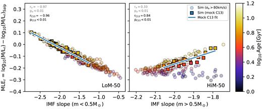
Excess r-band mass-to-light ratio relative to that for a Salpeter IMF as a function of IMF slope for galaxies with |$\sigma _e \gt 10^{1.9}\ (\approx\! 80)\, {\rm km}\, {\rm s}^{-1}$| at |$z$| = 0.1, coloured by stellar age. All quantities are r-band light-weighted means measured within the 2D projected r-band half-light radius. The left-hand and right-hand panels show low-mass (|$m \lt 0.5 \, {\rm M_{\odot }}$|) and high-mass (|$m \gt 0.5 \, {\rm M_{\odot }}$|) IMF slopes for LoM-50 and HiM-50, respectively. Galaxies selected in a similar way to C13 (see text) are shown as opaque squares, while all others are shown as the translucent circles. The Pearson correlation coefficient, r, and its p-value are indicated in each panel for the |$\sigma _e \gt 10^{1.9}\, {\rm km}\, {\rm s}^{-1}$| and mock C13 samples in grey and black, respectively. The blue solid lines show least-squares fits to the mock C13 samples (see Table 1). MLEr is an excellent proxy for the low-mass IMF slope variations but is only a good proxy for high-mass slope variations for old galaxies, with age-dependent scatter.
To compare our results with observed trends between MLEr and galaxy properties in the literature, we select galaxies from our simulations using approximately the same selection criteria as the ATLAS3D sample used by Cappellari et al. (2013b, hereafter C13). Their galaxy sample is complete down to MK = −21.5 mag, consisting of 260 morphologically selected elliptical and lenticular galaxies, chosen to have old stellar populations (H β equivalent width less than |$2.3 \buildrel_\circ \over {\mathrm{A}}$|). For our ‘mock C13’ sample, we select galaxies with MK < −21.5 mag and intrinsic u* − r* > 2. The u* − r* colour cut roughly separates galaxies in the red sequence from the blue cloud for EAGLE galaxies (Correa et al. 2017) and ensures that we exclude galaxies with light-weighted ages younger than ≈3 Gyr.
The mock C13 galaxies are highlighted as the opaque squares in Fig. 1. Since these galaxies are selected to be older than |${\approx } 3\, {\rm Gyr}$|, their MLE is a reasonable tracer of the IMF in HiM-50 but with more scatter than for LoM-50 due to the residual age dependence.2 These dependencies should be kept in mind when interpreting the trends between the MLEr and global galaxy properties shown in the next section.
4 TRENDS BETWEEN THE (M/L)-EXCESS AND GLOBAL GALACTIC PROPERTIES
There is currently much debate regarding possible trends between the IMF and global galaxy properties other than velocity dispersion, such as age, metallicity, and alpha enhancement. In this section, we investigate these trends in our (self-consistent, calibrated) variable IMF simulations, where the IMF is governed by the local pressure in the ISM. In the left-hand and right-hand columns of Fig. 2, we show MLEr as a function of these properties in LoM-50 and HiM-50, respectively, and compare with observed trends for ETGs from the ATLAS3D survey (McDermid et al. 2014) and another sample from Conroy & van Dokkum (2012). Note that while McDermid et al. (2014) measure MLE within a circular aperture of radius re, they (as well as Conroy & van Dokkum 2012)3 measure age, metallicity, and [Mg/Fe] within re/8. For many of our galaxies, re/8 would be close to the gravitational softening scale of the simulation. Indeed, performing our analysis within this aperture only serves to add resolution-related noise to the plots. Thus, since McDermid et al. (2014) claim that their results are unchanged for an aperture choice of re, we report our results consistently within re. For completeness, we show all galaxies with |$\sigma _e \gt 10^{1.9}\ (\approx 80)\, {\rm km}\, {\rm s}^{-1}$| (the σe-complete sample; translucent circles) but focus our comparison with observations on galaxies consistent with the C13 selection criteria (opaque squares). This σe limit of |$80\, {\rm km}\, {\rm s}^{-1}$| was chosen because it is the lowest σe value that our mock C13 samples reach.
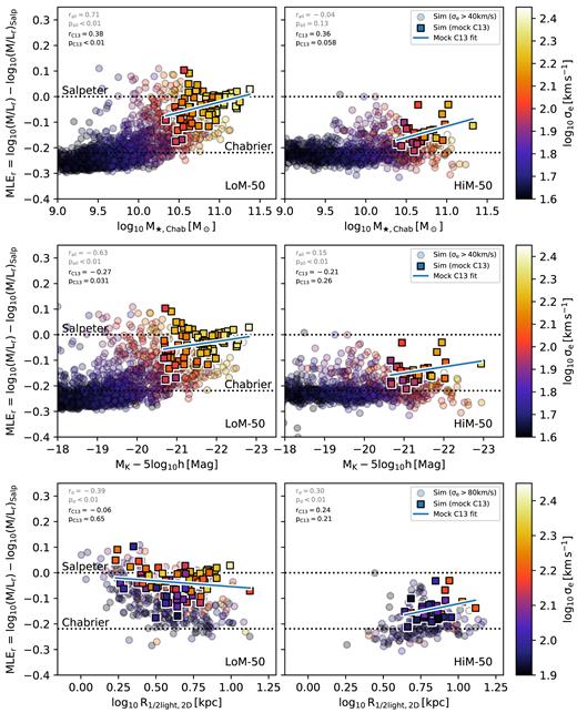
![Excess r-band M/L-ratio with respect to that for a Salpeter IMF (MLEr) as a function of r-band light-weighted mean age (top row), stellar metallicity (middle row), and stellar alpha-enhancement (bottom row), for galaxies with $\sigma _e \gt 10^{1.9}\ (\approx 80)\, {\rm km}\, {\rm s}^{-1}$ in the LoM-50 (left-hand column) and HiM-50 (right-hand column) simulations at $z$ = 0.1. Points are coloured by σe. All quantities are computed within (2D-projected) re. Galaxies selected in a similar way to C13 (see text) are shown as the opaque squares, while all others are shown as the translucent circles. The blue solid lines show least-squares fits to the mock C13 samples (see Table 1). The simulation values for [Mg/Fe] have been increased by 0.3 dex for LoM-50. We assume Z⊙ = 0.127 and take other solar abundances from Asplund et al. (2009). We show the linear fits with 1σ scatter found in McDermid et al. (2014) as the green-solid and -dashed lines, respectively, and the MLE−[Mg/Fe] relation of Conroy & van Dokkum (2012) as the cyan triangles. Metallicities from McDermid et al. (2014) have been converted to our solar scale. For both variable IMF simulations, we see strong positive correlations of MLEr with age and [Mg/Fe]. When considering all galaxies with $\sigma _e \gt 80\, {\rm km}\, {\rm s}^{-1}$, we find a weak but significant negative correlation with Z for both simulations, but the correlation disappears for mock C13 galaxies.](https://oup.silverchair-cdn.com/oup/backfile/Content_public/Journal/mnras/482/2/10.1093_mnras_sty2825/2/m_sty2825fig2.jpeg?Expires=1749848650&Signature=EpSkO9D9aw67qzFkS5556Nsb7gldl-zj~uk2tB5bxoKFSYA8dnA4jy5AuF89WouIw6Mp1pnYpnMqiIGamBKQGW-wGm8A3q8f7ORuD-qUIRKm0pSwTUFV4h8xP09PcjaG4Y8-yjVg7Rza1zuQcg0MbY83guDSsJO4T8ElNfce6arD49lnE0Pl5bCgpX~9o84tgWQTKnb~2tn87HsjZ-7t6H7kGkxDyOylgIFMoBLmirIJWj~yZU7CyQrA9DpTCEKB5HY~YB5uJTxpFB5kj92PylbVMY2f7~R7KeNpJJRpwQXGtSCv2mC-V8lTI-pZukL9cDOpa0HfHb-5y-a278KzjA__&Key-Pair-Id=APKAIE5G5CRDK6RD3PGA)
Excess r-band M/L-ratio with respect to that for a Salpeter IMF (MLEr) as a function of r-band light-weighted mean age (top row), stellar metallicity (middle row), and stellar alpha-enhancement (bottom row), for galaxies with |$\sigma _e \gt 10^{1.9}\ (\approx 80)\, {\rm km}\, {\rm s}^{-1}$| in the LoM-50 (left-hand column) and HiM-50 (right-hand column) simulations at |$z$| = 0.1. Points are coloured by σe. All quantities are computed within (2D-projected) re. Galaxies selected in a similar way to C13 (see text) are shown as the opaque squares, while all others are shown as the translucent circles. The blue solid lines show least-squares fits to the mock C13 samples (see Table 1). The simulation values for [Mg/Fe] have been increased by 0.3 dex for LoM-50. We assume Z⊙ = 0.127 and take other solar abundances from Asplund et al. (2009). We show the linear fits with 1σ scatter found in McDermid et al. (2014) as the green-solid and -dashed lines, respectively, and the MLE−[Mg/Fe] relation of Conroy & van Dokkum (2012) as the cyan triangles. Metallicities from McDermid et al. (2014) have been converted to our solar scale. For both variable IMF simulations, we see strong positive correlations of MLEr with age and [Mg/Fe]. When considering all galaxies with |$\sigma _e \gt 80\, {\rm km}\, {\rm s}^{-1}$|, we find a weak but significant negative correlation with Z for both simulations, but the correlation disappears for mock C13 galaxies.
4.1 MLE versus age
First, we investigate the relationship between the MLE and galaxy age. In the top row of Fig. 2, we show MLEr as a function of the Lr-weighted mean stellar age of galaxies in LoM-50 (left-hand panel) and HiM-50 (right-hand panel). For both simulations, we see a strong trend of increasing MLEr with age, where older galaxies tend to have higher (i.e. heavier) MLEr. This result is in qualitative agreement with McDermid et al. (2014) but with a steeper slope for LoM-50, and smaller scatter for HiM-50. Note as well that the positive trend found by McDermid et al. (2014) is sensitive to the methodology used, and in fact disappears when (M/Lr)Salp is derived from individual line strengths rather than full spectral fitting. It is thus quite interesting that we find strong positive correlations with age for both simulations.
For LoM-50, this trend is driven by the higher pressures at which stars form at higher redshift (as was shown for Ref-50 by Crain et al. 2015 and will be investigated further for our simulations in Paper III), yielding more bottom-heavy IMFs for older ages. For HiM-50, the trend with age is tighter due to the fact that, in addition to the trend of higher birth ISM pressure with increasing formation redshift, the MLEr increases with age for a stellar population with a top-heavy IMF, even if the IMF is fixed. The result is that, even though the IMF itself depends only on birth ISM pressure, in the end the MLEr correlates more strongly with age than with IMF slope (compare the upper right-hand panel of Fig. 2 with the right-hand panel of Fig. 1; also fig. 2 of Paper I). This is especially true for the σe-complete sample due to its large range of ages, while the age dependence is reduced for the mock C13 sample due to the exclusion of young galaxies.
We also note that galaxies with |$\sigma _e\gt 80\, {\rm km}\, {\rm s}^{-1}$| in HiM-50 extend to quite young ages (<1 Gyr), whereas in the LoM-50 case only a handful of galaxies are <3 Gyr old (although the u* − r* selection criterion removes all galaxies with light-weighted ages younger than 3 Gyr in our mock C13 samples). This age difference is due to the higher SFRs in the HiM-50 simulation relative to LoM-50, which were discussed in Paper I. We remind the reader that we ignore the luminosities of star particles with ages less than 10 Myr. Without this cut, the age and MLEr would extend to even lower values due to the ongoing star formation in HiM-50 galaxies.
We conclude that both LoM-50 and HiM-50 agree qualitatively with the positive trend of MLEr with age inferred from the ATLAS3D survey by McDermid et al. (2014), but with a stronger correlation. We encourage other observational IMF studies to measure the correlation between IMF diagnostics and age as well in order to help test these predictions.
4.2 MLE versus metallicity
Observationally, evidence for trends between the IMF and metal abundances have been reported, but with conflicting results. While spectroscopic studies find strong positive trends of bottom-heaviness with local metallicity (Martín-Navarro et al. 2015a; Conroy et al. 2017), dynamical studies find no significant correlation between MLEr and global metallicity (McDermid et al. 2014; Li et al. 2017). In the middle row of Fig. 2, we plot MLEr versus (dust-free) Lr-weighted metallicity measured within re. We assume Z⊙ = 0.0127 and convert observationally derived metallicities from the literature to this scale. The offset of HiM-50 galaxies towards higher metallicities is due to the higher nucleosynthetic yields resulting from a top-heavy IMF, as discussed in Paper I.
For both variable IMF simulations, we see a weak but significant trend of decreasing MLEr with metallicity for the sample with |$\sigma \gt 80\, {\rm km}\, {\rm s}^{-1}$|. For both LoM-50 and HiM-50, the negative correlation of MLEr with metallicity is a consequence of the positive and negative relationships of the MLEr and Z, respectively, with age. Interestingly, in HiM-50 the negative correlation with metallicity is weaker than in LoM-50 despite the stronger dependence of MLEr on age. This is the result of the strong effect that a top-heavy IMF has on the metal yields. At fixed age, a galaxy with higher MLE has on average an IMF with a shallower high-mass slope, resulting in higher metal yields and thus higher metallicities. The effect is strongest for the oldest galaxies where the scatter in MLEr is greatest (see upper right-hand panel of Fig. 2). Thus, the oldest galaxies with high MLEr that would have had low metallicity with a Chabrier IMF get shifted towards higher metallicity in the middle right-hand panel of Fig. 2, reducing the strength of the negative MLEr−Z correlation.
Restricting our sample to the mock C13 galaxies, the negative trend with Z is weaker and no longer significant for LoM-50 and is weakly positive for HiM-50. The negative trend for HiM-50 disappears for this sample because we remove the low-metallicity, old galaxies with intermediate MLE that help drive the negative trend in the σe-complete selection. These galaxies are excluded from the mock C13 selection due to the luminosity cut. The weakness of these trends is in agreement with the weakly negative but non-significant correlation of McDermid et al. (2014) as well as the lack of correlation found by Li et al. (2017). Interestingly, our results are in stark contrast with the positive correlation between the IMF slope and spatially resolved local metallicity of Martín-Navarro et al. (2015a). We make a fairer comparison to their result in Paper III, where we show that locally we do in fact find a positive correlation between MLEr and metallicity.
We conclude that, for a σe-complete sample of galaxies, the MLEr is predicted to anticorrelate with total stellar metallicity for low-mass IMF slope variations, while being relatively insensitive to metallicity for high-mass slope variations. In both cases, these correlations disappear for samples consistent with the selection criteria of the ATLAS3D survey, in agreement with dynamical studies.
4.3 MLE versus [Mg/Fe]
In the bottom row of Fig. 2, we plot MLEr as a function of [Mg/Fe],4 both measured within re. For LoM-50, we increase the [Mg/Fe] values by 0.3 dex to facilitate comparison with the observed trends. This procedure is somewhat arbitrary, but is motivated by the fact that Segers et al. (2016) showed that [Mg/Fe] is underestimated by EAGLE and that the nucleosynthetic yields are uncertain by about a factor of 2 (Wiersma et al. 2009b); thus the slopes of these trends are more robust than the absolute values. This procedure is not necessary for HiM-50 due to the increased metal production resulting from a top-heavy IMF (see fig. 9 of Paper I).
For both simulations, for the |$\sigma _e\gt 80\, {\rm km}\, {\rm s}^{-1}$| selection we see weak but significant positive correlations between MLEr and [Mg/Fe]. When selecting only mock C13 galaxies, the trend for LoM-50 is still positive but no longer significant. These trends are in qualitative agreement with the positive trends found by Conroy & van Dokkum (2012) and McDermid et al. (2014) and highlight the importance of sample selection in determining the significance of these correlations. For HiM-50, the MLEr−[Mg/Fe] relation is stronger than in LoM-50, likely due to a combination of the fact that [Mg/Fe] correlates strongly with age in high-mass galaxies (Segers et al. 2016) and the fact that the [Mg/Fe] ratios are strongly affected by the shallow high-mass IMF slopes resulting from the HiM IMF parametrization (see Paper I). The correlation strengthens for the mock C13 selection due to the exclusion of young, blue galaxies with intermediate [Mg/Fe] values, although given the low number of high-[Mg/Fe] mock C13 galaxies in HiM-50, the strength of this correlation may be sensitive to our mock C13 selection criteria.
In Section 4.6, we show that the trend between MLEr and [Mg/Fe] for LoM-50 galaxies is solely due to the correlation between [Mg/Fe] and σe, while that for HiM-50 is partially due to the correlation between [Mg/Fe] and age. The former is consistent with La Barbera et al. (2015) who found that, while the observations are consistent with a correlation between MLE and [Mg/Fe], this correlation disappears at fixed central velocity dispersion.
4.4 MLE versus Chabrier-inferred galaxy mass, luminosity, and size
In order to build intuition on how the IMF varies from galaxy to galaxy, it is also useful to predict trends between the MLE and other basic galactic properties that have not yet been investigated observationally. In Fig. 3, we show the MLEr as a function of, from top to bottom, Chabrier-interpreted stellar mass (M⋆,Chab), K-band luminosity, and 2D projected half-light radius for LoM-50 (left-hand column) and HiM-50 (right-hand column) for all galaxies with σe > 101.6 km s−1, coloured by σe. Note that we now include galaxies of lower σe than in Fig. 2 to facilitate comparison with the MLEr−σe relation shown in fig. 5 of Paper I and to show the full transition from Chabrier-like to bottom- or top-heavy IMFs over a wide range of masses and luminosities. Those that would be selected by ATLAS3D (i.e. are in our mock C13 samples) are shown as the opaque squares, while others are shown as the translucent circles. M⋆,Chab is computed by multiplying each galaxy’s K-band luminosity by the stellar M/LK that it would have had if its stellar populations had evolved with a Chabrier IMF (given the same ages and metallicities). Note that this is still not exactly the same as would be inferred observationally, as it does not take into account possible biases in the inferred ages or metallicities due to IMF variations.
As Fig. 2 but now showing M/Lr excess as a function of, from top to bottom, stellar mass reinterpreted assuming a Chabrier IMF, K-band absolute magnitude, and projected r-band half-light radius. For completeness, we include all galaxies with |$\sigma _e \gt 10^{1.6} (\approx 40)\, {\rm km}\, {\rm s}^{-1}$| in the upper two rows, while the lower row shows galaxies with |$\sigma _e \gt 10^{1.9} (\approx 80)\, {\rm km}\, {\rm s}^{-1}$|. We see roughly the same trends of MLEr with M⋆,Chab and MK as with σe (see fig. 5 of Paper I), but with greater scatter. In LoM-50, smaller high-σe galaxies tend to form the more bottom-heavy populations, while larger counterparts form the more top-heavy populations in HiM-50.
The top row shows MLEr as a function of M⋆,Chab. For LoM-50, we see a strong trend of increasing bottom-heaviness with mass for galaxies with |$M_{\rm \star ,Chab}\gt 10^{10} \, {\rm M_{\odot }}$|. Galaxies below this limit tend to have Chabrier-like IMFs. The scatter here is stronger than in the MLEr−σe relation, leading to a somewhat weaker correlation of MLEr with M⋆,Chab for LoM-50. In agreement with Clauwens et al. (2015), galaxies in our mock C13 sample are only complete down to |$M_{\rm \star ,Chab}\approx 10^{10.5} \, {\rm M_{\odot }}$|, much higher than the |$6\times 10^{9} \, {\rm M_{\odot }}$| quoted by Cappellari et al. (2013a). For HiM-50, it is only for the mock C13 galaxies that we see even a weakly positive relation between MLEr and M⋆,Chab due to a bias towards high-MLE galaxies at high mass due to the cut in u* − r*: at fixed mass, galaxies with low MLE tend to be younger, and thus bluer, and are more likely to be excluded from our mock C13 sample. However, in contrast to the significant, positive MLEr−σe correlation for this sample, this positive MLEr−M⋆,Chab relation for mock C13 HiM-50 galaxies is not significant and may be sensitive to the way in which mock C13 galaxies are selected. Note that using true M⋆ on the x-axis rather than M⋆,Chab would shift the highest-MLE galaxies to larger mass by ≈0.2−0.3 dex, and using Salpeter-inferred M⋆ would shift all points systematically to higher mass by 0.22 dex, neither of which would make any difference to these results.
The middle row of Fig. 3 shows MLEr as a function of K-band absolute magnitude. For both simulations, the trend is very similar to that with M⋆,Chab but with a shallower slope (in this case the positive relation between the MLEr and luminosity yields a negative Spearman r for the correlation with magnitude).
The bottom row shows MLEr as a function of 2D projected r-band half-light radius, re. In this row, we show only galaxies with |$\sigma _e \gt 10^{1.9}\, {\rm km}\, {\rm s}^{-1}$| (as in Fig. 2) to remove the high number of low-mass galaxies with Chabrier-like IMFs that would reduce the significance of any correlation. Here, the two simulations show markedly different behaviour. While MLEr decreases with re for LoM-50, it increases for HiM-50. To help explain this behaviour, we plot in Fig. 4 the re−σe relation for each simulation, coloured by MLEr (note that this figure contains the same information as the bottom row of Fig. 3). For HiM-50 (right-hand panel), we see a positive correlation between re and σe, with no noticeable gradient in MLEr at fixed σe. Thus, for HiM-50 the MLEr−re relation matches qualitatively the MLEr−σe relation.
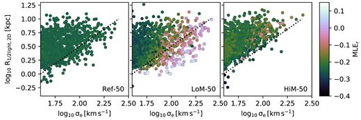
Effect of IMF variations on the relation between r-band half-light radius and σe. We show all galaxies with |$\sigma _e \gt 10^{1.6}\, {\rm km}\, {\rm s}^{-1}$| at |$z$| = 0.1 in, from left to right, Ref-50, LoM-50, and HiM-50, respectively. Points are coloured by MLEr. The same (arbitrary) dotted line is repeated in each panel to guide the eye. Galaxies that are smaller at fixed σe have larger MLEr in LoM-50. In HiM-50, the re−σe relation is tighter, likely due to the stronger feedback in high-pressure (i.e. top-heavy IMF) environments.
In the middle panel of Fig. 4, we see that, as in HiM-50, LoM-50 galaxies increase in size with increasing σe, but they also exhibit stronger scatter in the re−σe relation towards smaller galaxies. There is a strong MLEr gradient at fixed σe here, where, at fixed σe, smaller galaxies tend to have larger MLEr, resulting in a negative correlation between MLEr and re at fixed σe. This anticorrelation counteracts the (positive) MLEr−σe relation, resulting in a net negative correlation between MLEr and re for the σe-complete sample in LoM-50 (lower left-hand panel of Fig. 3). Interestingly, the trend disappears for the mock C13 sample as many of the smallest (and thus highest MLEr) high-σe galaxies are excluded due to the luminosity cut, causing these two effects (positive MLEr−σe relation coupled with negative MLEr−re at fixed σe) to roughly cancel out.
This behaviour can be explained by the impact of these variable IMF prescriptions on feedback, and thus re, at fixed σe. In both cases, galaxies that are smaller at fixed σe tend to have formed their stars at higher pressures, giving them larger MLEr values. In LoM-50, such galaxies experience weaker feedback due to their bottom-heavy IMFs, further decreasing their sizes relative to galaxies of similar σe in Ref-50 (compare the middle and left-hand panels of Fig. 4). The behaviour is different for HiM-50 due to the fact that galaxies that form at high pressure instead experience stronger feedback due to the top-heavy IMF. This enhanced feedback increases their sizes due to the increased macroscopic efficiency of the ejection of low-angular momentum gas, pushing them upward in the right-hand panel of Fig. 4 (or to the right in the lower right-hand panel of Fig. 3). Interestingly, this feedback effect tightens the relationship between re and σe relative to the Ref-50 simulation, resulting in an MLEr−re relation that matches qualitatively the MLEr−σe relation.
4.5 MLE versus MBH/M⋆
Some studies (e.g. Pechetti et al. 2017) have speculated that the extra dynamical mass inferred in the centres of massive ETGs may be due to an overmassive BH rather than a variable IMF. For example, NGC 1277 has been found to have an overmassive BH (van den Bosch et al. 2012; Walsh et al. 2016) as well as a bottom-heavy IMF (Martín-Navarro et al. 2015b). If central BH masses are computed assuming a stellar population with a Chabrier IMF, while dynamical stellar M/L ratios are inferred assuming central BH masses that lie on the observed MBH−σ relation (e.g. Cappellari et al. 2013a), one would expect a positive correlation between these quantities due to independent studies assigning the excess dynamical mass to either a heavier stellar population or to a massive BH.
It was shown by Barber et al. (2016) that in the reference EAGLE model, which assumes a universal Chabrier IMF, older galaxies tend to have higher BH masses at fixed stellar mass. Since we saw a strong trend between the MLEr and age in Section 4.3, we thus investigate if there is also a trend between the MLEr and MBH/M⋆,Chab, shown in Fig. 5 for our galaxy sample. For both variable IMF simulations, we see a significant positive correlation, where galaxies with high MBH/M⋆,Chab also tend to have heavier MLEr. Interestingly, we find a stronger trend of MLEr with MBH/M⋆,Chab for LoM-50 than for HiM-50. This indicates that the trend is not driven by age, but rather by the fact that the high-pressure environments that lead to the assignment of a heavy IMF also tend to foster the production of overmassive BHs. We have checked that these trends are qualitatively unchanged if using the true M⋆ values on the x-axis instead, except with a systematic decrease in MBH/M⋆ of ≈0.1−0.2 dex. We have thus shown that if the IMF is truly becoming more heavy in high-pressure environments (and hence for higher velocity dispersions) and there is no confusion between the BH mass and stellar mass, we still obtain a positive trend between MLEr and MBH/M⋆. Thus, observation of this trend does not necessarily imply that the inferred M/L ratios are increasing due to a systematic underestimate of the BH masses in these high-MBH/M⋆ galaxies.
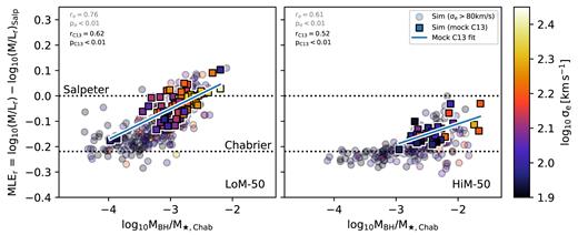
As Fig. 2 but now showing the stellar MLEr as a function of the ratio between MBH and the stellar mass inferred assuming a Chabrier IMF, M⋆,Chab. In both variable IMF simulations, we see a clear trend of increasing MLEr of the stellar population with higher MBH/M⋆,Chab. This result shows that an observed correlation between MLE and MBH/M⋆ does not necessarily imply that MBH is systematically underestimated for high MBH/M⋆,Chab objects. Instead, the trend may be real and a signpost for a variable IMF. The correlations for LoM-50 and HiM-50 come mostly from the fact that galaxies with enhanced MBH/M⋆,Chab tend to originate in higher pressure and older environments, respectively (Barber et al. 2016).
The predicted correlation between MLEr and MBH/M⋆,Chab has important implications for the dynamical measurement of BH masses, especially for recently observed galaxies with puzzlingly overmassive BHs. Both of our IMF prescriptions predict a higher stellar M/L ratio in such galaxies, which must be taken into account when inferring BH masses. Indeed, for our LoM IMF prescription, one would underestimate the stellar mass by a factor of 2 if one assumes a M/L ratio consistent with a Chabrier IMF when converting the K-band luminosity to M⋆, which would result in an overestimation of MBH. Both the underestimate of M⋆ and the overestimate of the MBH serve to artificially increase the ratio MBH/M⋆,Chab. Thus, we suggest that authors who find overmassive BHs in high-mass galaxies consider the possibility that also the IMF may be either top- or bottom-heavy in these systems.
Indeed, one may turn this argument around and suggest that if one were to seek galaxies with non-MW IMFs, a promising place to look is in galaxies with abnormally high MBH/M⋆, such as NGC 1277, NGC 1271 (Walsh et al. 2015), and ultracompact dwarf (UCD) galaxies for which BH mass measurements are available (e.g. M60-UCD1, Seth et al. 2014, although tidal stripping may be responsible for the high BH masses in UCDs; Barber et al. 2016).
4.6 Which observables correlate most strongly with the MLE?
We now determine which of the observable parameters σe, age, [Mg/Fe], metallicity, and re best predict MLEr.5 To do so, we first standardize the logarithm of each parameter such that the mean and dispersion are 0 and 1, respectively, and perform an ordinary linear regression fit to the (standardized) MLEr using all of these parameters simultaneously. We then determine the change in the adjusted coefficient of determination, R2, when each variable is added to the model last, a quantity we will denote as ΔR2. Since R2 gives us the fraction of the variance in MLEr that is explained by the variance in the parameters of the model, ΔR2 gives us insight into the fraction of the variance in MLEr that can be accounted for by the variance in each parameter individually, taking into account the information available through the other input parameters. Note that the sum of ΔR2 values will only equal the total R2 if all of the input variables are completely uncorrelated. For example, two input variables that are strongly correlated will each have ΔR2 ≈ 0, even if individually they can explain much of the scatter in MLEr. Thus, to gain a sense of the contribution of each variable to the total variance in MLEr, we rescale the ΔR2 values such that they sum to R2.
We first perform this analysis on the mock C13 samples, as they should be more directly comparable to galaxy samples in observational IMF studies. The total R2 values (i.e. the fraction of the variance in MLEr that can be explained by all of these parameters) are 0.53 and 0.89 for LoM-50 and HiM-50, respectively. For LoM-50, we find that σe, re, and age are the most important variables, with ΔR2 = 0.20, 0.20, and 0.14, respectively, with much smaller contributions from metallicity and [Mg/Fe]. For HiM-50, [Mg/Fe] is the most important parameter with ΔR2 = 0.45, followed by age (0.34) and metallicity (0.12), with negligible contribution from σe or re. These results are summarized in Table 3.
We conclude that, in a scenario in which the IMF varies at the low-mass end and in such a way as to give the observed trend between MLEr and σe (LoM), then when all other variables are kept fixed we obtain the strongest trend of MLEr with σe, re, and age, with little to no residual dependence on metallicity or [Mg/Fe]. The strong trends with σe, re, and age in our simulations come from the correlation between these parameters and birth ISM pressure, which governs the IMF variations. Indeed, if we include mean light-weighted birth ISM pressure in the fits, the total R2 increases to 0.97, and ΔR2 drops to <0.002 for all of the other input variables, while that for birth ISM pressure is 0.44.6
On the other hand, if the IMF varies at the high-mass end (HiM), we find that the MLEr depends mainly on the age and [Mg/Fe] of the system, with a secondary dependence on metallicity. The strong contribution from [Mg/Fe] comes from the fact that [Mg/Fe] correlates strongly with birth ISM pressure in HiM-50 galaxies, likely due to the enhanced Mg yields resulting from the IMF becoming top-heavier towards higher pressure environments. Indeed, for the HiM-50 simulation, the correlation between [Mg/Fe] and birth ISM pressure is stronger than that between σe and birth ISM pressure, eliminating a need to include σe in the fit to the MLE when [Mg/Fe] is also included. Remarkably, we find that even adding birth ISM pressure to the list of parameters in the above procedures does not add much new information. In this case, total R2 increases from 0.89 to 0.96, with ΔR2 = 0.52 and 0.45 for age and birth ISM pressure, respectively, with negligible contributions from the other input variables. The strong age contribution is due to the dependence of the MLEr on age when the high-mass slope is shallower than the Salpeter value. Indeed, this age dependence would exist even for a non-variable top-heavy IMF. Note as well that a fit to MLEr using only birth ISM pressure as an input variable results in R2 = 0.97 and 0.87 for LoM-50 and HiM-50, respectively (see Table 1). This result highlights the importance of age on the MLEr for high-mass, but not low-mass, IMF slope variations.
Fit parameters to the r-band mass-to-light ratio excess, MLEr, for mock C13 galaxies in our variable IMF simulations. Columns 2 and 3 show the result of a linear least-squares fit of the relation between each parameter (indicated in Column 1) individually and MLEr, of the form MLEr = ax + b. Column 4 shows the coefficient of determination, while columns 5 and 6 show the Spearman-r value and the corresponding p-value.
| x | a | b | R2 | Spearman r | p |
|---|---|---|---|---|---|
| LoM-50 | |||||
| |$\log _{10} P_{\rm birth}/(\, {\rm K}\, {\rm cm}^{-3})$| | 0.12 ± 0.00 | −0.69 ± 0.02 | 0.96 | 0.99 | <0.01 |
| |$\log _{10}\sigma _e/(\, {\rm km}\, {\rm s}^{-1})$| | 0.22 ± 0.05 | −0.52 ± 0.11 | 0.22 | 0.48 | <0.01 |
| log10Age/Gyr | 0.34 ± 0.06 | −0.32 ± 0.05 | 0.32 | 0.61 | <0.01 |
| log10Z/Z⊙ | −0.18 ± 0.08 | 0.01 ± 0.02 | 0.08 | −0.22 | 0.07 |
| [Mg/Fe] | 0.16 ± 0.10 | −0.02 ± 0.01 | 0.04 | 0.21 | 0.09 |
| log10re/kpc | −0.04 ± 0.04 | −0.01 ± 0.02 | 0.02 | −0.06 | 0.65 |
| log10M⋆,Chab | 0.08 ± 0.03 | −0.92 ± 0.29 | 0.12 | 0.38 | <0.01 |
| MK − 5log10h | −0.02 ± 0.01 | −0.53 ± 0.25 | 0.06 | −0.26 | 0.03 |
| log10MBH/M⋆ | 0.11 ± 0.02 | 0.31 ± 0.06 | 0.34 | 0.46 | <0.01 |
| |$\log _{10} \sigma _e^2/r_e\ [{\rm km^2\, s^{-2}\, kpc^{-1}}]$| | 0.15 ± 0.02 | −0.59 ± 0.09 | 0.37 | 0.56 | <0.01 |
| HiM-50 | |||||
| |$\log _{10} P_{\rm birth}/(\, {\rm K}\, {\rm cm}^{-3})$| | 0.07 ± 0.01 | −0.51 ± 0.03 | 0.87 | 0.91 | <0.01 |
| |$\log _{10}\sigma _e/(\, {\rm km}\, {\rm s}^{-1})$| | 0.19 ± 0.08 | −0.52 ± 0.15 | 0.18 | 0.48 | <0.01 |
| log10Age/Gyr | 0.34 ± 0.06 | −0.38 ± 0.04 | 0.53 | 0.68 | <0.01 |
| log10Z/Z⊙ | 0.13 ± 0.06 | −0.22 ± 0.04 | 0.15 | 0.39 | 0.04 |
| [Mg/Fe] | 0.39 ± 0.05 | −0.19 ± 0.01 | 0.72 | 0.81 | <0.01 |
| log10re/kpc | 0.12 ± 0.08 | −0.24 ± 0.06 | 0.09 | 0.24 | 0.21 |
| log10M⋆,Chab | 0.09 ± 0.04 | −1.10 ± 0.40 | 0.17 | 0.36 | 0.06 |
| MK − 5log10h | −0.02 ± 0.02 | −0.66 ± 0.34 | 0.08 | −0.21 | 0.26 |
| log10MBH/M⋆ | −0.01 ± 0.02 | −0.16 ± 0.06 | <0.01 | 0.24 | 0.21 |
| |$\log _{10} \sigma _e^2/r_e\ [{\rm km^2\, s^{-2}\, kpc^{-1}}]$| | 0.08 ± 0.05 | −0.40 ± 0.15 | 0.10 | 0.36 | 0.06 |
For completeness, we repeat this analysis for the full sample of galaxies with |$\sigma _e \gt 10^{1.9}\, {\rm km}\, {\rm s}^{-1}$|, rather than only those that would have been selected by C13. The results are presented in Tables 2 and 4. For LoM-50, we find qualitatively the same conclusions as for the mock C13 sample, except that now re provides much more information than it did for the mock C13 sample (compare Tables 3 and 4), due to the inclusion of compact galaxies with high σe that are too dim to be included in the mock C13 sample. For HiM-50, age, rather than [Mg/Fe], becomes the dominant contributor to the scatter in MLEr due to the inclusion of young galaxies in the σe-complete sample (see Fig. 1). These results highlight the importance of sample selection in determining with which property the IMF correlates most strongly.
As in Table 1 but for all galaxies with |$\sigma _e \gt 10^{1.9}\, {\rm km}\, {\rm s}^{-1}$|.
| x | a | b | R2 | Spearman r | p |
|---|---|---|---|---|---|
| LoM-50 | |||||
| |$\log _{10} P_{\rm birth}/(\, {\rm K}\, {\rm cm}^{-3})$| | 0.12 ± 0.00 | −0.70 ± 0.01 | 0.96 | 0.98 | <0.01 |
| |$\log _{10}\sigma _e/(\, {\rm km}\, {\rm s}^{-1})$| | 0.28 ± 0.03 | −0.68 ± 0.07 | 0.18 | 0.45 | <0.01 |
| log10Age/Gyr | 0.37 ± 0.02 | −0.37 ± 0.02 | 0.46 | 0.72 | <0.01 |
| log10Z/Z⊙ | −0.32 ± 0.03 | 0.00 ± 0.01 | 0.22 | −0.47 | <0.01 |
| [Mg/Fe] | 0.28 ± 0.06 | −0.06 ± 0.01 | 0.07 | 0.21 | <0.01 |
| log10re/kpc | −0.14 ± 0.02 | −0.01 ± 0.01 | 0.17 | −0.39 | <0.01 |
| log10M⋆,Chab | 0.04 ± 0.01 | −0.57 ± 0.15 | 0.03 | 0.14 | 0.01 |
| MK − 5log10h | 0.00 ± 0.01 | −0.03 ± 0.12 | <0.01 | 0.04 | 0.45 |
| log10MBH/M⋆ | 0.13 ± 0.01 | 0.32 ± 0.03 | 0.41 | 0.68 | <0.01 |
| |$\log _{10} \sigma _e^2/r_e\ [{\rm km^2\, s^{-2}\, kpc^{-1}}]$| | 0.20 ± 0.01 | −0.82 ± 0.04 | 0.50 | 0.72 | <0.01 |
| HiM-50 | |||||
| |$\log _{10} P_{\rm birth}/(\, {\rm K}\, {\rm cm}^{-3})$| | 0.05 ± 0.01 | −0.38 ± 0.03 | 0.23 | 0.39 | <0.01 |
| |$\log _{10}\sigma _e/(\, {\rm km}\, {\rm s}^{-1})$| | 0.06 ± 0.04 | −0.28 ± 0.09 | <0.01 | 0.12 | 0.10 |
| log10Age/Gyr | 0.22 ± 0.01 | −0.30 ± 0.01 | 0.68 | 0.87 | <0.01 |
| log10Z/Z⊙ | −0.08 ± 0.02 | −0.12 ± 0.01 | 0.07 | −0.30 | <0.01 |
| [Mg/Fe] | 0.32 ± 0.04 | −0.19 ± 0.00 | 0.27 | 0.36 | <0.01 |
| log10re/kpc | 0.07 ± 0.02 | −0.22 ± 0.02 | 0.03 | 0.28 | <0.01 |
| log10M⋆,Chab | −0.05 ± 0.01 | 0.34 ± 0.13 | 0.07 | −0.24 | <0.01 |
| MK − 5log10h | 0.03 ± 0.00 | 0.42 ± 0.09 | 0.18 | 0.39 | <0.01 |
| log10MBH/M⋆ | 0.05 ± 0.01 | −0.03 ± 0.02 | 0.21 | 0.52 | <0.01 |
| |$\log _{10} \sigma _e^2/r_e\ [{\rm km^2\, s^{-2}\, kpc^{-1}}]$| | −0.02 ± 0.02 | −0.11 ± 0.06 | <0.01 | −0.09 | 0.19 |
Determination of the importance of different observables for predicting MLEr for mock C13 galaxies in our variable IMF simulations. Column 2 gives the fraction of the variance in MLEr that is accounted for by the variance in each variable indicated in Column 1 (see text).
| x | ΔR2 |
|---|---|
| LoM-50 | |
| |$\log _{10}\sigma _e/{\rm (\, {\rm km}\, {\rm s}^{-1})}$| | 0.20 |
| log10Age/Gyr | 0.14 |
| log10Z/Z⊙ | <0.01 |
| [Mg/Fe] | <0.01 |
| log10Re/kpc | 0.20 |
| HiM-50 | |
| |$\log _{10}\sigma _e/{\rm (\, {\rm km}\, {\rm s}^{-1})}$| | <0.01 |
| log10Age/Gyr | 0.34 |
| log10Z/Z⊙ | 0.12 |
| [Mg/Fe] | 0.45 |
| log10Re/kpc | <0.01 |
As in Table 3 but for all galaxies with |$\sigma _e \gt 10^{1.9}\, {\rm km}\, {\rm s}^{-1}$|. Relative to the mock C13 sample, the importance of re and age are enhanced for LoM-50 and HiM-50, respectively, due to in inclusion of dim, compact galaxies with high MLEr in the former, and young, low-MLEr galaxies in the latter.
| x | ΔR2 |
|---|---|
| LoM-50 | |
| |$\log _{10}\sigma _e/{\rm (\, {\rm km}\, {\rm s}^{-1})}$| | 0.22 |
| log10Age/Gyr | 0.16 |
| log10Z/Z⊙ | <0.01 |
| [Mg/Fe] | <0.01 |
| log10Re/kpc | 0.41 |
| HiM-50 | |
| |$\log _{10}\sigma _e/{\rm (\, {\rm km}\, {\rm s}^{-1})}$| | <0.01 |
| log10Age/Gyr | 0.69 |
| log10Z/Z⊙ | 0.06 |
| [Mg/Fe] | 0.16 |
| log10Re/kpc | <0.01 |
Finally, we wish to address the question of whether the MLE correlates more strongly with σe or [Mg/Fe]. Repeating the analysis above for mock C13 galaxies but now only including σe and [Mg/Fe] in the input parameters, we find that for LoM-50, we obtain R2 = 0.19, with ΔR2 = 0.21 and −0.02 for σe and [Mg/Fe], respectively.7 The opposite is true for HiM-50, where we obtain R2 = 0.70, and ΔR2 = −0.01 and 0.71 for σe and [Mg/Fe], respectively. Thus, at fixed σe no correlation exists between MLEr and [Mg/Fe] for low-mass slope variations, while for high-mass slope variations, no correlation exists between MLEr and σe at fixed [Mg/Fe]. These differences are due to the fact that σe correlates more strongly than [Mg/Fe] with birth ISM pressure in LoM-50, but the opposite is true in HiM-50 due to the enhanced Mg yields resulting from a top-heavy IMF in high-pressure environments.
It will be interesting to see on which variables the MLE depends most strongly for observed galaxies, as our results suggest that such relations may be used to break the degeneracy between parametrizations of the IMF. La Barbera et al. (2015) find that the IMF, when parametrized as a top-light ‘bimodal’ IMF, shows no correlation with [Mg/Fe] at fixed σ, which is consistent with our LoM-50 simulation. It would be interesting to know if this is still true when parametrizing the IMF with low-mass slope variations instead (as in LoM). Indeed, Conroy & van Dokkum (2012) find that the IMF correlates more strongly with [Mg/Fe] than with σ when varying the low-mass slope of the IMF. However, comparisons between IMF studies are difficult due to differences in apertures, methods, and IMF parametrizations employed. We encourage spectroscopic IMF studies to test different parametrizations of the IMF to assess the robustness of correlations between the IMF and galaxy properties, which can then be compared with the predictions presented here. Note that this does not apply to studies that measure the MLE dynamically, as no assumption of IMF parametrization is needed.
5 MLE OF SATELLITE GALAXIES
We also briefly investigate the effect of environment on the IMF, where in Fig. 6 we show the MLEr−σe relation at |$z$| = 0.1 for the two variable IMF simulations split into central and satellite galaxies. Central galaxies are defined for each FoF group as the subhalo to which the most bound gas particle of the group is bound, while all other subhaloes within the group are satellites. For both simulations, on average there is little difference between the two populations, given their significant overlap at fixed σe. However, some satellites tend to scatter towards highigher MLEr values than centrals, especially for |$\sigma _e \lt 100\, {\rm km}\, {\rm s}^{-1}$|. This effect is stronger in LoM-50 (although it is still visible in HiM-50), resulting in a median MLEr for satellites that is larger by |${\approx } 0.05\, {\rm dex}$| at |$\sigma \approx 100 \, {\rm km}\, {\rm s}^{-1}$|. These outliers are likely the stellar cores left over from tidal stripping events. This result can be understood in the context of radial IMF variations, where the central, more tightly bound stars, being born at higher pressures than those in the outer regions, have heavier IMFs than the outer regions that have since been stripped. Indeed, we will show in Paper III that such radial IMF gradients are stronger in LoM-50 galaxies than in HiM-50.
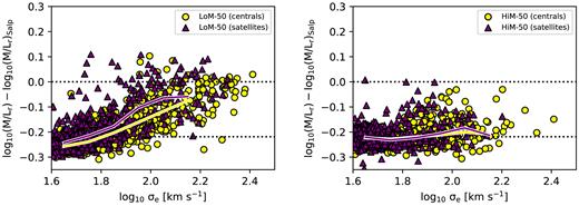
Excess M/Lr ratio relative to a Salpeter IMF as a function of the central stellar velocity dispersion, σe, separated into central (yellow circles) and satellite (purple triangles) galaxies at |$z$| = 0.1. The left-hand and right-hand panels show galaxies from LoM-50 and HiM-50, respectively. All quantities are measured within the 2D projected stellar r-band half-light radius. The solid lines indicate running medians of bin size 0.1 dex in σe. Satellites generally follow the same trend as centrals, but lower-σe satellites scatter towards higher MLEr than centrals due to tidal stripping leaving only the IMF-heavy, inner regions bound to the subhalo.
This result has important consequences for the inference of the stellar mass of satellite galaxies, where, for these variable IMF prescriptions, the underestimate of the inferred stellar masses (assuming a Chabrier IMF) may be as high as a factor of 2 if they have been significantly stripped. Indeed, recent studies (e.g. Mieske et al. 2013; Seth et al. 2014; Villaume et al. 2017) find elevated dynamical M/L ratios in UCDs, and have argued for one of two scenarios: either i) these UCDs are the remnant cores of tidally stripped progenitor galaxies and the extra mass comes from a now overmassive central BH, or ii) the IMF in these galaxies is top- or bottom-heavy. Our results show that both cases can be expected to occur simultaneously, as tidal stripping will increase both MLEr, as the ‘IMF-lighter’ outskirts are stripped, as well as MBH/M⋆, as the galaxy loses stellar mass.
These results are possibly at odds with the recent work of Rosani et al. (2018), who found no environmental dependence of the IMF in the σe-stacked spectra of ETGs from SDSS. However, such an analysis would miss outliers due to the σe-stacking. Better statistics at the high-mass end would be required for a more in-depth comparison with their work.
6 SUMMARY AND CONCLUSIONS
We use cosmological, hydrodynamical simulations with self-consistent variable IMF prescriptions to investigate trends between the MLE relative to that expected for a Salpeter IMF and global galaxy properties such as age, metallicity, and alpha abundance. These simulations follow the EAGLE reference model (Schaye et al. 2015) except that the IMF becomes either bottom-heavy (the LoM-50 simulation) or top-heavy (HiM-50) for individual star particles formed in high-pressure (or, equivalently, high-SFR surface density) environments. These simulations are unique in that the IMF variations have been calibrated to match the observed trend of increasing MLE with central stellar velocity dispersion, σe (Cappellari et al. 2013b, hereafter C13). This calibration is possible due to the fact that stars in the centres of ETGs form at higher pressure with increasing σe. The MLE increases with σe due to an increased fraction of low-mass stars in LoM-50, and an increasing mass fraction of stellar remnants and decreased luminosity in HiM-50. We verified in Paper I that the variable IMF simulations reproduce the observables used to calibrate the EAGLE subgrid models for feedback: the galaxy luminosity function, half-light radii, and BH masses. The goal of this paper is to determine the similarities and differences in the relationships between the MLE and global galaxy properties that are expected to result from a galaxy formation model with self-consistent, calibrated IMF variations, in order to help interpret such relationships for observed galaxies and distinguish between different IMF variation scenarios.
Our conclusions are as follows:
The MLE is only a good indicator of IMF slope, independent of age or metallicity, if the high-mass slope is kept fixed at the ‘reference’ value (in our case Salpeter). If the high-mass slope is varied, as is the case for HiM-50, the MLE becomes as sensitive to age as it is to the IMF (Fig. 1).
Trends of MLE with overall galactic properties were investigated for properties measured within the half-light radius, re, for galaxies selected in a way similar to the sample of C13 from ATLAS3D (Fig. 2). For LoM-50, MLE correlates positively with age and [Mg/Fe], and negatively with metallicity. However, the significance of the correlations of MLE with metallicity or [Mg/Fe] depends on galaxy selection effects. The anticorrelation with metallicity is the result of the decreasing Z with σe at high σe and the tight MLE−σe relation in that simulation. For HiM-50, MLE also correlates positively with age and [Mg/Fe] but has no significant correlation with metallicity due to the fact that the C13 selection criteria exclude faint, old, low-metallicity galaxies with high MLE that would otherwise help drive a negative trend in a σe-complete sample. Fits are shown in Fig. 2 and Table 1. We will show in a companion paper that the spatially resolved versions of these relations (i.e. trends within galaxies) differ qualitatively from the global trends presented here.
For both LoM-50 and HiM-50, the MLE correlates positively with mass and luminosity, but with more scatter than the MLE−σe trend (Fig. 3). For LoM-50, MLE anticorrelates with half-light radius, re, at fixed σe due to the fact that smaller high-σe galaxies form stars at higher pressures. This anticorrelation is, however, sensitive to observational selection effects that may prefer larger systems. MLE correlates positively with re for HiM-50 due to a lack of small high-σe galaxies, which tightens the positive relation between re and σe in the HiM-50 simulation (Fig. 4). These differences can be explained by the weaker (stronger) stellar feedback in high-pressure environments in LoM-50 (HiM-50) that can decrease (increase) galaxy sizes.
A luminosity-complete sample of old, early-type galaxies, as is used in Cappellari et al. (2013b), exhibits significant biases in the correlations between the MLE and global galaxy properties such as metallicity, stellar mass, luminosity, and size relative to a galaxy sample that is complete in σe (Figs 2 and 3). Care must thus be taken by observational studies to ensure that selections on properties such as morphology, age, or luminosity do not affect the inferred relations.
Of the variables σe, age, metallicity, [Mg/Fe], and re, we determined the importance of each variable in explaining the variance in the MLE. For LoM-50, σe, re, and age account for the most variance in MLE, while the contributions from metallicity and [Mg/Fe] are much smaller. This result reflects the correlations of birth ISM pressure with σe, re, and age, and the weak effect that low-mass slope variations have on abundances. For HiM-50, [Mg/Fe] and age are the largest contributors to the variance in the MLE, with a smaller but significant contribution from metallicity, and negligible contributions from σe and re. This strong age-dependence is due to the sensitivity of the MLE on age for a top-heavy IMF, rather than to any age dependence of the IMF itself. The dependence on abundances likely arises due to the impact of the top-heavy IMF on the stellar yields (see Table 3).
MLE correlates quite strongly with MBH/M⋆,Chab for both variable IMF simulations (Fig. 5). This finding suggests that in the variable IMF scenario, galaxies with BHs that are bona fide overmassive relative to the MBH−M⋆ relation should also have ‘heavy’ IMFs. This correlation likely results from the fact that older galaxies tend to form their stars and BHs at higher pressures, leading to both overmassive BHs (Barber et al. 2016) and heavy IMFs. We conclude that even though a degeneracy in principle exists between the dynamical calculation of MBH and stellar M/L ratio in observed galaxies, a correlation between MBH/M⋆,Chab and MLE does not imply that overmassive BHs are necessarily the result of incorrect IMF assumptions, nor that excess M/L ratios are solely the result of overmassive BHs.
Satellite galaxies mainly follow the same MLE−σe trend as central galaxies, with a few per cent scattering towards high MLE due to tidal stripping removing the outer ‘light IMF’ regions, leaving only the ‘heavy IMF’ core prior to being completely destroyed by tidal forces. This effect is stronger for LoM-50 than for HiM-50 (Fig. 6).
Overall, we have found that an IMF that varies with the local physical conditions, in our case birth ISM pressure, yields a galaxy population for which the MLE correlates with many global galaxy properties. Interestingly, if the high-mass end of the IMF varies, then some correlations can be as strong or stronger than the correlation with birth pressure due to the strong dependence of MLE on age. Our two IMF prescriptions yield qualitatively similar correlations between the MLE and global galaxy properties, particularly with age and [Mg/Fe]. The difference between their predicted correlations with re as well as that between the importance of different parameters in predicting the MLE can be used to differentiate between these two IMF variation scenarios. In Paper III, we will investigate further the predicted differences between these simulations by probing the spatially resolved inner regions of high-mass galaxies to uncover the local behaviour of IMF variations and their impact on, and scaling with, other spatially resolved properties. Paper III will additionally investigate the effect of these IMF variations on the evolution of galaxies in the simulations.
ACKNOWLEDGEMENTS
We are grateful to the anonymous referee for helping to improve the quality of the paper. This work used the Distributed Research utilizing Advanced Computing (DiRAC) Data Centric system at Durham University, operated by the Institute for Computational Cosmology on behalf of the Science & Technology Facilities Councel (STFC) DiRAC High Performance Computing Facility (www.dirac.ac.uk). This equipment was funded by the Department for Business Innovation & Skills (BIS) National E-infrastructure capital grant ST/K00042X/1, STFC capital grants ST/H008519/1 and ST/K00087X/1, STFC DiRAC Operations grant ST/K003267/1, and Durham University. DiRAC is part of the National E-Infrastructure. RAC is a Royal Society University Research Fellows. We also gratefully acknowledge the Partnership for Advanced Computing in Europe (PRACE) for awarding us access to the resource Curie based in France at Très Grand Centre de Calcul. This work was sponsored by the Dutch National Computing Facilities Foundation (NCF) for the use of supercomputer facilities, with financial support from the Netherlands Organization for Scientific Research (NWO). This research used astropy, a community-developed core python package for Astronomy (Astropy Collaboration 2013).
Footnotes
Note that the trend flattens at the Kroupa value for high-mass slopes steeper than −2.1, and the trend would actually reverse if the high-mass slope were to become steeper than Salpeter (<−2.35).
Also note that Conroy & van Dokkum (2012) measure dynamical M/L within re but spectroscopic M/L within re/8.
Solar abundances for Mg and Fe are taken from Asplund et al. (2009).
Note that in this analysis we leave out mass and luminosity because these are used to compute MLE in the first place, so correlations between them and the MLE would not be as meaningful.
Note that R2 is not exactly 1.0 even when correlating MLE with birth ISM pressure directly, due to the fact that the MLE is averaged over many star particles with a potentially wide range of M/L ratios, and that the MLE is not a perfect measure of the IMF even for individual star particles due to some age and metallicity dependence.
Note that since we use the adjusted R2, it is possible to have slightly negative ΔR2 for some variables due to the penalty for adding extra data with no extra information.
