


ABSTRACT
R Coronae Borealis (RCB) stars are predominantly metal-poor, near-solar mass hydrogen-deficient carbon-rich supergiants that have evolved from mergers of carbon–oxygen and helium white dwarf (WD) systems. They have some of the lowest 16O/18O ratios measured in any star (between 1 and 25) and are also enhanced compared to solar, in fluorine and the s-process elements. In the paper by Menon et al., post-WD-merger stellar evolution models of RCBs constructed at solar metallicity could reproduce the above chemical signatures. In this work, we construct new post-WD-merger models with a realistic RCB metallicity of [Fe/H] = −1.4, using the same methodology as Menon et al. An important aspect of this method was the inclusion of an artificial mixing process during the evolution of the models, which was essential to reproduce the isotopic ratios of RCBs. The surface of our new post-merger models have 16O/18O ratios of 9.5–30, 12C/13C ratios of 1500–7000 which overlap with the values recorded for RCBs, along with their enhancements in fluorine and in s-process elements. We then explore the possibility that a fraction of pre-solar low-density graphite grains, those with comparable 16O/18O and 12C/13C ratios as RCBs, were formed in the outflows of these stars. On assuming that the gas ejected by RCBs would have mixed with its surrounding interstellar material of solar composition, our models can reproduce some of the isotopic ratios of these graphite grains, thereby strengthening the hypothesis that RCB stars could be a source of some pre-solar graphite grains.
1 INTRODUCTION
R Coronae Borealis stars (RCBs) are carbon-rich supergiants that are almost entirely deficient in hydrogen (Searle 1961; Pollard, Cottrell & Lawson 1994; Asplund et al. 1997, 2000). RCBs have been found in the Magellanic Clouds and in the old bulge population of our Galaxy (Cottrell & Lawson 1998; Alcock et al. 2001; Tisserand et al. 2008; Clayton 2012; Tisserand et al. 2013) and recently also in the Andromeda galaxy (Tang et al. 2013). The Galactic population of RCBs have metallicities of [Fe/H]<−0.6, with the majority of these have effective temperatures of |$3000\, \mathrm{K}\le T_\mathrm{eff}\le 8000\, \mathrm{K}$| and luminosities of |$3.5\le \mathrm{log}\, L/\mathrm{L}_{\odot}\le 4.0$| (Clayton 1996; Asplund et al. 2000; Pandey, Lambert & Kameswara Rao 2008). Four RCBs have also been discovered with |$T_\mathrm{eff}=15\, 000\text{-}25\, 000$| K (Alcock et al. 2001; Clayton 1996, 2012).
RCBs were first noted for their distinct light curves which underwent unpredictable declines in brightness of up to eight orders of magnitude (Loreta 1935; O’Keefe 1939; Feast et al. 1997; Feast 1997). These declines were attributed to puffs of amorphous carbon dust released from the atmosphere of the star (Feast 1986; Clayton 1996; García-Hernández, Rao & Lambert 2011), whose ejections coincided with the pulsation period of the star (Woitke, Goeres & Sedlmayr 1996; Crause, Lawson & Henden 2007; Lawson et al. 1990). Typically each puff of carbon dust has a mass of |$10^{-6}\text{-}10^{-7}\, \mathrm{M}_{\odot} \,$| (Feast 1986; Clayton et al. 2011).
The atmospheres of RCBs have many chemically peculiar signatures, the most remarkable of them being some of the lowest 16O/18O number ratios detected in any star, between 1 and 25 as against the solar value of ∼500 (Clayton et al. 2007; García-Hernández et al. 2010). They also have high 12C/13C number ratios >40–100 (Warner 1967; Cottrell & Lambert 1982; Hema, Pandey & Lambert 2012), with the exception of a few stars with 12C/13C = 3–4 (Rao & Lambert 2008; Hema et al. 2012), along with enhancements in F of up to 2.7 dex (Pandey et al. 2008) and in s-process elements (Asplund et al. 2000) compared to solar. Two evolutionary channels have been proposed to explain the origin of RCBs. In the final flash (FF) scenario, a post-AGB star that is transitioning to the white dwarf (WD) cooling track after mass loss has removed most of its envelope, undergoes a late He-shell flash and loops back to the AGB (Renzini 1990). In the alternative scenario, a binary system of degenerate carbon–oxygen (CO) and helium (He) WDs merge over the dynamical timescale and the post-merger structure is expected to relax and attain thermal equilibrium as a supergiant. This is called the double degenerate (DD) scenario (Webbink 1984; Iben, Tutukov & Yungelson 1996).
Two observational deductions favour the DD scenario over the FF scenario. FF models have He-burning temperatures that can completely destroy the 18O and 19F to 22Ne (Clayton et al. 2007; Werner & Herwig 2006; Herwig et al. 2011), while high amounts of 18O and 19F have been detected in the atmosphere of RCBs. Stars originating from an FF scenario, such as Sakurai’s object, have a low 12C/13C ratio of ∼1.5–5 (Asplund et al. 1997), whereas most RCBs have higher values of >40. The second reason in favour of the DD scenario is the estimated mass of RCBs of |$0.8\text{-}0.9\, \mathrm{M}_{\odot},$| which were inferred from their pulsation periods (Saio 2008). As the star undergoing the late He-shell flash in the FF scenario has a CO WD and a thin envelope, its mass would be close to typical CO WD masses, of |$0.5\text{-}0.7\, \mathrm{M}_{\odot} \,$| (Bergeron, Gianninas & Boudreault 2007; Tremblay et al. 2016), which is less than the measured mass of RCBs. Since the DD scenario involves an He and a CO WD, the mass of the star arising from their merger can be within the observationally estimated value.
Overall, the DD evolutionary channel appears to be the main channel of formation for RCBs and have been studied by a number of authors such as Saio & Jeffery (2002), Clayton et al. (2007), Lorén-Aguilar, Isern & García-Berro (2009), Jeffery, Karakas & Saio (2011), Longland et al. (2011), Staff et al. (2012), Menon et al. (2013), and Zhang et al. (2014). The duration of the RCB phase is not well constrained and is expected to be of the order of 104–105yr from observations (Clayton et al. 2011; Clayton 2012). The post-merger models of Menon et al. (2013) had a lifetime of 0.97–2.75 × 10⁵ yr as RCBs.
1.1 Evolutionary models for RCBs
A DD WD system is formed from an initial setup that consists of a pair of main-sequence intermediate-mass stars. Two common envelope episodes occur during their evolution– one when the more massive star (primary) evolves into an asymptotic giant branch (AGB) star with a degenerate CO core and another when the secondary evolves into a red giant branch (RGB) star with a degenerate He core (Webbink 1984; Iben et al. 1996; Solheim 2010; Brown et al. 2016). In the second common envelope phase, the entire envelope is ejected and results in a close CO + He WD binary with an orbital period of a few hours. A number of such close DD systems have been found by many observational surveys (e.g. Nelemans et al. 2005; Schreiber et al. 2009).
Further evolution of the DD system is driven by gravitational wave radiation and magnetic wind braking, which further shrink the orbital separation. The next phase of the binary system is expected to be the merger of the WDs. Mergers have been modelled in 3D hydrodynamic simulations such as those by Benz et al. (1990), Segretain, Chabrier & Mochkovitch (1997), Lorén-Aguilar et al. (2009), Dan et al. (2011), Raskin et al. (2012), Staff et al. (2012), Dan et al. (2014), and Moll et al. (2014). The He WD was found to be tidally disrupted by the more massive CO WD, with a stream of the He WD mass rapidly falling on the CO WD thereby creating a hot corona like structure around the CO WD, while the majority of the unbound He WD settled as a cold disc. The complete disruption of the He WD, the dynamic merger phase, lasted for a period of a few minutes in these simulations.
The next phase is the long-term evolution of the post-merger object. Shen et al. (2012) and Schwab et al. (2012) found that magnetic stresses redistribute angular momentum through the envelope of the post-merger object and over a period of 104–108 s, the differentially rotating post-merger remnant evolves to a spherically symmetric structure with a thermally supported envelope in solid-body rotation. Both papers predict that after the viscous phase, the structure can evolve over a thermal time-scale into a giant star with an extended envelope driven by convection. Zhang et al. (2014) built zero-metallicity 1D models of the ‘corona + disc’ structure indicated in the 3D merger simulations. These post-merger models passed through the RCB region in the HR diagram and were also enriched in C, N, O, and F in the surface due to convection driven by He-shell flashes, during the accretion of the disc on the corona.
Menon et al. (2013) also studied the long-term evolution of the WD merger remnant with the aim of obtaining the surface composition of RCBs and their position in the HR diagram. They constructed a 1D hybrid CO + He WD structure by mapping the chemical composition of solar metallicity CO and He WDs onto an initially homogeneous 0.90|$\, \mathrm{M}_{\odot}$| pre-main-sequence model. The temperature–density profile and isotopic abundances of the hot corona from the 3D simulations of Staff et al. (2012), which the authors had named the ‘Shell of Fire’ (SOF), were mapped onto the hybrid structure as well. These post-merger models were then evolved until they passed through the RCB domain in the HR diagram.
During the post-merger evolution, it was observed that there was very little mixing occurring in the model except for a thin convective layer (|$\lt\! 0.01\, \mathrm{M}_{\odot} \,$|) in the surface. The nuclear products that enrich the surface of RCBs were being formed in the interior of the model and there was no mechanism to dredge them up to the surface. Given that the envelope of the post-merger remnant is expected to evolve toward solid-body rotation (Shen et al. 2012; Schwab et al. 2012), mixing processes other than convection can arise due to rotational instabilities. The main isotopic signature that Menon et al. (2013) aimed to reproduce was the low 16O/18O ratio observed in RCBs. Given that the exact nature of rotation-driven mixing processes and their physics are highly uncertain, Menon et al. (2013) constructed an adhoc mixing recipe in the form of an Eulerian diffusion coefficient that would help dredge up sufficient amounts of 12C and 18O to the surface. With this induced mixing, the post-merger models were not only successful at reproducing 16O/18O ratios of 9–15 and 12C/13C > 100, they could also obtain enhancements in F of 1.4–2.35 dex compared to solar, enhancements in s-process elements and reasonably reproduce the abundances of other species observed in RCBs. The mixing routine and its parameter values were set at the initial point of evolution of the model and not altered at any time during the evolution or on an element-by-element basis. This indicates a fair robustness in the mixing prescription and may provide an insight into the kind of mixing that could occur in the long-term evolution of post-DD merger objects.
1.2 Pre-solar graphite grains and their sources
Pre-solar carbon grains are found in three forms: diamonds, silicon carbide grains, and the rarest of the three, graphites (Zinner 2014). Graphites are classified morphologically into two categories based on their density– high-density (HD) and low-density (LD) graphite grains. A subset of graphite grains have low16O/18O ratios ≤ 25 and 12C/13C > 40 (Amari et al. 1993), which are comparable to the values measured in RCBs– these grains belong to the LD class of graphite grains and is the sample set we will use in this study. LD graphite grains generally contain low 29Si/28Si and 30Si/28Si ratios, low 14N/15N ratios, high 26Al/27Al ratios, and excesses in Ca and Ti isotopic ratios compared to their respective solar values (Amari, Zinner & Lewis 1995; Amari & Lodders 2007). Some grains also have 44Ca detected in them, which would have formed from the decay of 44Ti.
1.2.1 Dust from Type II supernovae
Carbon dust grains have been detected in the spectra of ejecta surrounding the remnants of Type II-Plateau supernovae (Type II-P SNe) such as those of SN 1987A, Crab Nebula, and Cas A (Matsuura et al. 2011, 2015; Barlow et al. 2010; Arendt et al. 2014; Gomez et al. 2012; Temim & Dwek 2013). Additionally, the high Ca and Ti isotopic ratios measured in pre-solar graphite grains, their low 29Si/28Si and 30Si/28Si ratios that are interpreted as an excess in 28Si, along with the presence of 44Ca which form from the decay of 44Ti, indicate that these grains may have originated from the explosions of massive stars as Type II-P SNe (Zinner 2014). The subset of grains we are interested in do not have any 44Ca detected in them but they do have low ratios of 29Si/28Si and 30Si/28Si and high ratios of 26Al/27Al, compared to solar.
Typically hence, progenitors of Type II-P SNe have been studied as a source of all graphite grains (Travaglio et al. 1999; Pignatari et al. 2013; Amari, Zinner & Gallino 2014; Pignatari et al. 2015). Since oxygen is more abundant than carbon in the ejecta of Type II-P SNe, the models of Travaglio et al. (1999), Yoshida, Umeda & Nomoto (2005), and Yoshida (2007) preferentially mixed the C-rich layer of the ejecta while avoiding contamination with the O-rich layers in between, to obtain a layer with C/O > 1 in which carbon grains can form. These authors then compared the isotopic ratios of this layer with those of pre-solar graphite grains and obtained varying degrees of success in reproducing them. In a different model, Pignatari et al. (2013, 2015) demonstrated that a C-rich layer in the ejecta can be formed without any preferential mixing, by ensuring the availability of He or H nuclei in the He/C and C/O regions prior to the arrival of the supernova shockwave. On comparing the abundances from explosive He burning due to the passage of the shockwave in these C-rich shells, the authors could obtain many of the isotopic ratios measured in the grains.
1.2.2 Dust from RCBs
Given that the circumstellar environment of an RCB star is rich in carbon dust, RCBs may also be a potential source for pre-solar graphite grains. The current observed number of RCBs including those found in the Galaxy and the Magellanic Clouds, is close to 100 (Clayton 1996; Alcock et al. 2001; Tisserand et al. 2008, 2013). Assuming WD mergers are the channel for their formation and given a merger rate of |$1.8 \times 10^{-2}\, \mathrm{yr}^{-1}$| for CO + He WD systems (Han 1998), Clayton (2012) estimated that 5400–5700 RCBs must currently exist in our Galaxy. They also arrived at a similar number using an independent method that extrapolated the known RCB population in the Large Magellanic Cloud to that of our Galaxy. Karakas, Ruiter & Hampel (2015) estimated a more conservative number of 150–540 RCBs in the Galaxy, based on a lower CO + He WD merger rate of |$1.8 \times 10^{-3}\, \mathrm{yr}^{-1}$|. RCBs are expected to eject about |$10^{-6}\, \mathrm{M}_{\odot} \, \mathrm{yr}^{-1}$| (Feast 1986) to |$10^{-7}\, \mathrm{M}_{\odot} \, \mathrm{yr}^{-1}$| (Clayton et al. 2011) and have a lifetime of roughly 105 yr (Clayton et al. 2011; Clayton 2012). Thus, an RCB star can eject |$0.01\text{-}0.1\, \mathrm{M}_{\odot} \,$| of amorphous carbon dust over its lifetime. With these numbers, Karakas et al. (2015) concluded that the dust production rates of RCBs in the Galaxy may exceed those of born-again AGB stars and novae, and hence could be viable producers of cosmic dust.
Since some LD graphite grains had 16O/18O ≤ 25 and 12C/13C > 40 detected in them (and no 44Ca), Karakas et al. (2015) hypothesized that these pre-solar grains may have originated in the circumstellar environment of RCBs. In particular, since Menon et al. (2013) had conducted a detailed element-by-element comparison between their RCB models and the observed values, Karakas et al. (2015) speculated whether these models could reproduce the isotopic ratios measured in the above subset of LD graphite grains. Although typically the sources of pre-solar grains are considered to be of solar metallicity, the RCBs recorded so far are metal poor, i.e. their [Fe/H] ratios are <−0.6 (Asplund et al. 2000; Pandey et al. 2008; Jeffery et al. 2011). This means the generation of RCBs that were present 4.5 Gyr ago were also metal-poor and their ejected dust could have mixed with the interstellar medium from which the solar system formed. Hence, it is reasonable to study these stars as sources of pre-solar grains.
1.3 Aims of this work
In this work, we build post-merger models with an alpha-enhanced initial composition at a realistic RCB metallicity of Z = 0.0028 ([Fe/H] = −1.4), using the same methodology as Menon et al. (2013, hereby Paper I). The models are evolved through the RCB phase in the HR diagram, during which we examine if their surfaces can reproduce the isotopic ratios of RCBs. We also make detailed comparisons with all the elemental abundances measured in RCBs. We then explore how well the isotopic ratios from these models compare with those LD graphite grains that have 16O/18O and 12C/13C ratios in the observed range of RCBs. In Section 2, we describe the methodology of our work; in Section 3, we present the result of our comparison study and in Section 4, we present our conclusions and discuss their implications.
2 METHODOLOGY
We describe the setup of our initial post-merger models and the artificial mixing recipe. We then vary the initial parameters and build four cases to study in this paper.
2.1 Initial setup
The initial model for the evolutionary calculations consists of four zones which were identified in the hydrodynamic simulations of CO + He WD mergers by Staff et al. (2012): the CO core, the buffer, the SOF, and the envelope (Fig. 1). Material was dredged up during the merger in the simulations from the region between the CO core and the surface of the CO WD and mixed with the overlying He WD material; most of the dredged-up mass was found in the hot SOF region, while the rest was in the envelope.
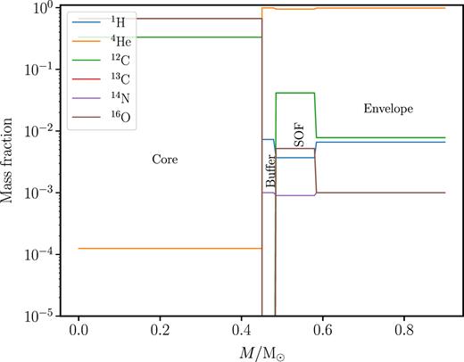
The four-zone profile of the initial post-merger model of Case 1 of this paper.
Our four cases are built using the initial mass distribution of Case 1 of Paper I, which had the lowest surface 16O/18O ratio for its RCB model in that work. The initial WD masses for this case are: |$M_\mathrm{CO\, WD}=0.53$||$\, \mathrm{M}_{\odot}$|, |$M_\mathrm{He\, WD}=0.37$||$\, \mathrm{M}_{\odot}$|, and thus have a total mass of |$M_\mathrm{total}=0.90\, \mathrm{M}_{\odot} \,$|. We refer the reader to Section 2.1.1 of Paper I for a detailed explanation of the construction of the four zones of the initial model. We provide a brief overview of the four zones here:
Core(0.45|$\, \mathrm{M}_{\odot}$|): CO core of the CO WD. This part does not participate in the evolution of the post-merger star.
Buffer(0.03|$\, \mathrm{M}_{\odot}$|): a small buffer zone with the abundances of the He WD.
SOF(0.10|$\, \mathrm{M}_{\odot}$|): a hot shell with temperatures of TSOF = 120–250 MK and densities of ρSOF ≈ 3–5 × 10⁴ g cm−3, suitable for H burning and partial He burning. 50 per cent of the composition is of the dredged up mass from the CO WD and 50 per cent is the He WD composition.
Envelope (0.32|$\, \mathrm{M}_{\odot}$|): relatively cold material where 90.6 per cent of the composition is of the He WD material and 9.4 per cent is that of the dredged-up mass from the CO WD .
After the allotment of masses for the individual zones, the next step is to determine the initial composition of each zone in the model. For this, we first consider the abundances for the CO and He WDs. The abundances of the He WD are extracted from an RGB model of a 1|$\, \mathrm{M}_{\odot}$| main-sequence star, which has an |$M_\mathrm{He\, WD}=0.30\, \mathrm{M}_{\odot} \,$|. Since in the hydrodynamic simulations, the entire He WD was found to be disrupted during the merger we assume a uniform composition for the He WD mass. This composition is then normalized to the He WD mass of |$M_\mathrm{He\, WD}=0.37$||$\, \mathrm{M}_{\odot}$| which was used for the merger simulation. The abundances of the CO WD are taken from an early-AGB model of a 3|$\, \mathrm{M}_{\odot}$| main-sequence star, which has a CO WD mass of |$M_\mathrm{CO\, WD}=0.70\, \mathrm{M}_{\odot} \,$|. We dredge-up |${\sim }35{{\ \rm per\ cent}}$| of the CO WD mass, which includes the envelope and the He shell just above the CO core, which was the same region dredged up to construct models in Paper I as well. The abundances in the dredged up region are homogenized over the dredged up mass of 0.245|$\, \mathrm{M}_{\odot}$| and mixed in required proportions in the SOF and the envelope above it to build the initial composition profile of the model. This initial composition (Fig. 1) is then relaxed on an |$M=0.90\, \mathrm{M}_{\odot} \,$| pre-main-sequence star. Table 1 lists the CO and He WD abundances used in this work. The abundances of the SOF are treated specially, which we shall discuss in the next section.
Isotopic mass fractions from the He WD models (limited to values >10−4) with different envelope masses: He WD(1): |$M_\mathrm{env}=6.4\times 10^{-3}\, \mathrm{M}_{\odot} \,$|, He WD(2): |$M_\mathrm{env}=10^{-2}\, \mathrm{M}_{\odot} \,$| and from the dredged-up region of the CO WD: CO WD (DUP).
| Species | He WD(1) | He WD(2) | CO WD (DUP) |
|---|---|---|---|
| 1H | 7.3 × 10⁻³ | 1.4 × 10⁻² | – |
| 4He | 0.99 | 0.98 | 0.91 |
| 12C | – | – | 8.3 × 10⁻² |
| 13C | – | – | – |
| 14N | 1.0 × 10⁻³ | 1.0 × 10⁻³ | 8.0 × 10⁻⁴ |
| 16O | – | – | 1.0 × 10⁻² |
| 18O | – | – | – |
| Species | He WD(1) | He WD(2) | CO WD (DUP) |
|---|---|---|---|
| 1H | 7.3 × 10⁻³ | 1.4 × 10⁻² | – |
| 4He | 0.99 | 0.98 | 0.91 |
| 12C | – | – | 8.3 × 10⁻² |
| 13C | – | – | – |
| 14N | 1.0 × 10⁻³ | 1.0 × 10⁻³ | 8.0 × 10⁻⁴ |
| 16O | – | – | 1.0 × 10⁻² |
| 18O | – | – | – |
The RGB and AGB star models, from which the He WD and CO WD abundances were extracted respectively, were computed with the stellar evolution and nucleosynthesis post-processing codes used in Karakas, Marino & Nataf (2014) and Karakas & Lugaro (2016). These models were built with an initial composition by setting a global metallicity of Z = 0.0028, where Z = Zα + Zother, where Zother = ZCNO + ZFe, etc. The inferred [Fe/H] value for this metallicity is −1.4. The α-elements are individually enhanced according to the chemical evolution models of Kobayashi, Karakas & Umeda (2011), while the non-α elements are scaled according to the solar abundances and isotopic ratios in Asplund et al. (2009).
Finally, we set up the artificial mixing routine. Menon et al. (2013) adopted an empirical mixing law in the form of an Eulerian diffusion coefficient that drops exponentially from the surface until a cut-off point in the interior of the model. The total diffusion coefficient of the mixing model is the sum of the diffusion coefficient of convective mixing (which is only present within |$\lt\! 0.01\, \mathrm{M}_{\odot} \,$| of the surface) and that of the additional mixing we implement. Mixing is restricted to occur only in the region between the surface and the outer boundary of the CO core (at 0.45|$\, \mathrm{M}_{\odot}$| in our models), i.e. the CO core does not participate in determining the abundances of the surface. Mixing further into the CO core would cause a dredge-up of 16O that would excessively exceed the abundance of 18O in the surface. The additional diffusion coefficient is built such that it drops exponentially from the surface to the location of the entropy barrier arising from the energy peak of nuclear burning, which is approximated as the mass coordinate where the 14N abundance drops to a specific fraction. For more details about the mixing routine, we encourage the reader to refer to Section 2.3 of Paper I. In this work, we use the same parameter values for the additional mixing diffusion coefficient as in Paper I.
2.2 The four cases of this paper
During the initial examination of the models, two important factors were found to affect the surface abundances of the models– the H-rich envelope mass of the He WD and, the SOF. The four cases we study are built so as to isolate the impact of these factors on the post-merger model.
The H-rich envelope masses for the WDs are a function of their H-free core mass (Schoenberner 1983; Driebe et al. 1998) and are found to decrease as the H-free core mass increases. The envelope mass is obtained from a linear fit to models by Staff et al. (2012): |$\mathrm{log}\, M_\mathrm{env}/\mathrm{M}_{\odot}=-4.982\, M_\mathrm{H}/\mathrm{M}_{\odot} - 0.7171$|, where MH is the mass of the H-free core. The CO and He WD masses obtained from the AGB and RGB models are 0.7 and 0.3|$\, \mathrm{M}_{\odot}$| , respectively. Hence with this equation, the envelope masses for the CO and He WD are 4.4 × 10⁻⁴ and |$8.6\times 10^{-4}\, \mathrm{M}_{\odot} \,$| respectively. On running a simulation with these envelope masses, we do not find the required low 16O/18O ratio in the models. We hence increase the envelope mass of the He WD to |$6.4\times 10^{-3}-10^{-2}\, \mathrm{M}_{\odot} \,$|. The fact that the surface abundances are sensitive to the initial H mass was also found in Paper I. The abundances from the two He WD models with differing envelope masses are listed in Table 1.
With a given envelope mass for the He WD, we next construct the SOF abundances. In the hydrodynamic simulations, the SOF is the hottest region during the merger, reaching temperatures of |$123\text{-}250\,$|MK, and hence burns prior to the stellar evolution of the model in this work. In order to understand the contribution of the SOF to the final surface abundances, we build two sub-cases for each envelope mass considered: one with a ‘cold SOF’ where the SOF is not burnt prior to the beginning of the evolution and a ‘hot SOF’ which is burnt at a constant temperature and density of TSOF = 123 MK and ρ ≈ 5 × 10⁴ g cm−3, respectively, until the ratio of 16O/18O is between ≈1–10 (these are the values used for the SOF in Case 1 of Paper I). Fig. 2 shows the evolution of abundances in the SOF region during its burning.
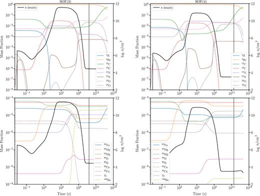
Mass fractions and neutron densities (n cm−3) of the hot SOFs of Cases 3 (left-hand panel) and 4 (right-hand panel), calculated at T = 123 MK and ρ ≈ 3 × 10⁴ g cm−3. The dashed vertical line is when the 16O/18O drops to its minimum value of ≈2, and the hot SOF abundances are taken at this point.
The four cases are listed in Table 2 and the abundances of the SOF and envelope for each case are listed in Table 3. The algorithm for the construction of each case is as follows:
(1) select the mass of the H-rich envelope of the He WD and homogenize the isotopic abundances over the mass of the He WD. The CO WD abundances are fixed for all initial models (Table 1).
The four cases. Abundances in the last two columns are initial amounts in the SOF and envelope, and are listed in Table 3.
| Case | H-envelope mass | SOF conditions | SOF abundances | Envelope abundances |
|---|---|---|---|---|
| 1 | 6.4 × 10⁻³ | Cold | SOF (1) | Envelope (1) |
| 2 | 1.0 × 10⁻² | Cold | SOF (2) | Envelope (2) |
| 3 | 6.4 × 10⁻³ | Hot | SOF (3) | Envelope (1) |
| 4 | 1.0 × 10⁻² | Hot | SOF (4) | Envelope (2) |
Isotopic mass fractions of the SOF and envelope regions for the initial post-merger models. The composition of the material dredged-up from the CO WD is the same for all SOFs and envelopes as in Table 1. SOF(1): cold, from He WD(1), SOF(2): hot, TSOF = 123 MK, from He WD(1), SOF(3): cold, from He WD(2), SOF(4): hot, TSOF = 123 MK. Envelope(1): from He WD(1) and Envelope(2): from He WD(2).
| Species | SOF(1) | SOF(2) | SOF(3) | SOF(4) | Envelope(1) | Envelope(2) |
|---|---|---|---|---|---|---|
| 1H | 3.7 × 10⁻³ | 7.1 × 10⁻³ | – | – | 6.6 × 10⁻³ | 1.3 × 10⁻² |
| 4He | 0.95 | 0.95 | 0.93 | 0.86 | 0.98 | 0.98 |
| 12C | 4.1 × 10⁻² | 4.1 × 10⁻² | 9.4 × 10⁻³ | 7.7 × 10⁻² | 7.8 × 10⁻³ | 7.8 × 10⁻³ |
| 13C | – | – | – | – | – | – |
| 14N | 9.3 × 10⁻⁴ | 9.2 × 10⁻⁴ | 1.6 × 10⁻³ | 1.7 × 10⁻² | 1.0 × 10⁻³ | 1.0 × 10⁻³ |
| 15N | – | 1.6 × 10⁻³ | 4.0 × 10⁻⁴ | 3.6 × 10⁻⁴ | – | – |
| 16O | 5.2 × 10⁻³ | 5.2 × 10⁻³ | 3.0 × 10⁻² | 2.0 × 10⁻² | 1.0 × 10⁻³ | 1.0 × 10⁻³ |
| 18O | – | – | 2.1 × 10⁻² | 1.6 × 10⁻² | – | – |
| Maximum neutron density (n cm−3) | – | – | 6.3 × 10¹¹ | 7.9 × 10¹⁰ | – | – |
(2) Mix the He and dredged-up CO WD abundances in proportions according to the description of the four zones in Section 2.1.
(3) Treatment of SOF: cold or hot? If cold, proceed to post-merger evolution (SOF(1) and SOF(2) in Table 3).
(4) If hot (Fig. 2), burn the SOF abundances at constant T, ρ conditions, until 16O/18O is of the order of 1–10 (SOF(3) and SOF(4) in Table 3).
(5) Use these SOF abundances in the initial model, with appropriate buffer and envelope abundances (Table 2) and begin post-merger evolution.
The four initial models are: Cases 1 and 2 which differ by the H-rich envelope mass of the He WD used to build them. Both of these are ‘cold SOF’ cases, i.e. the SOF is not burnt prior to the evolution. Cases 3 and 4 are ‘hot SOF’ cases. Case 3 is constructed with the abundance of Case 1 in the core, intershell, and envelope, but the SOF abundance from Case 1 is burnt until the 16O/18O drops to its lowest value . Case 4 is built in the same way as Case 3 but by using the initial abundances of Case 2.
2.3 Simulation algorithm
We used three codes for our work: nucleosynthesis codes from th e NuGrid family; the single zone frame (Herwig et al. 2008), and the multizone post-processing frame (Pignatari et al. 2016; Ritter et al. 2018), and the stellar evolution code mesa (version 6794) (Paxton et al. 2015).
For burning the SOF prior to constructing the initial model, we used the single-zone frame of NuGrid. Once the initial model was built, we used mesa to perform the stellar evolution calculations. The above initial profiles are relaxed onto a |$0.9\, \mathrm{M}_{\odot} \,$| pre-main-sequence model and then evolved until it passes through the region in the HR diagram where RCB stars are found: |$3000\, \mathrm{K}\le {T}_\mathrm{eff}\le 8000\, \mathrm{K}$| and |$3.5\le \mathrm{log}\, L/\mathrm{L}_{\odot}\le 4.0$| (Clayton 1996; Pandey et al. 2008) – this is the RCB phase of the model. We select the Blöcker’s mass-loss formula (Bloecker 1995) with η = 0.02 when the star reaches the RCB phase and Type I OPAL tables to calculate opacities. Energy generation is followed using an 18-isotope network that follows hydrogen- and helium-burning reactions.
The models were then post-processed using the multizone post-processing network frame of NuGrid. Each zone of a model computed at every time-step is processed with an adaptive nuclear network that uses over 1000 isotopes, taking also into account the diffusive mixing processes in the mesa model.
3 RESULTS
The evolutionary tracks are similar to those in fig. 5 ofPaper I. The RCB phase of our four post-merger models is between 6.7−9.2 × 10⁴yr, which is consistent with the expected lifetime of the order of 104–105 yr from observations.
3.1 Nucleosynthesis and mixing processes in the models
We examine the different phases of nuclear burning during the evolution of the models and how both burning and mixing simultaneously affect their surface abundances. In Paper I, the evolution of species from 1H to 22Ne were studied in detail. These species affected the 16O/18O and 12C/13C ratios and the abundance of 19F, as these formed the main focus of that work. The nature of the evolution of the above species is the same in the cases presented in this work as well (see Section 3.2.2, Paper I).
In this work, we examine the heavier species, such as the isotopes of Si, S, and Ca, using Case 1 to demonstrate their evolution (Fig. 3). There are two stages of nuclear burning: H-shell burning followed by He-shell burning. During the post-merger evolution of the models the maximum temperatures for H burning are between 40 and 50 MK and for He burning up to ∼250 MK. In Fig. 3, we show temporal snapshots of mass profiles of Case 1, with the diffusion coefficient of mixing (D) along with the convective region (the grey shaded portion), the neutron density (in n cm−3), and the isotopic abundance of 1H, 13C, 14N, 29Si, 30Si, and 32S. The temperature–density profiles of our models are similar to those of Paper I and the reader is referred to fig. 7 of Paper I for these.
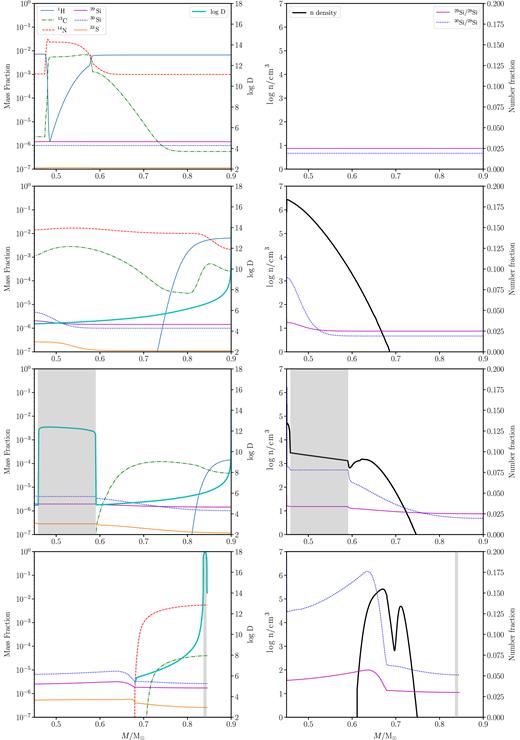
Snapshots of time for Case 1 from top to bottom: close to initial at t = 0.13 Myr, t = 0.32 Myr, t = 0.50 Myr, and at the termination of the evolution at t = 1.8 Myr. Left: mass fractions and diffusion coefficient (D) against mass coordinate. Right: neutron density (n cm−3) and number ratios of silicon isotopes against mass coordinate. Convection is shows as the grey shaded region. Since the mixing is restricted to the layers above the CO core, the mass range in this plot is restricted to |$0.45\text{-}0.90\, \mathrm{M}_{\odot} \,$|.
The region which participates in nuclear burning during the evolution of the post-merger model, i.e. the mass above the CO core, has |${\sim }98\text{-}99{{\ \rm per\ cent}}$| of He (not shown in the snapshots of Fig. 3), |$\lt\!\! 1.5{{\ \rm per\ cent}}$| of H, and |${\sim }0.3{{\ \rm per\ cent}}$| of metals. The first panel of Fig. 3 shows an early stage of post-merger evolution (t = 0.13 Myr). By 0.32 Myr, the second panel of Fig. 3, H has been completely burnt in the inner region of the star (|$0.45\lt M/\, \mathrm{M}_{\odot} \, \lt 0.7$|) and the H-shell moves toward the surface. The overall abundance of 14N has increased due to proton and neutron capture by 13C, and its simultaneous mixing upto the surface. This is also the period where the Ne–Na cycle is active and 23Na is created via 22Ne(p, γ)23Na (not shown in plot). 13C is also destroyed by He burning via 13C(α, n)16O, which gives rise to the formation of a neutron pocket (right-hand side of second panel). By 0.50 Myr, the third panel of Fig. 3, temperatures have become hot enough for He burning to become dominant and 13C is entirely destroyed in the interior of the star. At this time, the neutron pocket is diluted and spread over a mass of |$0.45\text{-}0.58\, \mathrm{M}_{\odot} \,$| by a convection zone which arises due to the triple-α reaction (right-hand side of third panel). 28Si undergoes neutron capture in this region to produce 29Si, while 30Si is produced more abundantly than 29Si, through the more efficient neutron-capture reaction of 33S(n, α)30Si. All these products from H and He burning, are gradually dredged up from the interior to the surface by the artificial mixing process we implement.
This diffusion coefficient is constructed such that it cuts off at the entropy barrier arising from the peak of nuclear energy in the star, which in our models is at approximately the location where 14N undergoes He capture to form 18O. Therefore as the model evolves, the 14N abundance profile burns and moves closer to the surface with the diffusion coefficient following simultaneously. By the time the star enters the RCB phase, mixing becomes restricted to the outer region of the model. By the end of the RCB phase, the fourth panel of Fig. 3, the post-merger star is 1.8 Myr for Case 1 and the 30Si/28Si in the surface is enhanced by twice its initial amount, while 29Si/28Si is not significantly enhanced compared to its initial value. About 0.05|$\, \mathrm{M}_{\odot}$| is lost from the surface due to winds. The duration of the RCB phase of this model is 9.2 × 10⁴ yr.
In Fig. 4, we use Ca isotopes to illustrate the evolution of neutron-capture species and simultaneously examine the differences between hot and cold SOF Cases, 1 and 3 respectively. Initially, Case 3 is more enriched in neutron-capture isotopes due to the contribution of the initially burnt SOF than Case 1 (Fig. 4, top panel). One of the first He-burning reactions to occur is 13C(α, n)16O, which gives rise to a neutron pocket (Fig. 4, second panel). In Case 1, the neutron pocket reaches a maximum density of ≈2.5 × 10⁶ n cm−3 and spans a broader mass zone than Case 3 whose maximum neutron density is ≈6.3 × 10⁴ n cm−3. The weaker neutron pocket of Case 3 produces a lower enhancement in the 43Ca/40Ca ratio than Case 1 (Fig. 4, third panel); thus in Case 3, the change in the surface value of this ratio is primarily due to the artificial mixing which dredges up the hot SOF abundances (Fig. 4, bottom panel). On the other hand in Case 1, the 43Ca/40Ca ratio is affected by neutron capture occurring during the post-merger evolution. The isotopes of Ti evolve in a similar way as Ca isotopes. Neutron-capture reactions also produce Ni and Zn in our models.
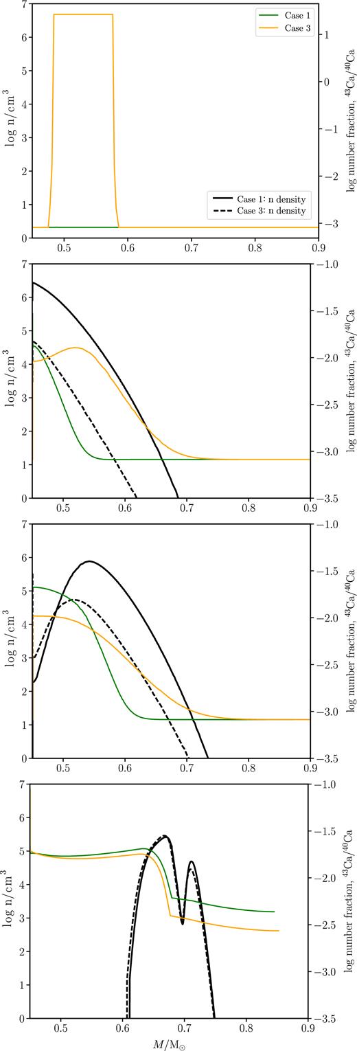
Snapshots of time for Cases 1 and 3, showing the evolution of the number fraction of Ca isotopes and neutron density (n cm−3). From top to bottom, Case 1 (Case 3): t = 0.13 (0.11) Myr, t = 0.32 (0.28) Myr, t = 0.34(0.31) Myr, and t = 1.8(1.7) Myr.
Prior to examining the evolution of individual elements that have been observed in RCB stars, we discuss the structural differences between the four cases during their evolution. The main difference between Cases 1 and 2 initially is their H abundance, with Case 2 having a higher H abundance than Case 1. During their evolution, the wide convection zone between |$0.45\text{ and }0.58\, \mathrm{M}_{\odot} \,$| which arises in Case 1 (third panel, Fig. 3), does not appear during the evolution of Case 2. Both these cases attain nearly the same maximum neutron densities during their evolution, but as the wide convection zone in Case 1 causes the neutron pocket to be spread out, it produces a larger abundance of neutron-capture isotopes in Case 1 than Case 2.
The main difference between the cold (Cases 1 and 2) and their corresponding hot SOF cases (Cases 3 and 4) is that in the cold SOF cases, all the nuclear-burning processes occur during the post-merger evolution of the star. In the hot SOF models, the abundances of the SOF zone of the initial profile were burnt prior to the beginning of the evolution and hence these SOFs (Fig. 2) are enriched in products of He burning and neutron capture.
3.2 Elemental abundances and comparison with RCB stars
The products of H burning during the evolution of the post-merger model are: 13C, 14N, and 23Na and in the setup of the hot SOF is 25Mg (Fig. 2). The products of He burning are: 16O, 18O, 15N, 19F, 22Ne, and neutrons. Depending on the neutron density during the post-merger evolution the isotopes of Si, Ti, Ca, Ni, Zn, and the elements of the first s-process peak Y and Zr are affected. The prior burning of the hot SOFs also affects the abundance of these isotopes and depending on the neutron density during their burning, can also significantly enhance the abundance of the second s-process peak elements Ba and La.
We next discuss the evolution of those elements in our models that have been observed in RCB stars.
Carbon is predominantly in the form of 12C in our models, which is already larger than 13C in the initial composition (12C/13C = 325 initially), and is then increased further due to the triple-alpha reaction. 13C is first consumed by proton capture to make 14N and then entirely destroyed due to alpha capture through 13C(α, n)16O. The net effect of these processes is that the 12C/13C ratio at the surface is increased significantly. Since the SOFs of the hot SOF models are entirely depleted in 13C (Table 3), the final 12C/13C ratio at the surface of the hot SOF cases is higher than their corresponding cold SOF cases.
Nitrogen is constituted of 14N and 15N in our models. Aside from the contribution of the He WD (Table 1), 14N is also created in the star from 13C(p, γ)14N and then destroyed by He burning through 14N(α, γ)18F(+β, γ)18O. 14N is a neutron poison and creates protons through 14N(n, p)14C, which allows for the production of 15N through He burning, via 18O(p, α)15N. 15N is destroyed by further He burning through 15N(α, γ)19F. The SOFs of the hot SOF cases produce some 15N (Table 3) and hence these cases are initially more enhanced in 14N/15N than the corresponding cold SOF cases.
Oxygen in our models is predominantly 16O followed by 18O and 17O. The 16O/18O number ratio from the initial composition is 1417 and that of 16O/17O is 6800. Proton capture by 16O produces 17O via 16O(p, γ)17F(+β, γ)17O. 16O is initially enhanced in all cases due to alpha enhancement of the initial composition, and is then further produced by 12C(α, γ)16O and 13C(α, n)16O in the star. He burning of 14N produces 18O in the star and also in the SOFs of the hot SOF cases (Table 3) leading to an overall initial enhancement of this ratio in Cases 3 and 4.
Fluorine is created in the star by the destruction of 15N via 15N(α, γ)19F.
Sodium is enhanced from its initial amount due to the reaction 22Ne(p, γ)23Na from the Ne–Na cycle, during the evolution of the post-merger model. Only one of the stable isotopes of Magnesium, 25Mg, is produced in nominal amounts during the post-merger evolution at the maximum temperatures of H burning at 40–50 MK, via 24Mg(p, γ)25Al(+β, γ)25Mg. It is also enhanced in the hot SOFs.
Aluminium is negligibly affected during the post-merger evolution or in the hot SOFs since the temperatures of 40–50 MK are not sufficient for hot H burning via the Mg–Al chain. 25Mg(p, γ)26Al weakly creates some 26Al. Temperatures of >50 MK are required to activate the Mg–Al chain for producing significant amounts of Al (Arnould, Goriely & Jorissen 1999; Iliadis 2007).
We now come to elements whose isotopes are affected only by neutron capture.
The maximum values for the neutron densities are in the range of 105–107 n cm−3 during the evolution of the four post-merger cases. On the other hand, the SOFs when burnt prior to the evolution of Cases 3 and 4 produce higher maximum neutron densities of 6.3 × 10¹¹ n cm−3 in the SOF of Case 3 and 7.9 × 10¹⁰ n cm−3 in the SOF of Case 4 (Fig. 2), upto a period of 107 s. Since for the initial setup of Cases 3 and 4, we take the SOF abundances at a much later time (≈1010 s) when the 16O/18O ratio drops to its lowest value, their SOFs are enriched in isotopes of neutron capture and He burning (Fig. 2 and Table 3), thus contributing to the overall enrichment of these species at the surface of the RCB models from Cases 3 and 4.
Silicon and sulphur are not produced in our models since temperatures required for their creation are of the order of 1 GK. Their isotopic ratios are however, affected by neutron captures as was shown in Fig. 3. Calcium and titanium are unchanged from their initial amounts except in Case 3 in which Ti is produced.
As the SOF of Case 3 has a lower initial H abundance than Case 4, only a smaller fraction of 13C is destroyed to 14N, making more 13C available for neutron production in the SOF of Case 3 compared to that of Case 4 (Table 3). Thus, the SOF of Case 3 has a larger maximum density of neutrons (6.3 × 10¹¹ n cm−3) than Case 4 (7.9 × 10¹⁰ n cm−3). The larger neutron density of Case 3 causes elements prior to the first s-process peak such as Ni and Zn, to undergo neutron capture and give rise to large enhancements in elements belonging to the s-process peak elements such as Y, Zr, Ba, and La. On the other hand, the neutron density in the SOF of Case 4 is high enough only to produce isotopes of Ni and Zn, and to a smaller extent in the s-process elements belonging to the first s-process peak, Y and Zr. Thus the net surface abundances of Ni and Zn are higher in Case 4, while those of the s-process elements are higher in Case 3. Ba and La which are second peak s-process elements, are not produced in the SOF of Case 4.
To summarize, Cases 1 and 3 have a lower initial abundance of hydrogen than Cases 2 and 4 respectively and hence have more 13C, higher neutron densities and less 14N. Consequently, Cases 1 and 3 produce higher amounts of neutron-capture isotopes than Cases 2 and 4. On the other hand, the abundance of proton-capture isotopes such as 14N, 15N, 17O, and 25Mg are higher in Cases 2 and 4 owing to their larger H abundance than Cases 1 and 3, respectively.
We next compare individual elemental abundances between our models and those of RCB stars, taken from the database compiled by Jeffery et al. (2011), (which is itself based on the data of Asplund et al. 2000 and Pandey et al. 2008) and which was also used in Paper I. RCB stars were classified as minority and majority stars by Lambert & Rao (1994) based on their abundances – the RCB minority stars (black squares in Fig. 5) have a lower [Fe] abundance and higher Si/Fe and S/Fe values than the RCB majority stars (black stars in Fig. 5). We use the same notation as Jeffery et al. (2011) to represent the elemental abundances; the abundance [X] is calculated as [X] = εi,⋆ − ε⊙,i, where |$\epsilon _\mathrm{i} \equiv \mathrm{log}\, n_\mathrm{i}+C$|, C being a constant and ni the number density of species i. The individual errors are not marked in Fig. 5, but there is a general uncertainty of ±0.2–0.3 dex in the measured abundances.
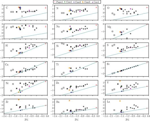
Comparison of the surface abundance of the four cases in this work, with observed abundances of RCB stars. We use the same symbols as in fig. 12 of Paper I. Black square symbols are RCB minority stars and black star symbols are RCB majority stars; the two filled square symbols have 16O/18O measured from García-Hernández et al. (2010). As a reference we also plot the abundances of Case 1 of Paper I as the + symbol. The prototype, RCrB is the pink ⋆. Cases 1 and 3 are plotted as filled green and orange ○ symbols respectively, and Cases 2 and 4 as filled blue and purple △ symbols, respectively. The grey ⊕ symbol is the abundance from the initial Z = 0.0028 alpha-enhanced composition. The teal-dashed line shows the scaled-solar composition.
For the purpose of our analysis, we divide the elements as those that are primarily affected by neutron capture and those that are not. We begin with the ones whose isotopes are not affected by neutron-capture reactions: C, N, O, F, Na, and Mg. Their abundances are determined mainly by H- and He-burning reactions within the star. In the observations of RCB stars, the [X] values of these elements seem to not have a distinct correlation with metallicity, until [Fe] < −1.5 dex, and then decrease as [Fe] decreases. Both our new metal-poor models and the solar-metallicity model of Paper I, obtain elemental abundances of these elements close to the upper limits of the values observed in RCB stars.
In our models, the abundance of C is enhanced up to 2 dex, N up to 1 dex, and O up to 1.2 dex, all compared to solar. Carbon is overproduced in our models because of two reasons- the initial enhancement [C/Fe] = 0.55 dex and its production in the star due to the triple-alpha reaction. This 12C is burnt to 16O through alpha capture, and hence the [O] values are also in the upper limit of the observed range. Nitrogen is enhanced due to the contribution of 14N in the initial setup from the He WD and the hot SOFs (Tables 1 and 3) and the production of 14N and 15N during the evolution of the star and from the hot SOFs as well.
Fluorine has only one stable isotope, 19F which is predominantly produced by the He burning of 15N in the star. Fluorine values are enhanced to 1–2.3 dex and reasonably span the entire observed range as did the solar-metallicity models of Paper I.
Sodium is enhanced in our models due to H burning in the Ne–Na cycle in the early stages of the evolution and its abundance matches the abundances measured in RCB stars. Case 4 makes the highest amount of Na because of the contribution of 22Ne seed nuclei from its hot SOF which then undergo proton capture during the post-merger evolution. The abundances of Mg and Al are unchanged from their initial alpha-enhanced values in our models because temperatures are not hot enough for the Mg–Al chain to operate. The observed abundances of Na, Mg, and Al in RCB stars scale down with [Fe] more or less the same way as the solar-scaled composition (the dashed teal line in Fig. 5) down to [Fe] = −1.5 dex. Lower than [Fe] = −1.5 dex, the elemental abundances of the three RCB stars appear more enhanced in [X/Fe] than their more metal-rich counterparts. For [X/Fe], we compare the offset of [X] against the dashed teal line. Thus, C, N, O, F, and Na are substantially produced in our models, while Mg and Al reflect only their initial values. Despite not being produced in our models, the initial abundance of Mg is sufficient to match the observational data.
The abundances of Si, S, and Ca are unchanged from their initial values since temperatures high enough for O burning are required to produce them. Calcium is in fact, very close to the solar-scaled value for most of the RCB stars, except two stars that have a lower metallicity than our models and show enhancements of [Ca/Fe] ≈ 0.8 dex. Titanium is significantly enhanced to match the observed values only in Case 3 due to the contribution of its hot SOF.
Nickel isotopes are produced by neutron capture in our models, causing an enhancement of ∼0.4 dex in Case 4 (through its hot SOF) and ∼0.3 dex in Case 1, compared to the initial amount. These values are not sufficiently high to match the abundances of Ni in RCB stars. The production of large amounts of Ni, like Si and S requires temperatures of at least |${\sim }1\,$|GK. Zinc is sufficiently produced to match the observed abundances, again from the SOF of Case 4.
S-process elements Y, Zr, Ba, and La are greatly enhanced by up to 2–2.5 dex compared to solar in Case 3. These values however, are much higher than observations. Cases 1 and 4 produce the required abundances of these elements that match the observations.
Our best RCB model whose surface abundances are within range of most species observed in RCB stars, is from Case 4.
3.3 Comparison with pre-solar graphite grains
In Figs 6–8, we compare the number ratios of isotopes from our models with the observed LD graphite grain data, taken from the pre-solar grain database of Hynes & Gyngard (2009). In Figs 7 and 8, we use the δ notation to represent the isotopic ratios. It is calculated as follows: δ(iX/jX) = ((iX/jX)⋆/(iX/jX)⊙) − 1) × 1000.
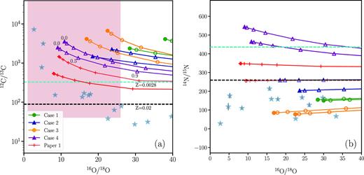
Number ratios of (a) 12C/13C and (b) 14N/15N against 16O/18O. The grain data are the grey stars along with error bars. Error bars for 16O/18O are within the symbol. Dilution lines connect points that represent different fractions of dilution with solar material; filled symbols are directly taken from the surface of the models (without any dilution); and empty symbols represent dilution with 0.1, 0.3, 0.5, 0.7, 0.9, and 1.0 fraction of solar composition. The dashed cyan line is the value for the alpha-enhanced composition at Z = 0.0028 and dashed black line is the solar composition. The shaded region in (a) represents the observed limits for RCB stars; the lower bound for 12C/13C is set to 40 (Hema et al. 2012) and 16O/18O is set to 1–25 (Clayton et al. 2007; García-Hernández et al. 2010). Note: the measurements for these two ratios were obtained independently and do not belong to the same stars. Symbols and lines of this figure are used in the following figures Figs 7 and 8. Error bars for 16O/18O are so small that they are within the symbol. Note also that not all data points have error bars.
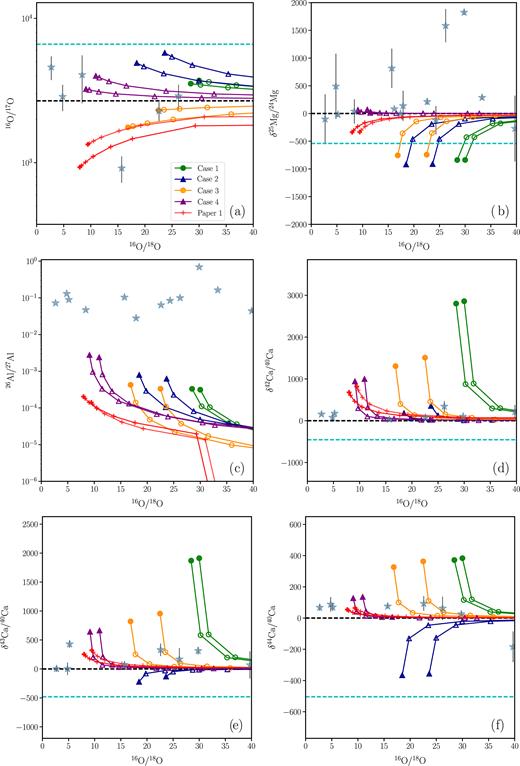
Number ratios of (a) 16O/17O and (c) 26Al/27Al, and δ-values of (b) 25Mg/24Mg number ratio, and (d)–(f) of Ca isotopes versus 16O/18O for our models and the grains.
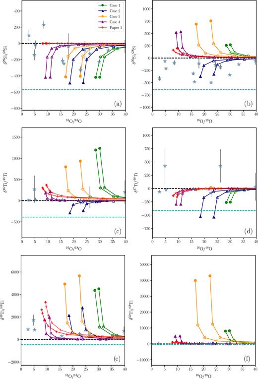
δ-values of (a) and (b) Si isotopes, (c)–(f) Ti isotopes versus 16O/18O for our models and the grains.
Although the 16O/18O ratio measured in RCB stars is less than 25, we expand the range of grain data to include those with 16O/18O < 40, since Case 1 has 16O/18O = 29–33. Due to the uncertainty in the physics of grain condensation, we assume that the gas ejected by an RCB star can be mixed with different proportions of interstellar material of solar composition before condensing into carbon dust. We hence also investigate the effect of dilution with solar material on the surface isotopic ratios of our four RCB models and how they compare with the grain composition. Each of our cases has two points, one representing the value at the start of the RCB phase and one when it leaves the RCB phase on the HR diagram. We also plot dilution lines which represent the isotopic number ratio on diluting the values from the surface of the models with different fractions of the solar value. Diluted ratios are calculated for fractions of 0.0 (direct surface value of the ratio from the model), 0.1, 0.3, 0.5, 0.7, 0.9, and 1 (solar value, not visible since the x-axis range is restricted to 16O/18O ≤ 40). As the ratios become increasingly diluted with solar mass fractions, the dilution lines move toward the right of the figures and asymptotically approach the solar composition (horizontal dashed black line).
There are only two common isotopic ratios that have been measured between RCB stars and LD graphite grains: 12C/13C and 16O/18O (Fig. 6a). Cases 2 and 4 which are constructed with the higher initial H-abundance, make more 14N through 13C(p, γ)14N and thus make more 18O than Cases 1 and 3, respectively. Hence, Case 2 has 16O/18O in the range of 19–23, while Case 1 has a larger range of 29–33 at the surface. Introducing a burnt SOF in the initial setup, decreases this ratio in the hot SOF cases to 9.5–10.2 in Case 4 and 17–23 in Case 3.
The models have much higher values of 12C/13C than the grains, between 1500 and 7000 as against the grain values which are in the range of 30–200. This is because of the high initial 12C/13C ratio of 325, the production of 12C and destruction of 13C due to He burning. Changing the H-envelope mass does not affect the 12C/13C ratio significantly. The hot SOF cases however are initially enhanced in 12C and depleted in 13C in the SOF region, and thus their final C-isotopic ratios at the surface are also higher than their corresponding cold SOF cases.
Ten grains in Fig. 6(a) which have 16O/18O<25 and 12C/13C>100, fall within the observational range of RCB stars. None of our models, however, can simultaneously produce the grain values in this region of 16O/18O and 12C/13C. Only three grains have 12C/13C ratios of 700–7400 which are comparable to the estimates from our models, but these grains also have very low 16O/18O ratios of 3–4. Our models however, only go down to 9.5 in 16O/18O.
One of the major successes of our models is in obtaining the sub-solar 14N/15N values measured in these graphite grains (Fig. 6b); our models have a range of 14N/15N = 70–540, three of which are below the initial amount of 14N/15N = 470. The 14N/15N ratio of Case 4 exceeds the initial value of 470, because of the production of 14N in the star and also from its initial hot SOF contribution.
The isotopes 17O, 25Mg, and 26Al are affected by proton capture reactions in our models. The 16O/17O ratio (Fig. 7a) is measured only for six grains in this set, and our models show a reasonable spread that matches the range in the grains.
Case 4 produces the highest amount of 25Mg compared to the other cases (Fig. 7b) and δ25Mg/24Mg is enhanced above the initial value of −590 due to its hot SOF (Fig. 2). Within the error bars of the data, Case 4 matches the measured values of δ25Mg/24Mg. Although 25Mg is produced in Cases 1–3, it is not enhanced above 24Mg. Diluting with 30 per cent of solar mass fractions can also make Cases 2 and 3 to match the data.
26Al is not produced sufficiently in our models to match the grain data, while 27Al remains at the initial amount in the models (Fig. 7c). The ratio of 26Al/27Al is 0.0003–0.003 in our models, while the grains have ratios of 0.03–0.7. Along with the C abundance, Al is also one of the key places where our models need to be improved.
Beginning with Si in Figs 8(a) and (b), we direct our attention to the neutron-capture isotopes in our models. The evolution of 29Si/28Si and 30Si/28Si have been illustrated in Fig. 3. Due to the higher initial hydrogen abundance and a wider convection zone that arises due to the energy released by the triple-α reaction during the evolution, the abundances of all neutron-capture isotopes are higher in Case 1 than Case 2. Hence, the abundances of 29Si and 30Si compared to 28Si are higher in Case 1 than Case 2. Owing to higher neutron densities in the SOF, the hot SOF Case 3 has higher abundances of neutron-capture isotopes than Case 4. All four of our models match the δ(29Si/28Si) ratio but have much higher values than the δ(30Si/28Si) measured in the grains, except for Case 2.
For the Ca isotopes (Figs 7d–f), diluting the abundances of Cases 1, 3, and 4 with 10–30 per cent solar material produces a reasonable match with the measured grain data. Case 2 is the least enhanced in neutron-capture isotopes, and matches the grain data without much dilution. The same trends are also observed in the Ti isotopes (Figs 8c–f). With a dilution of 10–30 per cent, Cases 2 and 4 can reproduce the observed δ values of all four Ti isotopes. Cases 1 and 3 are more enhanced in the Ti isotopic ratios and hence require higher dilution fractions of ≥30 per cent to match the grain data.
Except for the high values of 14N/15N, the case that reasonably matches the other measured isotopic ratios of our sample of graphite grains is Case 4.
4 DISCUSSIONS AND CONCLUSIONS
We have presented 1D stellar evolution models of RCB stars with an alpha-enhanced initial composition of Z = 0.0028, initiated from hybrid post-merger structures of CO + He WD mergers, by using the methodology of Menon et al. (2013, Paper I). Four cases were studied in the current work, which primarily differed by their initial hydrogen mass in the envelope and their SOF abundances. We followed the evolution of the post-merger models until they passed through the RCB phase in the HR diagram and compared their isotopic abundances from their surface with those observed in RCB stars.
Our post-merger models spent 6.7–9.2 × 10⁴ yr in the RCB phase, which is in line with the observational estimate of ≈104–105 yr (Clayton et al. 2011; Clayton 2012). Similar to the solar-metallicity RCB models of Paper I, the models in this work also have low 16O/18O ratios of 9.5 − 33, high 12C/13C ratios of >100, enhancements in F and s-process elements compared to solar, all of which are characteristic signatures of RCB stars. A key reason for the success of our models is the implementation of the artificial mixing routine, whose prescription and parametric values were adapted from Paper I.
Elements such as C, N, O, Mg, Al, Si, S, and Ca are not affected significantly by the choice of the H mass fraction or the SOF abundances. Fluorine, Na, Ti, Ni, and Zn show a more noticeable spread in abundance (≈0.8 dex) between the models. The s-process elements, Y, Zr, Ba, and La, show the largest variation in abundances between the models, particularly in Case 3 due to its lower initial H-abundance and its hot SOF. The presence of the hot SOF increases the abundance of s-process elements compared to the cold SOF cases, and also the n-capture isotopic ratios.
Carbon is overproduced in all our models and they only match the observed upper limits of N, O, and Na. The abundances of Al, Si, and S, are observed to be enhanced in RCB stars but remain unchanged in our models. Similarly, Mg and Ti (except Case 3) are unchanged in our models but they are within the limits of the observed range in RCB stars. The models also do not produce sufficiently high abundances of Ni or the observed spread in Ca abundances. Lithium which has been observed to be enhanced in a few RCB stars (Asplund et al. 2000), is not produced in our models.
We compare the isotopic composition of those LD graphite grains which have 16O/18O<25 and 12C/13C>100 which are similar to the range observed in RCBs. We explore the effect of dilution with solar material on the surface composition of our RCB models, under the hypothesis that the gas ejected by RCBs could mix with interstellar solar material before condensing as grains.
Three of our models can reproduce the sub-solar values of 14N/15N = 70–240 and match the grain values. They can also reproduce the low δ29Si/28Si ratios, which were attributed to the production of 28Si from massive stars and ejected in supernova explosions in earlier studies. In our low-metallicity models, 28Si is alpha enhanced in the initial composition and 29Si is weakly produced by neutron capture. The δ30Si/28Si ratios in our models are enhanced by neutron capture above the solar value, except for Case 2 which has a weak neutron pocket. The isotopic ratios of Ca and Ti isotopes are also enhanced above solar due to neutron capture, but these can be reduced to match with the grain data by diluting their abundances with at least 10 per cent of the solar mass fraction.
Our best model that reproduces most of the isotopic ratios and elemental abundances of RCB stars and some of the grain signatures, is Case 4. We rule out Case 3 due to the excessive amounts of s-process elements it produces compared to what is observed in RCB stars.
Carbon in our models is higher by nearly 1 dex compared to the observed value in RCB stars and the 12C/13C ratios in our models is between 1500 and 7000 while most of the grains have 12C/13C less than 100. Thus carbon is excessively produced in our models in comparison with both, RCB stars and the graphite grains. The abundance of carbon depends greatly on its enhancement in the initial composition. In our work, initial values of [C/Fe] = 0.55 dex and 12C/13C = 325 were chosen which are higher than the predictions from galactic chemical evolution models such as those of Kobayashi et al. (2011), and observations of stars in the solar neighbourhood. The latter show an uncertainty in the abundance prediction of carbon and can vary between [C/Fe] = −0.4 and 0.2 dex for the metallicity of Z = 0.0028 which we used for our models.
We do not produce the excess in δ25Mg/24Mg observed in the grains except for Case 4. We also do not produce sufficiently high amounts of 26Al that can match the 26Al/27Al ratios of 0.03–0.7 observed in the grains nor the enhancement of [Al] in RCB stars, of up to ≈0.5 dex compared to its initial value.
For our models to completely match all the elemental abundances of RCB stars and the isotopic ratios measured in the grains, we need to boost the production of 13C, 25Mg, and 26Al. One underlying mechanism can solve this problem – a layer of partial H burning close to the surface that does not mix with the He-burning layer below it. We did a rough test calculation for estimating whether this solution will work for 26Al in Case 2. The H-burning shell of ≈0.1 |$\, \mathrm{M}_{\odot}$| must sit on top of the SOF which has temperatures conducive for hot H burning i.e. of 60–100 MK, and densities of 1.6–2.5 × 10³g cm−3. On burning the envelope composition of Case 2 at T = 100 MK and ρ = 2 × 10³ g cm−3 for 106–1010 s, the mass fraction of 26Al increases to 3 × 10⁻⁶ and hence the mass of 26Al produced in the H-burning shell of 0.1 |$\, \mathrm{M}_{\odot}$| is 3 × 10⁻⁷. If all this 26Al is uniformly mixed in the entire envelope which has a mass of 0.32 |$\, \mathrm{M}_{\odot}$| , the mass fraction of 26Al in the envelope is 3 × 10⁻⁷/0.32 = 9.4 × 10⁻⁷. The abundance of 27Al is unchanged at these T, ρ conditions and hence its envelope abundance is the same as the initial value of 4 × 10⁻⁶. Thus, the number ratio of 26Al/27Al in the envelope is (9.4 × 10⁻⁷/4 × 10−6) * (27/26) = 0.244. Our target for this ratio according to the grain data is of the order of 0.1, which we achieve by this calculation. The same calculation for 25Mg can also produce high values of δ25Mg/24Mg that will match the grain data.
This calculation however does not produce sufficient amounts of 13C that can reduce the 12C/13C number ratios in our models. This once again indicates that the initial carbon value and the 12C/13C ratio used in our calculations were quite high. In a test calculation we did for Case 1, in which the initial 12C and 16O were reduced by an order of magnitude, thus reducing the initial 12C/13C and 16O/18O ratios, but keeping the same initial ratio of carbon to oxygen, the final surface ratio of 12C/13C was ≈ 95 compared to 2000 but 16O/18O increased to 47 compared to 29–33. Thus, the final surface ratios of 12C/13C and 16O/18O are highly sensitive to their initial quantities.
In conclusion, our new low-metallicity stellar evolution models for post CO + He WD merger structures, match most of the chemical signatures of RCB stars quite well, particularly the low 16O/18O ratios. The models are sensitive to the initial setup – the final surface abundances depend on the initial H-mass present in the star and the treatment of the SOF. The model predictions are in partial agreement with some of the LD graphite grain data, and show promise in being sources of LD graphite grains with low 16O/18O ratios.
ACKNOWLEDGEMENTS
The authors thank the referee for comments that helped improve the clarity of the paper. ML and CLD are supported by the Momentum ‘Lendület-2014’ Programme of the Hungarian Academy of Sciences.
