


ABSTRACT
We present a detailed X-ray timing analysis of the highly variable narrow-line Seyfert 1 (NLS1) galaxy IRAS 13224–3809. The source was recently monitored for 1.5 Ms with XMM–Newton, which, combined with 500 ks archival data, makes this the best-studied NLS1 galaxy in X-rays to date. We apply standard time- and Fourier-domain techniques in order to understand the underlying variability process. The source flux is not distributed lognormally, as expected for all types of accreting sources. The first non-linear rms–flux relation for any accreting source in any waveband is found, with rms ∝ flux2/3. The light curves exhibit significant strong non-stationarity, in addition to that caused by the rms–flux relation, and are fractionally more variable at lower source flux. The power spectrum is estimated down to ∼10−7 Hz and consists of multiple peaked components: a low-frequency break at ∼10−5 Hz, with slope α < 1 down to low frequencies, and an additional component breaking at ∼10−3 Hz. Using the high-frequency break, we estimate the black hole mass |${M_{\rm {BH}}}= [0.5{--}2] \times 10^{6} {\, \mathrm{M}_{\odot }}$| and mass accretion rate in Eddington units, |${\dot{m}_{\rm Edd}}\gtrsim 1$|. The broad-band power spectral density (PSD) and accretion rate make IRAS 13224–3809 a likely analogue of very high/intermediate-state black hole X-ray binaries. The non-stationarity is manifest in the PSD with the normalization of the peaked components increasing with decreasing source flux, as well as the low-frequency peak moving to higher frequencies. We also detect a narrow coherent feature in the soft-band PSD at 7 × 10⁻⁴ Hz; modelled with a Lorentzian the feature has Q ∼ 8 and an rms ∼3 per cent. We discuss the implication of these results for accretion of matter on to black holes.
1 INTRODUCTION
Accretion of matter on to supermassive black holes (SMBHs), with mass |${M_{\rm {BH}}}\sim 10^{5-9} {\, \mathrm{M}_{\odot }}$|, powers active galactic nuclei (AGNs) via the conversion of gravitational energy into radiation. (Lynden-Bell 1969; Malkan & Sargent 1982). The accretion process should be entirely described by the black hole (BH) mass and spin (Shakura & Sunyaev 1973), but their observational appearance will also be determined by the mass accretion rate, geometry, and other system parameters. The underlying emission mechanisms are believed to be relatively well understood; however, details about the geometry and location of the emission components are still unclear.
AGNs vary at all wavelengths and on all time-scales observed so far, with the largest and most rapid variations observed in the X-ray band (see e.g. Padovani et al. 2017 for a review). Variations in X-ray amplitude are observed on time-scales as short as ∼100 s (e.g. Vaughan et al. 2011), implying a small X-ray emission region (e.g. Mushotzky, Done & Pounds 1993). Understanding the variability process is crucial both to understanding the accretion process and to determining the fundamental properties of the central BH. The variability provides an orthogonal and complementary dimension to time-averaged spectral studies for understanding the source properties (see e.g. McHardy 2010; Uttley et al. 2014).
X-ray light curves in AGNs display a linear relationship between the rms amplitude of short-term variability and flux variations on longer time-scales (e.g. Gaskell 2004; Uttley, McHardy & Vaughan 2005; Vaughan et al. 2011), known as the ‘rms–flux relation’ (Uttley & McHardy 2001; Uttley, McHardy & Vaughan 2017). This appears to be a universal feature of the aperiodic variability of accreting compact objects. It is seen in neutron star and BH X-ray binaries (XRBs; e.g. Gleissner et al. 2004; Heil, Vaughan & Uttley 2012) and ultraluminous X-ray sources (ULXs; Heil & Vaughan 2010; Hernández-García et al. 2015). Linear rms–flux relations are also seen in the fast optical variability from XRBs (Gandhi 2009) and blazars (Edelson et al. 2013), as well as accreting white dwarfs (Scaringi et al. 2012) and young stellar objects (Scaringi et al. 2015).
The leading model to explain this variability property is based on the inward propagation of random accretion rate fluctuations in the accretion flow (e.g. Lyubarskii 1997; Kotov, Churazov & Gilfanov 2001; King et al. 2004; Zdziarski 2005; Arévalo & Uttley 2006; Ingram & Done 2010; Kelly, Sobolewska & Siemiginowska 2011, Ingram & van der Klis 2013; Cowperthwaite & Reynolds 2014; Scaringi 2014; Hogg & Reynolds 2016). Turbulent fluctuations in the local mass accretion rate at different radii propagate through the flow, with variability coupled together over a broad range in time-scales.
The long-time-scale X-ray variability of accreting BHs displays delays in the variations of harder energy bands with respect to softer energy bands (Miyamoto & Kitamoto 1989; Nowak et al. 1999a,b; Vaughan et al. 2003b; McHardy et al. 2004; Arévalo, McHardy & Summons 2008; Alston, Done & Vaughan 2014a; Lobban, Alston & Vaughan 2014). These hard-band lags can also be explained by the model of inward propagation of mass accretion rate fluctuations (Arévalo & Uttley 2006). On faster time-scales, AGNs show soft-band time lags with respect to continuum-dominated bands (e.g. Fabian et al. 2009; Emmanoulopoulos, McHardy & Papadakis 2011; Alston, Vaughan & Uttley 2013; De Marco et al. 2013; see Uttley et al. 2014 for a review). This reverberation signal has been interpreted as reprocessing of the intrinsic coronal X-ray emission (e.g. Uttley et al. 2014).
The focus of this paper is the narrow-line Seyfert 1 (NLS1) galaxy IRAS 13224-3809, a nearby (z = 0.066) X-ray-bright (4 × 10⁻¹² erg s−1 cm−2 in the 0.3–10.0 keV band; Pinto et al. 2018), radio-quiet NLS1 galaxy (1.4 GHz flux of 5.4 mJy; Feain et al. 2009). It is one of the most X-ray-variable NLS1 galaxies known, showing large amplitude variability in all previously targeted observations: ROSAT (Boller et al. 1997); ASCA (Dewangan et al. 2002). IRAS 13224–3809 was first observed with XMM–Newton in 2002 for 64 ks (Boller et al. 2003; Gallo et al. 2004; Ponti et al. 2010). A 500 ks observation in 2011 (Fabian et al. 2013) revealed a flux dependence to the X-ray time lags, with the reverberation signal observed at lower fluxes only (Kara et al. 2013).
IRAS 13224–3809 was recently the target of a very deep observing campaign with XMM–Newton, with observations totalling 1.5 Ms, as well as 500 ks simultaneously with NuSTAR . Results from this campaign so far include the discovery of flux-dependent ultrafast outflow (UFO; Parker et al. 2017b). The UFO varies in response to the source continuum brightness (Pinto et al. 2018). This variable outflow has also been revealed through variable emission-line components seen with principal component analysis (PCA; Parker et al. 2017a). Its X-ray spectrum shows a soft continuum with strong relativistic reflection and soft excess (Ponti et al. 2010; Fabian et al. 2013; Chiang et al. 2015; Jiang et al. 2018). The relationship between the variable X-ray and ultraviolet (UV) emission was explored in Buisson et al. (2018). The UV was found to have a low fractional variability amplitude (∼2 per cent on time-scales ≲ 10−5 Hz) and no significant correlation was found between the X-ray and UV emission, which is typical of high-accretion-rate Seyferts (e.g. Uttley 2006; Buisson et al. 2017).
This paper is the first in a series on the X-ray variability properties of IRAS 13224–3809. We explore the underlying variability processes occurring across a broad time-scale. In Section 2 we describe the observations and data reduction. In Section 3 we explore the flux distribution and stationarity of the light curves and present the rms–flux relation. In Section 4 we present the power spectral density and its energy dependence. In Section 5 we discuss the results in terms of the variability processes dominating the inner accretion flow.
2 OBSERVATIONS AND DATA REDUCTION
IRAS 13224–3809 was the subject of an intense XMM–Newton VLP proposal (PI: Fabian) observed 12 times over 30 d during 2016 May–June, with a total exposure ∼1.5 Ms. We also use four earlier observations taken in 2011, totalling ∼500 ks (see Fabian et al. 2013), and a 64 ks observation from 2002 (see e.g. Gallo et al. 2004). This paper uses data from the EPIC-pn camera (Strüder et al. 2001) only, due to its higher throughput and time resolution. The raw data were processed from Observation Data Files (ODFs) following standard procedures using the XMM–Newton Science Analysis System (sas; v15.0.0), using the conditions PATTERN 0–4 and FLAG = 0. The 2016 and 2011 EPIC observations were made using large-window mode. The source counts were extracted from a circular region with radius 20 arcsec. The background is extracted from a large rectangular region on the same chip, placed away from the source. For observations taken in large-window mode we avoid the Cu ring on the outer parts of the pn chip.
We assessed the potential impact of pile-up using the sas task EPATPLOT (Ballet 1999; Davis 2001). A small amount of pile-up is found during the highest flux periods (see also Pinto et al. 2018; Jiang et al. 2018), which we find has no effect on the timing analysis throughout. Strong background flares can affect timing results, particularly at high energies, so particular care has been taken to remove the influence of flaring and background variations (which are typically worse at the beginning and end of XMM–Newton observations). Following Alston et al. (2013, 2014b), for flares of duration ≤200 s the source light curve was cut out and interpolated between the flare gap by adding Poisson noise using the mean of neighbouring points. The interpolation fraction was typically <1 per cent. For gaps longer than 200 s the data were treated as separate segments. Any segments where the background light curve was comparable to the source rate (in any energy band used) were excluded from the analysis. In all of the following analysis, segments are formed from continuous observation periods only (i.e. not over orbital gaps). We give details on the amount of light-curve segments used in each analysis section. For more details on individual observations from 2016 see Jiang et al. 2018.
3 VARIABILITY ANALYSIS
We extract light curves from the source and background regions. Fig. 1 shows the background-subtracted 0.3–1.2 keV (soft) band and 1.2−10.0 keV (hard) band light curves for the 2016 observations. A time bin dt = 200 s was used and the light curves are concatenated for plotting purposes. These energy bands are motivated from the broad-band spectral analysis (Chiang et al. 2015; see also the PCA analysis in Parker et al. 2017a). Below ∼1.2 keV the spectrum is dominated by the soft excess that is well modelled by blurred reflection. The primary power law (PL) dominates between ∼1.5 and 5 keV and a strong broad iron K α line is present above this. An absorption feature around 8 keV is seen at low source fluxes. Large variations are seen in both bands, with the light curve often changing by as much as a factor 10 in as little as 500 s. Also shown in Fig. 1 is the hardness ratio H/(H + S). Both short- and long-term changes in the hardness ratio are apparent. The hardness ratio does not always correlate with the source flux. For example, if we look at revolution (Rev) 3045, the mean soft-band rate stays roughly constant in the first and second halves of the observation, yet the hardness ratio is lower in the second half.
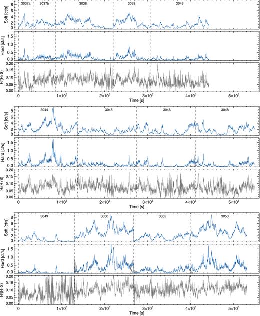
Concatenated EPIC-pn light curves from the 2016 observations, with their corresponding revolution number. The top panel shows the 0.3–1.2 keV (soft) band background-subtracted light curves (blue) and background light curves (grey). The middle panel shows the same for the 1.2–10 keV (hard) band. The bottom panel shows the hardness ratio H/(H + S). Revolution 3037 is split into two due to an observational gap.
The flux distributions using dt = 200 s for the soft (0.3–1.2 keV) band and hard (1.5–10.0 keV) band are shown in Fig. 2. We use 1.5–10.0 keV for the hard band to ensure we are not sampling the energy range dominated by the soft-band component. The log-transformed flux distribution is also shown in Fig. 2, which is expected to be Gaussian if the flux distribution is lognormal (see e.g. Edelson et al. 2014). For both bands a clear deviation from Gaussian is observed.
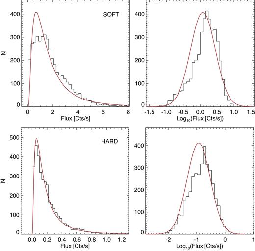
Flux distributions (left) and log-transformed flux distributions (right) for all 2 Ms data. The top panels show the 0.3–1.2 keV (soft) band and the bottom panels the 1.5–10.0 keV (hard) band. The red lines are the best-fitting lognormal model to the flux distributions and its subsequent log transform.
We fit the flux distributions with the two-parameter lognormal model using the r1 package fitdistrplus2 (Delignette-Muller & Dutang 2015), using the maximum likelihood estimation (MLE) method. The best-fitting models are shown in Fig. 2 (left) along with the log-transformed model (right). This model clearly gives a poor fit to the data in both bands. Fitting with the three-parameter lognormal distribution, which includes a counts offset parameter, produced negative values for the offset. This version of the model also gives a poor description of the log-transformed flux.
We use fitdistrplus to explore other types of distributions. A Cullen and Frey graph, which uses the skewness and kurtosis of the data (Cullen & Frey 1999), suggests a gamma or Weibull distribution provides a better description of the data. The Akaike information criterion (AIC; Akaike 1974), based on the log-likelihood function, was used to assess the model goodness of fit. Indeed, both the gamma and Weibull distributions produced a significantly lower AIC value than the lognormal. As the flux distributions of accreting systems typically show lognormal behaviour we just show that model, and its discrepancy with the data, here.
3.1 Stationarity of the data
The light curves of accreting sources are produced by a stochastic process. This process is considered stationary when the mean and variance tend to some well-defined value over long time-scales. Knowing whether this stochastic process is stationary is important for both connecting the observed variability properties to physical models of accretion (e.g. Cowperthwaite & Reynolds 2014; Hogg & Reynolds 2016) and using the variability to study the connection between different emission components (e.g. Uttley et al. 2014). AGNs are typically considered weakly non-stationary, as the low-frequency power spectral density (PSD) break is typically not observed: The low-frequency rollover to zero amplitude would provide a well-defined mean at some long finite duration. Typical observations in all wavebands capture the high-frequency part of the PSD, which is characterized by a red noise process, with P(f) ∝ f−α and α ≳ 2 (e.g. González-Martín & Vaughan 2012). The PSD flattens to α ∼ 1 below some high-frequency break.
All red noise processes show random fluctuations in both mean and variance, with the variance distributed in a non-Gaussian manner with large scatter. The changes in variance alone provide little insight as they are expected even when the underlying physical process is stationary: They are simply statistical fluctuations intrinsic to the stochastic process. See e.g Vaughan et al. (2003b) and Uttley et al. (2005) for more discussion on the stationarity of accreting systems.
These changes in the underlying variability process can be seen in Fig. 3, where the top panel shows the mean source flux in 5 ks time bins for the 2016 (∼1.5 Ms) observations. The middle panel shows the individual rms estimates for each 5 ks segment, computed by integrating the noise-subtracted power spectrum in each segment using dt = 20 s. This is roughly equivalent to Fourier frequencies in the range f = [0.2–25] × 10−3 Hz. The changes in rms can be seen to broadly track the changes in mean flux. The variable rms indicates genuine (strong) non-stationarity. However, this form of strong non-stationarity is to be expected as all accreting sources are observed to follow the linear rms–flux relation, where the mean flux in a time segment linearly correlates with the rms in that segment (e.g. Uttley & McHardy 2001; Uttley et al. 2005; Vaughan et al. 2011). If this can be cancelled out by dividing the rms values by the mean flux, then the rms–flux relation is the only source of (strong) non-stationarity (see Vaughan et al. 2003b).
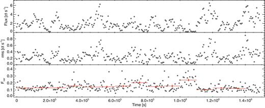
The running 5 ks count rate and variability amplitude measures for the 0.3–1.2 keV band. The top panel shows the mean flux and the middle panel shows the rms variability amplitude over the 5 ks bin. The grey points in the lower panel show the fractional variability amplitude (Fvar). The red bins are the mean of 20 consecutive Fvar estimates.
We can factor out the rms–flux relation by estimating the fractional variance (Fvar) of each segment (Vaughan et al. 2003b). This requires a large amount of data; at least N × M = 20 × 20 = 400 data points, where N is the number of time bins in a light-curve segment and M is the number of segments, are needed to produce a single well-determined estimate (Vaughan et al. 2003b). We therefore bin over 20 neighbouring points of Fvar, which is shown in the bottom panel of Fig. 3. The observations are clipped to integer lengths such that the average does not consist of bins from different observations. Errors are estimated using equation 11 of Vaughan et al. (2003b). We can test for changes in Fvar by fitting a constant model to the binned data, shown in red in Fig. 3. The fit gives χ2 = 33.1 for 12 degrees of freedom, with p = 0.0005.
We test for a constant Fvar on both longer and shorter time-scales. Using a segment length of 2 ks and the same dt = 20 s, equivalent to f = [0.5–25] × 10−3 Hz, the fit of a constant model gives χ2 = 106.7 for 36 degrees of freedom, with p < 10−8. Using a segment length of 10 ks and dt = 100 s, equivalent to frequencies f = [0.1–5] × 10−3 Hz, a constant model fit gives χ2 = 16.8 for 6 degrees of freedom, with p = 0.009. The 1.2−10.0 keV band also shows a similar deviation from constant Fvar.
After accounting for the effect of the rms–flux relation we are left with evidence for a further source of strong non-stationarity in the variability of IRAS 13224–3809. The non-stationarity of the data appears to be changing slowly. This can be seen in the running Fvar values in Fig. 3: Neighbouring points are consistent with each other, whereas a slow trend in Fvar is apparent over the length of the observing run, as well as larger deviations when the source is at low flux. This limits the minimum duration for which stationarity can be significantly detected given the current data quality: Neighbouring observations are approximately stationary. This is explored further using PSD analysis in Section 4, where non-stationarity manifests itself as PSD shape and/or normalization changes.
3.2 Rms–flux relation
Accreting black holes display larger amplitude variability when the mean source flux is higher (e.g. Lyutyi & Oknyanskii 1987; Uttley & McHardy 2001; Uttley et al. 2005; Vaughan et al. 2011). This can be seen for IRAS 13224–3809 if we look at the top two panels of Fig. 3, where the flux and rms track each other reasonably well. The relationship of flux and rms is observed to be linear in all accreting sources observed so far (e.g. Uttley & McHardy 2001; Uttley et al. 2017). The rms–flux relation was first tested in IRAS 13224–3809 using both ROSAT and ASCA data (Gaskell 2004). The data were found to be consistent with a linear relation.
We test the rms–flux effect in IRAS 13224–3809 by dividing the data into 5 ks continuous segments (with dt = 20 s) and computing the mean and rms, in each segment. Following Vaughan et al. (2011) and Heil et al. (2012), the rms is determined by computing a periodogram (in absolute units) for each segment and subtracting the Poisson noise level from each periodogram. The data were sorted on mean flux before grouping and averaging into several flux bins, Fi. The rms, σi, is then estimated by integrating the averaged power spectrum over the desired frequency range. The uncertainties on the rms estimates are computed from the variance of the individual χ2-distributed periodogram values (see Heil et al. 2012). We averaged over a minimum of 40 data points (typically >70) and checked for any negative variances in the averaged power spectra, of which there were none on the time-scales investigated.
The rms–flux relations for the [1–10] × 10−3 and [0.2–1] × 10−3 Hz soft band (0.3–1.2 keV) for all 2 Ms data are shown in Fig. 4 (left). These frequency ranges were chosen in order to maximize the number of data points forming Fi and σi. We fit the data with the linear model −σi = k(Fi–C), where C is a constant offset on the flux axis and k is the gradient. For both frequency bands we find a significant deviation from the linear model, with the best-fitting models having p < 10−4. The observed trend in the data is steeper at lower fluxes and flattens off with increasing flux. This is equivalent to the light curves being fractionally more variable at lower fluxes, as we found in Section 3.1.
![Left: the [1–10] × 10−3 and [0.2–1] × 10−3 Hz rms–flux relations for the 0.3–1.2 keV band using all 2 Ms data. The dotted line is the best-fitting linear model with the residuals shown in the middle panel: open symbols are the linear model. The solid red line is the best-fitting model $\sigma _i = C + N F_{i}^{1-\alpha ^{-1}}$, with α = 3, and the residuals are shown in the bottom panel. Right: the [1–10] × 10−3 and [0.5–5] × 10−3 Hz rms–flux relations for the 1.5–10.0 keV band.](https://oup.silverchair-cdn.com/oup/backfile/Content_public/Journal/mnras/482/2/10.1093_mnras_sty2527/2/m_sty2527fig4.jpeg?Expires=1749879920&Signature=NVFgrBrWnueohe8il1e3SmQtcLTyfeaeXx0wuboGEVA66kRlAsWZdicnl78ByTxa1Pst9rGO-pnLItZqIkcNY2fFSKcOfcY9VNlfEelHGB-9otKOJSoJkc6W1YdQiQaPdtpdP619M180LHmH1KtWWPPO5TiIP88lX0JqCdK~~P8muudSrrok8U7ZnhnWsSjx3hpTS476NDCljrJraXCUE1ChN8NLZV8xYp4LFqvp0YN2fD~qzv5B4eHlK-f-uxcSpWk1-XrBMB2QqHECSKSYjwXF7G2ngbir70W815H~wfpMpSDTiDigAwN-PaA2xrmv36~tasR~08OaYIEXJJf76g__&Key-Pair-Id=APKAIE5G5CRDK6RD3PGA)
Left: the [1–10] × 10−3 and [0.2–1] × 10−3 Hz rms–flux relations for the 0.3–1.2 keV band using all 2 Ms data. The dotted line is the best-fitting linear model with the residuals shown in the middle panel: open symbols are the linear model. The solid red line is the best-fitting model |$\sigma _i = C + N F_{i}^{1-\alpha ^{-1}}$|, with α = 3, and the residuals are shown in the bottom panel. Right: the [1–10] × 10−3 and [0.5–5] × 10−3 Hz rms–flux relations for the 1.5–10.0 keV band.
A linear rms–flux relation is a consequence of a lognormal transform of an underlying Gaussian process light curve (Uttley et al. 2005, Uttley et al. 2017). We test if some other transformation of an underlying Gaussian light curve, g(t), is producing the observed light curves x(t) in IRAS 13224–3809. For the case of a lognormal distribution, x(t) = exp[g(t)], following equation D1 in Uttley et al. 2005, the rms σx ∝ x(t), giving the linear relation commonly observed. For a PL transformation we have x(t) = g(t)α and therefore |$\sigma _{x} \propto x(t)^{1-\alpha ^{-1}}$|. We note here that this generalization is only strictly true for a low fractional rms (Uttley et al. 2005), which is ∼15 per cent in these frequency bands.
We fitted the rms–flux data with the model |$\sigma _i = C + N F_{i}^{\beta }$|, where β = 1 − α−1 and C is a constant rms offset. We initially allow N, C ,and β to be free parameters. A good fit to the data is found with values of β in the range 0.5–0.7. For illustrative purposes we show only the α = 3 (β = 2/3), with the parameters N and C free, model fit to both frequency ranges in Fig. 4. The residuals in the lower panel show how this model form provides a better description of the data over the linear. We note here that the model did not give an acceptable fit to the [0.5–5] × 10−3 Hz data, with p < 10−5 for any β. This is because of the large amount of scatter in the data, but the overall trend is consistent with the model. The PL model is preferred to the linear model at >5σ.
The 1.5–10.0 keV band [0.5–5] × 10−3 Hz rms–flux relation is shown in Fig. 4. The above linear model gives an acceptable fit with χ2 = 11.6 for 8 degrees of freedom, p = 0.17, in contrast with the same frequency range for the soft band in Fig. 4. However, we note the shape of the residuals is similar to the soft-band data. For higher frequencies ([1–10] × 10−3 Hz) a linear model also gives an acceptable fit, with p = 0.57. As we move to lower frequencies, the [0.2–1] × 10−3 Hz gives only a marginally acceptable fit, with p = 0.006 (∼3σ), suggesting we are starting to see a deviation from linear at this frequency.
We compute the rms–flux relation for the hard band on longer time-scales ([0.1–1] × 10−3 Hz) in Fig. 4 (blue). At this frequency band a clear deviation from the linear model is also found, with p = 0.0002. The blue solid curve in Fig. 4 shows the best fitting PL model with α = 3 (β = 2/3) and parameters N and C free. This model gives a better description of the data, with p = 0.3. We note that the soft-band rms–flux relation in this frequency range also displays the same deviation from the linear trend; however, we do not plot that here. The deviation from a linear rms–flux relation has a clear energy and frequency dependence in IRAS 13224–3809. In the hard band the deviation increases as we move to lower frequencies.
We show that this deviation from a linear relation can be seen in a subsection of the data. Fig. A1 shows the comparison between the 2011 and 2016 soft-band (0.3–1.2 keV) rms–flux relations, where the deviation from a linear model is apparent in both epochs. This tells us the non-linear relation is an intrinsic property of the source, rather than being caused by some outlying observations. As >40 data points are required for each flux bin we cannot examine the rms–flux relation on an orbit-by-orbit basis.
For comparison we show the 0.3–10.0 keV rms–flux relation for the NLS1 galaxy 1H 0707–495 in Fig. A2. The data are reduced in a similar manner as described in Section 2. This source shows similar power spectra, time lag, and spectral variability properties to IRAS 13224–3809 (e.g. González-Martín & Vaughan 2012; Kara et al. 2013; Done & Jin 2016) and has a comparable count rate and total XMM–Newton exposure, with ∼1.3 Ms for 1H 0707–495. A simple linear model gives an adequate fit to the data, with χ2 = 12.1 for 8 degrees of freedom and p = 0.1. This was the case for any energy band investigated for frequencies as low as 1 × 10⁻⁴ Hz. We note here the clustering of flux points in Fig. A2 around ∼3 count s−1 and fewer points at lower fluxes compared to the flux sampling of IRAS 13224–3809. In addition, we also repeat the analysis from Section 3.1 on 1H 0707–495 and find a constant model gives an acceptable fit to the Fvar time series.
4 POWER SPECTRAL DENSITY
The results in Section 3 provide significant evidence for strong non-stationary variability in IRAS 13224–3809 . We can see if this also manifests itself in the power spectrum (PSD). The PSD was estimated using standard methods (e.g Bartlett 1948; van der Klis 1989). We first estimate the periodogram in each segment before averaging over M segments at each Fourier frequency, followed by averaging over N neighbouring frequency bins. The number of estimates at each PSD bin, n = M × N, should be >20 to give error bars that are Gaussian distributed (Papadakis & Lawrence 1993; Vaughan et al. 2003b). If the PSD is stationary (or at most weakly non-stationary), we expect to see no significant change in shape or normalization when computed with a fractional rms normalization.
Like any other time series analysis method, detecting significant non-stationarity in the PSD gets progressively harder as the total light-curve duration of each individual PSD decreases: Larger error bars make detecting smaller changes difficult. To see if the PSD is changing shape (or normalization) over time, we split the data into seven epochs, each formed from light curves from 2−3 consecutive XMM–Newton observations. We divide the data into segment lengths of 60 ks and linearly bin over at least 4 neighbouring frequency bins. This allows us to measure a PSD down to low frequencies with reasonable frequency resolution, whilst still satisfying the requirement for at least 20 averages per frequency estimate. We make use of the 2011 and 2016 observations only, as the 2002 observation is too short and too separated in time. The epoch-resolved PSDs are formed from Revs 2126, 2127 (epoch 1); 2129, 2131 (epoch 2); 3037, 3038, 3039 (epoch 3); 3043, 3044 (epoch 4); 3045, 3046 (epoch 5); 3048, 3049 (epoch 6); and 3050, 3052, 3053 (epoch 7).
Fig. 5 shows the rms-normalized, epoch-resolved PSDs for the 0.3–1.2 keV band. The PSDs are Poisson-noise subtracted using standard formulae (Vaughan et al. 2003b) and clipped at ∼2 × 10⁻³ Hz, above which the noise dominates. The solid line shows the best-fitting simple PL model (see equation 1) to the epoch 1 PSD, with normalization N = 4.65 ± 0.17 × 10⁻⁶ and α = 1.92 ± 0.06. The lower panel shows the ratio of each epoch PSD to the best-fitting PL to epoch 1. The PSDs qualitatively appear to be well described by two peaked components: one at ∼5 × 10⁻⁵ Hz and another at ∼10−3 Hz. A clear change in PSD normalization is apparent as well as smaller change in PSD shape, i.e. shift in peak frequency, of the low-frequency component.

The soft (0.3–1.2 keV) band epoch-resolved, Poisson-noise-subtracted PSDs with rms normalization. The data are colour coded by mean source flux, with darker shades of red representing higher source flux light-curve segments. The bottom panel shows the ratio to the best-fitting PL model to the epoch 1 PSD.
The PSDs are colour coded by mean source flux of the light curves used to form each one. The change in PSD shape correlates extremely well with change in mean source flux, with epochs with lower source flux having systematically higher normalization, in agreement with the results from Sections 3.1 and 3.2. The trend isn’t perfect with source flux; however, this appears to be the dominant factor in the change in PSD shape and normalization. The changes in the underlying broad-band PSD model components are explored in Section 4.1. We show the same plot for the 1.2–10.0 keV band in Fig. A3, which displays the same PSD shape change with epoch and flux. Investigating the changes in PSD shape on shorter time-scales, equivalent to searching shorter time-scales over which the non-stationarity is occurring, is of course possible. However, we lose low-frequency information as well as PSD resolution (having to bin over more adjacent frequencies). We repeated the PSD analysis using 30 ks segments formed from individual orbits only. This results in a similar change in PSD shape with the source flux being the dominant factor in PSD shape and normalization.
4.1 Modelling the PSD
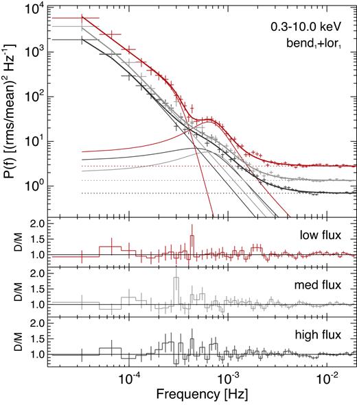
We start by modelling the 0.3–10.0 keV (total) PSD for all 2 Ms data, which is shown in Fig. 6. The results from previous sections show that the light curves are non-stationary. Strictly speaking, inferences from some time series analysis methods may be complicated when averaging light-curve sections that are known to be non-stationary. However, as we have seen in Fig. 5, the changes with epoch (flux) are dominated by normalization changes of two peaked components. We therefore first explore the average 2 Ms PSD in order to explore the nature of the broad-band components with the highest frequency resolution down to the lowest frequencies. We then go on to explore how these components change with epoch and flux.
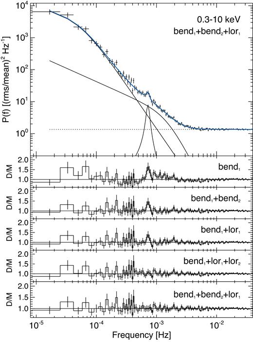
The 0.3–10.0 keV PSD using all 2 Ms data. The PSD is modelled using a combination of simple models, including a bending PL (bend) and Lorentzian (lor), described in detail in Section 4.1. The model shown is the best-fitting model (bend1 + bend2 + lor1), with bend frequencies νb1 ∼ 5 × 10⁻⁵ Hz, νb2 ∼ 1 × 10⁻³ Hz and Lorentzian centroid νc = 7 × 10⁻⁴ Hz.
We initially explore the model fitting in xspec using standard min χ2 methods. The quoted error bars represent the 90 per cent confidence levels. The curvature in the PSD means a model using only a single PL provides a bad fit, with χ2 = 419/134 degrees of freedom. We replace this with a single bending PL (bend), which with all parameters free gives a fit statistic χ2 = 201/132 degrees of freedom. The residuals of this model are shown in Fig. 6, where curvature at both low and high frequencies is seen. Fixing the low-frequency slope parameter αlow = 1.1 worsens the fit, with χ2 = 256/133 degrees of freedom. The curvature in the (bend) model residuals suggests the presence of a bend in the PSD at ∼a few × 10−5 Hz and an additional component at ∼10−3 Hz. We combine a PL with a bending PL (bend + PL) in order to model the additional component at high frequencies; however, this model is disfavoured with χ2 = 255/130 degrees of freedom. A model based on a simple power law plus a Lorentzian (pl + lor) also gives an unacceptable fit to the data, with χ2 = 327/131 degrees of freedom.
We next combine two bending power laws (bend1 + bend2), with all parameters free to vary. We initially set νb,1 = 2 × 10⁻⁵ Hz and νb,2 = 1 × 10⁻³ Hz, where the subscripts ‘1’ and ‘2’ refer to the first and second bend components, respectively. This model gives a vast improvement to the fit, with χ2 = 154.5/128 degrees of freedom. This corresponds to a Δχ2 = 46.5 for 4 degrees of freedom compared to the (bend) model, which is a >5σ requirement for an additional high-frequency component in the PSD. The model residuals are shown in Fig. 6. A significant bend frequency is detected in both components with best-fitting parameters νb,1 = 5.2 ± 0.4 × 10⁻⁵ Hz and νb,2 = 1.5 ± 0.4 × 10⁻³ Hz. Both low-frequency slopes gave values <1, with αlow,1 = 0.58 ± 0.38 and αlow,2 = 0.58 ± 0.38. Fixing either or both of these parameters to <1 did not add any significant improvement to the fit. We explore the best-fitting parameters in more detail further on.
The PSD clearly requires a component with curvature around 10−3 Hz. We therefore replace the second bend component with a Lorentzian to form the model (bend1 + lor1), to see if this adds any improvement to the modelling. The model provides the fit χ2 = 164/129 degrees of freedom, corresponding to a Δχ2 = 37 for 3 degrees of freedom compared to the (bend) model, which is also a >5σ improvement; however, this model provides a worse fit than the (bend1 + bend2) model. The model residuals are shown in Fig. 6. The bend parameters are consistent with the first bend component in the (bend1 + bend2) model. The best-fitting model has Lorentzian centroid νc = 6.1 ± 0.6 × 10⁻⁴ Hz and width σ = 5.1 ± 0.9 × 10⁻⁴ Hz. Lorentzian components in the PSDs of accreting sources are typically described in terms of their quality factor, Q = ν/Δν, where Δν is the FWHM of the profile (= σl in our case). For the (bend1 + lor1) model we find Q ∼ 1. Lorentzians with Q < 1 are typically considered broad-band noise components (e.g. Belloni 2010). This is unsurprising given a broad (in frequency) bending power-law component also describes the data well at high frequencies.
Narrow structure in the residuals of both the (bend1 + bend2) and (bend1 + lor1) models can be seen at ∼7 × 10⁻⁴ Hz in Fig. 6. We add an additional Lorentzian component to both the model variants with initial parameters νc = 7 × 10⁻⁴ Hz and σl = 1 × 10⁻⁴ Hz (Q = 7). The (bend1 + lor1 + lor2) model gave χ2 = 152.8/126 degrees of freedom, giving a Δχ2 = 11.2 for 3 additional parameters compared to the (bend1 + lor1) model. The model residuals are shown in Fig. 6.
The (bend1 + bend2 +lor1) model gave an adequate fit, with χ2 = 137.6/125 degrees of freedom. As this is the minimum χ2 found in the model fitting we show this model fit to the data and its residuals in Fig. 6. Compared to the (bend1 + bend2) model, this is an improvement of Δχ2 = 16.9 for 3 additional parameters. This roughly corresponds to a ≳ 3σ requirement of the narrow feature; however, see Section 4.4 for a detailed investigation of the significance of this feature. The Lorentzian component has Q ∼ 8 and an integrated rms amplitude of ∼3 per cent.
The model fitting for the (bend1 + bend2 + lor1) and (bend1 + lor1 + lor2) models was repeated using a Bayesian scheme, treating the log-likelihood function as ∼(−χ2/2). Simple uniform prior distributions were assigned to the parameters. We explore the posterior distribution of the parameters using a Markov Chain Monte Carlo (MCMC) scheme to randomly draw sets of parameters. We make use of the Goodman & Weare affine-invariant MCMC ensemble sampler, with the python module emcee3 (Foreman-Mackey et al. 2013), which is implemented in xspec through xspec_emcee.4 We generated 5 chains of length 50 000 after a burn-in period of equal length and checked for convergence using the Gelman–Rubin test (e.g. Gelman et al. 2003).
No parameter degeneracy was found for either the (bend1 + bend2 + lor1) or (bend1 + lor1 + lor2) models. The posterior parameter modes were in agreement with those found from the min χ2 method. As this gave the best fit, the parameter modes and 90 per cent credible intervals for the (bend1 + bend2 + lor1) model are shown in Table 1. In both models we detect a clear low-frequency bend with the low-frequency slope, αlow,1, significantly less than 1. In Fig. 7 we show the posterior distributions from the MCMC draws for the parameters αlow,1, νb,1, and αhigh,1 of the (bend1 + bend2 + lor1) model. The posterior distributions are clearly well sampled and show how a component with a break to low frequencies is required by the data.
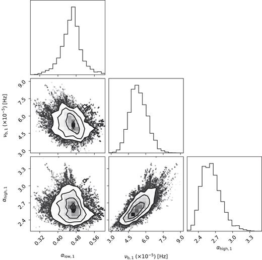
Posterior parameter distributions from the MCMC draws for the low-frequency bend component in the (bend1 + bend2 + lor1) model. The low-frequency slope αlow,1, bend-frequency νb1, and high-frequency slope αhigh,1 are shown.
Parameter values for the (bend1 + bend2 + lor1) model. The errors on the model parameters represent the 90 per cent credible intervals from the MCMC draws.
| En | αlow,1 | νb,1 | αhigh,1 | Nb,1 | αlow,2 | νb,2 | αhigh,2 | Nb,2 | νc | σl | Nl | PN | Apsd,1 | Apsd,2 |
|---|---|---|---|---|---|---|---|---|---|---|---|---|---|---|
| [keV] | [Hz] | [Hz] | [Hz] | [Hz] | [Hz] | |||||||||
| (×10−5) | (×10−3) | (×10−2) | (×10−4) | (×10−5) | (×10−3) | (×10−1) | (×10−3) | |||||||
| (1) | (2) | (3) | (4) | (5) | (6) | (7) | (8) | (9) | (10) | (11) | (12) | (13) | (14) | (15) |
| 0.3−10.0 | |$0.47_{-0.09}^{+0.07}$| | |$5.2_{-0.1}^{+0.1}$| | |$2.68_{-0.28}^{+0.32}$| | |$40_{-10}^{+30}$| | |$0.75_{-0.36}^{+0.21}$| | |$1.8_{-0.9}^{+1.2}$| | |$3.7_{-0.57}^{+0.62}$| | |$2.0_{-0.9}^{+0.8}$| | |$7.2_{-0.1}^{+0.1}$| | |$8.5_{-0.3}^{+0.4}$| | |$1.1_{-0.4}^{+0.4}$| | |$1.34_{-0.01}^{+0.01}$| | 1.1 ± 0.5 | 1.9 ± 0.6 |
| 0.3−0.7 | |$0.09_{-0.05}^{+0.04}$| | |$4.1_{-0.2}^{+0.2}$| | |$2.51_{-0.21}^{+0.42}$| | |$2.4_{-0.2}^{+0.2}$| | |$1.06_{-0.24}^{+0.19}$| | |$1.7_{-0.5}^{+0.7}$| | |$4.1_{-1.1}^{+3.2}$| | |$1.1_{-0.3}^{+2.1}$| | |$7.2_{-0.2}^{+0.1}$| | |$8.5_{-0.3}^{+0.4}$| | |$0.9_{-0.3}^{+0.3}$| | |$1.92_{-0.02}^{+0.02}$| | 1.2 ± 0.7 | 2.5 ± 1.1 |
| 0.7−1.2 | |$0.34_{-0.05}^{+0.03}$| | |$5.0_{-0.2}^{+0.2}$| | |$2.71_{-0.30}^{+0.52}$| | |$179.8_{-0.2}^{+0.2}$| | |$1.10_{-0.24}^{+0.15}$| | |$2.4_{-0.4}^{+0.4}$| | |$5.2_{-1.9}^{+1.7}$| | |$2.2_{-1.0}^{+2.2}$| | – | – | |$2.0_{-0.7}^{+0.7}$| | |$5.7_{-0.1}^{+0.1}$| | 1.3 ± 0.7 | 20.1 ± 11.8 |
| 1.2−3.0 | |$0.81_{-0.04}^{+0.05}$| | |$12.3_{-3.7}^{+4.1}$| | |$2.65_{-0.36}^{+0.82}$| | |$1.3_{-3.1}^{+2.9}$| | |$0.56_{-0.11}^{+0.11}$| | |$1.2_{-0.3}^{+0.3}$| | |$3.5_{-0.5}^{+1.1}$| | |$0.9_{-0.3}^{+0.3}$| | – | – | |$1.0_{-1.0}^{+0.5}$| | |$21.4_{-0.2}^{+0.1}$| | 1.2 ± 0.7 | 23.4 ± 13.7 |
| 3.0−10.0 | |$0.58_{-0.06}^{+0.04}$| | |$11.9_{-4.3}^{+5.2}$| | |$2.24_{-0.29}^{+1.02}$| | |$7.0_{-0.2}^{+0.2}$| | |$0.56_{-0.38}^{+0.22}$| | |$1.0_{-0.6}^{+0.9}$| | |$2.9_{-0.9}^{+1.2}$| | |$0.85_{-0.13}^{+1.9}$| | – | – | |$1.9_{-1.9}^{+2.2}$| | |$94.4_{-0.2}^{+0.1}$| | 0.4 ± 0.2 | 20.3 ± 11.9 |
Motivated by the low-frequency break, we replace the bend components with a Lorentzian to form the model (lor1 + lor2 + lor3). However, this does not provide any improvement to the fit, with χ2 = 164/126 degrees of freedom. We note the MCMC parameter sampling was performed on all simpler models described above, in order to fully sample the parameter space and ensure the best-fitting solution has been found. We also note that in all models described above there was a series of narrow residuals between ∼2 and 4 × 10⁻⁴ Hz, as can be seen in Fig. 6. Neither a broad nor narrow additional component to any of the models described above could account for these features.
AGN PSDs are susceptible to the effect of red noise leakage, where power from below the observing window function shifts to higher frequencies. If the power spectrum is steep (α ≳ 2 at or below the lowest observed frequency), significant distortion of the power spectrum will occur, and the slope will flatten towards α = 2 (see e.g. Uttley et al. 2002). As we detect a measurable bend and rollover (i.e. there is no increase in power outside our window) we estimate this effect to be minimal in our PSD (see also the long-term PSD in Section 4.5). At the highest frequencies, aliasing of power can add a frequency-independent level to the PSD. This effect will be minimal as we use contiguous light-curve time bins.
4.2 Energy dependence of the power spectrum
The energy dependence of the PSD was investigated by dividing the data into four broad energy bands – 0.3–0.7, 0.7−1.2, 1.2−3.0, and 3.0–10.0 keV – which are shown in Fig. 8. The PSDs show similar shape to the total band in Fig. 6. The narrow feature at ∼7 × 10⁻⁴ Hz is more apparent in the softer (0.3–0.7 and 0.7 − 1.2 keV) bands. Below ∼10−4 Hz the power is visibly weaker in the 3.0–10.0 keV band.

The energy-resolved PSD using all 2 Ms data. The model shown is the best-fitting model (bend1 + bend2 +lor1), with bend frequencies νb1 ∼ 5 × 10⁻⁵ Hz, νb2 ∼ 1 × 10⁻³ Hz and Lorentzian centroid νc = 7 × 10⁻⁴ Hz.
We model the PSDs with the two best-fitting models (bend1 + bend2 + lor1) from Section 4.1, starting with the min χ2 method. All parameters are initially free to vary, with the exception of the (lor) component νc and σl, which are tied across energy. The best-fitting (bend1 + bend2 + lor1) model provides a poor fit, with χ2 = 982/510 degrees of freedom. Allowing νc and σl free to vary provided minimal improvement to the fit. As outlined above, we explore the posterior parameter distributions using the MCMC scheme. The best-fitting model parameters are shown in Table 1. No degeneracies are found in the parameter distributions. In agreement with the min χ2 method, the normalizations of the lor components in the harder bands (1.2−3.0 and 3.0–10.0 keV) are consistent with zero, suggesting an energy dependence for this component. The marginal posterior distributions for the bend frequency, νb,1, are shown in Fig. 10. We detect a clear change in bend frequency with energy at >99.7 per cent confidence, with νb,1 increasing with energy. The softer bands favour values of ∼5 × 10⁻⁵ Hz, whilst the harder bands are consistent with ∼1 × 10⁻⁴ Hz.
The bend2 component also shows evidence for an energy dependence (see Table 1). The lower panel in Fig. 10 shows the marginal posterior distributions for νb,2, which shows a decrease in energy. The bend2 parameter αlow,2 decreases with energy and αhigh,2 increases with energy. The model with αlow,2 and αhigh,2 tied across all energy bands also resulted in a significant decrease in νb,2 with energy.
The energy-dependent PSD was explored using the (bend1 + bend2 + lor1) model, which also gave a poor fit with χ2 = 987/510 degrees of freedom. Consistent values with the previous model were found for the model peak parameters, with the lor centroid frequency, σl, also decreasing with increasing energy band.
Despite the poor fit of both models to the data, no coherent broad (in frequency) structure is seen in the residuals in Fig. 8. A number of very narrow residuals confined to ∼1−2 frequency bins are present, which do not appear to have any consistent energy dependence. Adding progressively more Lorentzian components to model the narrow structure does not significantly improve the fit. We confirm that these narrow features are not a result of the geometrical frequency binning, as they are also present in the unbinned PSD. We check that the single-component (bend) model cannot fit the 1.2−3.0 and 3.0–10.0 keV bands individually. This model gave a poor fit to both data, with χ2 = 321/132 degrees of freedom and χ2 = 231/132 degrees of freedom, respectively.
4.3 Flux-dependent power spectrum
The epoch-resolved PSDs in Section 4 showed the PSD changes in normalization over time, with the changes dominated by the source flux. We explore the flux dependence of the 0.3–10.0 keV PSD. Any changes in the shape of the variability components in the PSD with source flux may give some insight into the origin of the non-stationarity in the light curves. We divide the data into three flux bins, containing roughly a third of the data each. In this way, we can achieve better signal-to-noise and frequency resolution compared to using the seven epoch-resolved PSDs. The PSDs are shown in Fig. 9, where a change in the normalization and curvature of the spectrum is apparent.
The flux-resolved 0.3–10.0 keV PSD using all 2 Ms data. The model shown is the (bend1 + lor1).
We start with our two-component models from Section 4.1. As before we use MCMC chains to explore the marginal posterior densities. The (bend1 + bend2) model gave an acceptable fit, with χ2 = 198.6/153 degrees of freedom. The (bend1 + lor1) model gave some improvement, with χ2 = 168.2/156 degrees of freedom. This best-fitting model is shown in Fig. 9. We detect a clear change in the low-frequency bend, νb,1, which can be seen in posterior distributions in Fig. 10(c). We also plot the posterior distributions for the Lorentzian centroid, νc, in panel (d). The high- and low-flux data show a change in νc at around 90 per cent significance. The results were consistent when the Lorentzian width, σl, was tied across flux.
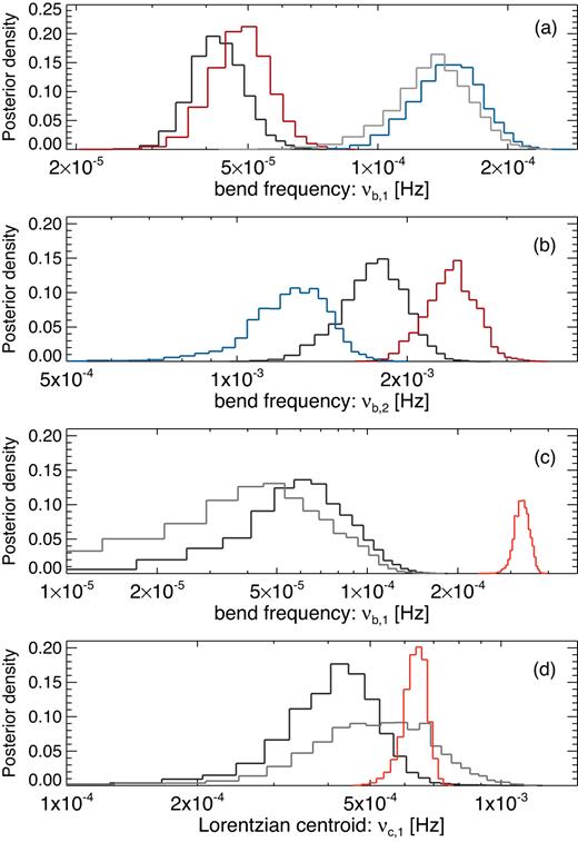
Marginal posterior probability density for model parameters computed using MCMC draws. Panel (a) shows the bend frequency, νb,1, in the (bend1 + bend2 + lor1) model. The colours represent the same energy bands used in Fig. 8. Panel (b) shows the same for νb,2. Panel (c) shows the flux dependence of νb,1 in the (bend1 + lor1) model, with the same colours shown in Fig. 9. Panel (d) shows the same for the Lorentzian centroid, νl,1.
The bend1 component at 3 × 10⁻⁴ Hz in the low-flux PSD has different slope values from those found for the same component in all previous modelling. Rather than an extreme change in this component producing the resulting low-flux PSD, we test to see if an additional component is increasing in normalization as the flux drops. We add a broad Lorentzian to form the model (bend1 + lor1 +lor2), with the lor2 component initially set to 3 × 10⁻⁴ Hz. This model gives χ2 = 168.1/153 degrees of freedom. The bend1 component has consistent parameters across flux, whilst the lor2 component is not required by the high- and medium-flux data. Regardless of what component is used to model the bend seen in the low-flux data, a clear change in the shape of the PSD is seen with source flux.
Adding a an additional narrow Lorentzian component is not required by the data in either model. However, we note the high-flux PSDs have residuals around 7 × 10⁻⁴ Hz. We also note residuals around 2 × 10⁻³ Hz in the low-flux data, which also showed no significant requirement for an additional Lorentzian component.
The energy- and flux-resolved PSDs for the 0.3–1.2 and 1.5–10.0 keV bands showed a similar trend to the total band PSD: The low-frequency break moved to higher frequencies in the lowest flux segments. The changes in the epoch-resolved PSDs are consistent with the changes found in source flux, as can be seen in Fig. 5.
4.4 Significance of narrow Lorentzian
In Section 4.1 we found strong evidence for an additional narrow Lorentzian component at 7 × 10⁻⁴ Hz in the PSD. The detection of additional narrow components in power spectra suffers from the same statistical problems as fitting lines to energy spectra (see e.g. Protassov et al. 2002; Vaughan 2010; Vaughan et al. 2011 for further discussion on these issues). To mitigate these issues, the critical value of a test statistic, Tcrit, was explored using MCMC simulations in order to determine the false alarm probability. We follow the method outlined in Vaughan et al. (2011, Appendix B), where Tcrit is closely related to the likelihood ratio test. From the MCMC simulations of the total band (bend1 + bend2) model, we have Tcrit = 14.2 for probability α = 0.0027. This tells us that a reduction in χ2 > 14.2 will occur by chance with probability α = 0.0027. Our measured value of T from Section 4.1 is 16.9, so the posterior predictive p-value of the feature is <0.0027 (i.e >3σ).
We search for significant outliers in the periodogram of each individual observation using the Bayesian maximum-likelihood method of Vaughan (2010; see also González-Martín & Vaughan 2012; Alston et al. 2014b; Alston et al. 2015), using the (bend1 + bend2) continuum model described above. Using a criterion of p < 0.01 as the detection threshold, we detect no significant outliers in any individual periodogram. This suggests the narrow feature we detected in the binned PSD is on the threshold for detection within an individual observation, and is only detected due to the large amount of data being averaged in the binned PSD.
4.5 Long-term power spectrum
In order to determine whether we are sampling a broad range of the underlying PSD, and to have a better understanding of the bend frequency, we next look at the power spectrum of the long-term light curve. The spacing of the 2016 observations over an ∼1 month period (with more ‘on’ times than there are gaps) allows us to investigate the shape of the long-term PSD. We use the continuous-time autoregressive moving average (CARMA) modelling method described in Kelly et al. (2014) using the publicly available code carma_pack.5 The method can handle data gaps, allowing us to determine the PSD down to the frequency equivalent to the time-scale of the total observation campaign (∼30 d; ∼3 × 10⁻⁷ Hz). The CARMA method assumes the light-curve results from a Gaussian process and estimates the model power spectrum as the sum of multiple Lorentzian components. The method uses an MCMC sampler to build up Bayesian posterior summaries on the Lorentzian function parameters. We used a bin size dt = 200 s in this analysis to reduce the computational expense, giving a total number of bins Nbins = 7616.
We considered CARMA(p, q) models, where p is the number of autoregressive coefficients and q is the number of moving average coefficients, and q < p for a stationary process (see Kelly et al. 2014 for more details). The corrected Akaike information criterion (AICc; Hurvich & Tsai 1989) was used to choose the values of p and q, for all q < p with pmax = 7 (see equation 34 in Kelly et al. 2014). This penalizes progressively more complex models if they do not produce a better improvement in the log-likelihood.
We first use the 0.3–10.0 keV light curve that minimized the AICc for the CARMA(3,2) model. The resulting model power spectrum is shown in Fig. 11 [note the f × P(f) units]. The confidence intervals represent the uncertainty in the Lorentzian components formed from the CARMA coefficients. Two clear bends can be seen in the data: a low-frequency bend at ∼10−5 Hz and a higher frequency bend at ∼10−3 Hz, consistent with the short-term PSD fitting in Section 4.1. The low-frequency slope clearly has α < 1.
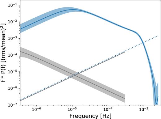
Long-term power spectrum from the CARMA(3,2) modelling for the 0.3–10.0 keV band (blue), in units of frequency × power. The estimate of the power spectrum is given by the solid line, the 95 per cent confidence intervals are given by the shaded region, and the dotted line shows the Poisson noise level. The optical power spectrum from the CARMA(2,0) modelling is shown in grey, with the Poisson noise level given by the solid grey line.
Models with lower values of p all produced a low-frequency bend at ∼10−5 Hz, with the lowest frequency slope α < 1. The effect of increasing p was to model the curvature around ∼10−3 Hz. p > 3 did not produce significantly different power spectra, but did increase the confidence intervals at high frequencies.
In Sections 3 and 4 we found evidence for significant non-stationary variability in the light curve of IRAS 13224–3809. In its current implementation, carma_pack cannot handle q ≥ p for non-stationary processes. However, we use the method to give some indication of the components that form the broad-band PSD. In addition, the output of CARMA can be used as an additional check for stationarity. If the light curve is formed from a Gaussian process, then the standardized residuals of each MCMC light curve draw will follow a standard normal distribution (Kelly et al. 2014). In Fig. A4 we show the output of the MCMC run for the CARMA(3,2) model. The overlaid standard normal distribution is a bad match to the data, suggesting an underlying Gaussian process is a bad assumption for the variability in IRAS 13224–3809. This provides further evidence for non-stationarity variability in this source.
We next look at the energy dependence of the long-term power spectrum, using two bands: soft (0.3–1.2 keV) and hard (1.5–10 keV). The best-fitting CARMA power spectra estimates are shown in Fig. 12. The soft band showed a minimum AICc for the CARMA(3,2) model. The hard band also minimized the AICc for the (3,2) model, and is also shown in Fig 12. The error bars and difference between the soft- and hard-band PSDs are consistent with those derived from Fourier methods in Section 4.2. Both energy bands have a similar divergent low-frequency slope below a bend frequency ∼10−5 Hz. Further evidence is seen for an energy-dependent low-frequency bend. The high-frequency slope is flatter in the hard band, in agreement with the PSD modelling in Section 4.1.
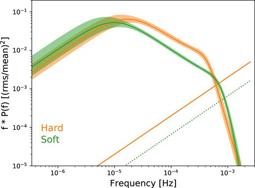
Long-term power spectrum from the CARMA(3,2) modelling of the soft (0.3–1.2 keV; green) and hard (1.5–10 keV; orange) bands in units of frequency × power. The estimate of the power spectrum is given by the solid line and the 95 per cent confidence intervals given by the shaded region. The dotted green line shows the Poisson noise level for the soft band and the solid orange line is that of the hard band.
The Optical Monitor (OM) onboard XMM–Newton means we can also study the optical power spectrum on long time-scales. The data were taken in the UVW1 filter and have a mean exposure bin of 2700 s, giving Nbins = 524 (see Buisson et al. 2018 for details on the data reduction). The CARMA(2,0) model minimized the AIC and the power spectrum estimate is shown in grey in Fig. 11. The optical PSD shows no significant bend for this or any more complex model variant. This agrees with Buisson et al. (2018), where a simple power law was found to describe the PSD above ∼10−5 Hz. The lack of any features in the optical PSD tells us the low-frequency bend at ∼10−5 Hz in the X-ray bands is not a result of the sampling pattern of the observations. To measure the PSD down to even lower frequencies we perform the CARMA analysis on the long-term Swift 0.3–10.0 keV light curve, spanning 6 yr. The resulting plot is shown in Fig. A5, where this time we show the 99 per cent confidence intervals. No additional components are observed down to frequencies ∼5 × 10⁻⁹ Hz.
5 DISCUSSION
5.1 Summary of results
We have presented a detailed analysis of the variability properties of one of the most variable NLS1 galaxies, IRAS 13224–3809. We have used the longest XMM–Newton observation to date on a single AGN, combing a recent 1.5 Ms VLP observation and 500 ks of archival data. We briefly summarize the main results here before discussing them in the context of accreting black holes.
The distribution of flux in both soft and hard energy bands shows a clear deviation from a lognormal distribution, which is typically observed in accreting sources. The majority of the discrepancy comes at lower source flux.
The long-term changes in fractional variance tell us that the rms–flux relation is not the only source of strong non-stationarity in the light curves. The strong non-stationarity is also observed in the PSD: small, but significant, changes in the broad-band PSD shape and normalization from different epochs of the data.
We show for the first time a non-linear rms–flux relation for any accreting compact object. It is well described as rms ∝ flux2/3, meaning the source is fractionally more variable at lower source flux. This is seen on time-scales ∼10−4–10−2 Hz in the soft band, but only below 10−3 Hz in the hard band.
Multiple peaked components are required to model the power spectrum: a broad component peaking at ∼103 Hz and one at ∼5 × 10⁵ Hz. The low-frequency break has slope α < 1 down to low frequencies. An energy dependence is seen in the low-frequency break, with νb increasing with energy.
The non-stationarity is observed in the epoch- and flux-resolved PSD: the low-frequency break, νb, increases in frequency as the source flux drops. In addition, we find weak evidence for the high-frequency break increasing in frequency with decreasing flux.
A narrow Lorentzian feature is detected in the PSD at 7 × 10⁻⁴ Hz. The line is only detected below 1.2 keV and has Q ∼ 8 and rms = 3 per cent.
CARMA analysis of the long-term light curve also reveals the low-frequency break to zero power below ∼10−5 Hz in all energy bands. This is the second time such a low-frequency rollover in the PSD has been observed in any waveband in an AGN.
5.2 Stationarity
The Fvar and PSD analysis reveal strong non-stationarity in the light curves of IRAS 13224–3809. In terms of PSD components, the non-stationarity can be explained in terms of two broad peaked components changing in normalization. These components change over time in a way that is linked with mean source flux. The PSD could be changing on faster time-scales than we have shown using the epoch-resolved approach (≲ day). However, we have reached the limit of what can be statistically resolved with current data quality, using standard methods. The PSD can therefore be considered approximately stationary on ≲ days time-scales. In this way it is no different to other AGNs, where PSDs compared over longer epochs are approximately consistent with each other. The fact that the PSDs from epoch to epoch have similar shape tells us that within each epoch the shape of the variability components can’t be varying dramatically.
The following discussion is based on the idea that the PSD is formed of two broad peaked components that vary in time with mean source flux. However we caution the reader that inferences made from these data may be complicated by changes occurring on time-scales faster than can be measured using standard techniques.
The rollover in the low-frequency slope means the PSD is not divergent. This is typically not observed in AGNs, which are therefore considered weakly non-stationary. This is unsurprising given that long-term light curves (∼14 yr) do not show large changes in source flux: The mean 0.3–10.0 keV band count rate of the 2002 and 2011 observations is almost identical to the 2016 observations. It may well be that CARMA analysis is not the best way to measure a non-stationary PSD. However, the CARMA PSDs are consistent with the shape of those from the direct PSD fitting, even if the component normalizations do change over time. The CARMA method is currently the best approach for modelling the long-term PSD. We will develop this method further for non-stationary data in a future paper.
5.3 Black hole mass and accretion rate
The black hole mass of IRAS 13224–3809 is uncertain, with current estimates in the range |${M_{\rm {BH}}}\sim 10^{6-8}$| (Czerny et al. 2001; Bian & Zhao 2003; Sani et al. 2010), with none of these estimates coming from reverberation mapping.
This scaling relation was recently updated using a larger sample of detections of bend frequencies in the PSD by González-Martín & Vaughan (2012), with parameters A = 1.34, B = −0.24, and C = −1.88. Using νb,2 = 1.8 × 10⁻³ Hz, we determine a lower value of |${M_{\rm {BH}}}\sim 0.5 \times 10^6 {\, \mathrm{M}_{\odot }}$|. Our BH mass estimate for IRAS 13224–3809 is therefore |${M_{\rm {BH}}}= [0.5{--}2] \times 10^6 {\, \mathrm{M}_{\odot }}$|.
As we detect two clear breaks in the PSD this means we have to decide which to use in the BH mass estimate. The CARMA modelling of the long-term PSD shows we are sampling the low-frequency rollover in this source. It is therefore most likely that the high-frequency bend is the analogue of the break frequencies detected in other sources. The NLS1 galaxy Ark 564 is the only other source with a well-defined low-frequency break in the PSD (McHardy et al. 2007). The BH mass in Ark 564 is well determined from reverberation mapping. Indeed, McHardy et al. (2007) found the high-frequency break time-scale in this source to be consistent with the mass−Tb relation.
We use the new BH mass estimate to update the estimate of the accretion rate. In terms of Eddington fraction, this currently has estimates of |${\dot{m}_{\rm Edd}}\gtrsim 0.3{--}10$| (Buisson et al. 2018). Using the bolometric luminosity above, we derive the accretion rate in terms of the Eddington fraction, |${\dot{m}_{\rm Edd}}\gtrsim 1-3$|. It is therefore highly likely that IRAS 13224–3809 is accreting at or around the Eddington limit.
The BH mass–TB relation predicts the accretion rate to scale inversely with the break time-scale, as |$T_{\rm b} \approx {M_{\rm {BH}}}^{1.15} / {\dot{m}_{\rm Edd}}^{0.98}$| (McHardy et al. 2006). The flux-dependent PSD modelling in Section 4.3 shows tentative evidence for an anticorrelation in the high-frequency bend, νb,2, with source flux: The centroid frequency changes by ∼50 per cent. This change in the break time-scale is at odds with the McHardy et al. (2006) relation, as we see a higher break frequency at lower source flux (lower accretion rate). If the break time-scale scales with the thermal or viscous time-scale, then it is expected that the inner edge of the accretion disc, Rin, scales inversely with the accretion rate. We may therefore be seeing the opposite effect in IRAS 13224–3809, which may be related to the above Eddington rate in this source. Tentative disagreement with the relation was also observed in the PSD of the NLS1 galaxy, NGC 4051 (Vaughan et al. 2011); however, this source has a |${\dot{m}_{\rm Edd}}\sim 0.05$|.
5.4 XRB state analogue
The variability time-scales for accreting sources are expected to be first-order scale invariant with mass, with the idea that AGNs are scaled-up versions of Galactic XRBs having many lines of evidence to support it (see e.g. McHardy 2010 for a review). XRBs are routinely observed to transition through ‘states’, characterized by changes in accretion rate and spectral shape, on time-scales of |${\sim } \rm {days - months}$| (e.g. Remillard & McClintock 2006). Given the BH mass of the central object in AGNs, state transitions are not expected to be commonly observed in individual sources on observable time-scales. We can however use the source properties, including the timing data, to identify the state analogue of a particular AGN.
The NLS1 galaxy Ark 564 is the only other source with a well-measured low-frequency break. Using a combination of PSD shape, interband time delays and radio power, McHardy et al. (2007) suggested Ark 564 is an analogue of very high/intermediate state XRBs. The bend frequencies we observe in IRAS 13224–3809 span over a decade in frequency, with the ratio νb,2/νb,1 ∼ 30, consistent with the ratio of ∼70 observed in Ark 564. In addition, Ark 564 is also believed to be accreting at the Eddington limit, with |${\dot{m}_{\rm Edd}}= 1.1$| (Vasudevan & Fabian 2007). Given the PSD shape and accretion rate, we suggest IRAS 13224–3809 is also an analogue of the very high/intermediate state observed in XRBs.
Within a given XRB state, the PSD changes on time-scales of |${\sim } \rm {minutes - hours}$| can be explored using RXTE data (e.g. Axelsson, Borgonovo & Larsson 2005, 2006; Belloni et al. 2005). The changes in the characteristic peak frequency of the broad components are typically observed to move to higher frequencies with increasing count rate. This is the opposite trend to that of the low-frequency peak (and tentatively in the high-frequency peak) we find in IRAS 13224–3809 in Section 4.3. This difference may be down to not being able to explore the faster changes in the PSD in certain parts of a particular state in the current XRB data.
We observe significant changes in the PSD on time-scales of ∼ days in IRAS 13224–3809. This is equivalent to ∼10 s in a |$10 {\, \mathrm{M}_{\odot }}$| XRB. If IRAS 13224–3809 has a |${\sim } 10^{6} {\, \mathrm{M}_{\odot }}$| central BH, then the frequency range explored here equates to ∼1–100 Hz in a |$10 {\, \mathrm{M}_{\odot }}$| BHXRB. This means the changes we observe here will be averaged over in XRBs with current observations. Those working on XRBs may want to consider that XRB PSDs formed from light curves tens of seconds long may be affected by non-stationarity. This could be particularly important for searching for features on the fastest time-scales. This makes AGNs, in particular IRAS 13224–3809, unique in their ability to study fast structural changes occurring in the accretion flow.
5.5 Comparison with previous work
Non-lognormal flux distributions were recently reported in a sample of ∼20 Kepler optical AGN light curves by Smith et al. (2018). The distributions have a variety of shapes and skewness, with some being multimodal. The authors used these to infer that the light curves did not follow the same underlying variability process observed in other accreting sources. However, the high-frequency PSD bend either was not detected or was at the lower end of the frequency window in this sample. This means they are likely not sampling a broad enough range of the true PSD, in particular the ∼f−1 part, and hence the light curves are not well sampled enough to build up the true lognormal flux distribution. We verify this using simulated light curves, where we find that the recovery of a lognormal distribution is affected by the location of the bend frequency relative to the lowest observed frequency window (Alston, in prep.). An X-ray flux distribution inconsistent with a lognormal in the NLS1 galaxy 1H 1934–063 was recently presented in Frederick et al. (2018). This source is believed to have a low BH mass, so it is likely the bend frequency occurs within the XMM–Newton observation used in the analysis. It is then possible that this source displays similar variability properties to IRAS 13224–3809.
Rms–flux relations inconsistent with a simple linear model were also reported in the sample of Kepler AGNs by Smith et al. (2018). However, they only use 25 estimates per flux bin, so they are likely not averaging over the inherent scatter in rms expected from a stochastic process (see Section 3.1 and Vaughan et al. 2003b for more discussion on this). It is therefore not clear if they are seeing a true deviation from the expected linear relation or if the light curves are simply not well sampled enough. This is something that can be verified using simulated light curves (see Alston, in prep.).
The rms–flux relation on ∼days time-scales in IRAS 13224–3809 was investigated by Gaskell (2004) using a 10 d ASCA and a 30 d ROSAT light curve. A good fit to a linear model to the rms–flux data was reported. A good fit of a Gaussian model to the log-transformed fluxes in 5 ks flux bins was also found. At first glance these results are at odds with those reported here. However, the number of averages in the bins in Gaskell (2004) are too few (≲16), causing a lot of scatter around the best-fitting linear model, such that a subtle change in the rms–flux relation would not be detectable. We checked this by determining the rms–flux relation in the XMM–Newton data using the ASCA band (0.7–10 keV) with ∼100 averages per data bin, where the non-linear relation still holds. The flux distribution is also inconsistent with a lognormal. Vaughan et al. (2011) reported a poor fit of a linear model to the [1–10] × 10−3 Hz rms–flux relation in NGC 4051. However, the residuals showed no structure, so the authors did not investigate other forms of the rms–flux relation.
5.6 Comparison with other sources
We have shown how the variability in IRAS 13224–3809 behaves in a different manner to what is typically observed in AGNs, and even for accreting sources in general. The NLS1 galaxy Ark 564 shows a very similar PSD to IRAS 13224–3809 and is also thought to be accreting at or above Eddington (see also Section 5.4). Non-stationary variability has not been reported for this source, although it is unclear whether this has been investigated fully. This is likely also the case for other sources, although it is unclear on what time-scales the PSD is expected to change in typical sources. We hope this work will stimulate others to search for non-stationarity in light curves from accreting sources.
The sources 1H 0707–495 and IRAS 13224–3809 have similar spectral shape and variability amplitude, and are both believed to be accreting at or around the Eddington limit. Their XMM–Newton data has similar count rates and ranges. The clustering of the 1H 0707–495 flux bins in Fig. A2 shows the observations have captured relatively more of the medium flux range. 1H 0707–495 is closer (z = 0.04; Jones et al. 2009), so if the sources have the same intrinsic luminosity, we are sampling more of the lower flux part of the variability continuum in 1H 0707–495. Either the deviation from linear relation occurs at higher fluxes in 1H 0707–495, or the variability mechanisms in the two sources are different.
5.7 The variability process
We find the flux distribution is not distributed as a lognormal, and we measure a non-linear rms–flux relation. We are left with two possibilities for the observed variability properties: Either the true (unseen) flux distribution is lognormal and the rms–flux relation is linear, but some other process is modifying these to produce the observed trends, or the variability in IRAS 13224–3809 does not follow these trends expected in accreting compact objects.
It is possible that the true rms–flux relation is linear but the gradient changes with time. Unfortunately, the current data quality won’t allow us to test the rms–flux on short time-scales (within orbit). The gradient would have to be changing on time-scales much less than ∼10 d, as we observe the relation using just four consecutive orbits from 2011 (see Fig. A1).
It is possible that the observed light curves are produced by another type of transformation of an underlying Gaussian light curve. Indeed, the flux distribution and rms–flux relation are consistent with a power-law-like transformation of an underlying Gaussian process (see Uttley et al. 2005; Uttley et al. 2017; and Section 3.2 for more details on this process). A relation with α ≈ 0 would result in the power-law transformation reducing to make the rms proportional to x(t), producing a lognormal-like result (i.e. close to linear rms–flux relation). Low values for α (giving β ∼ 1) could be the norm for typical accreting sources, but this value is somehow different in IRAS 13224–3809.
The observed light-curve variability is produced by the sum of two quasi-independent processes, each dominating a particular time-scale. These two processes could be coupled together, but not as strongly as seen in other sources (or the lower frequency process is simply not observed in most other sources). If each process has its own linear rms–flux relation, the result of combining the two is to distort the single linear relation. This possibility will be investigated further using the propagation of fluctuations method of Arévalo & Uttley (2006).
The hard-band rms–flux relation gets closer to linear with increasing frequency. This suggests it is the low-frequency broad Lorentzian component which is causing the deviation from the linear relation: The high-frequency bend in the PSD occurs at lower frequencies in the hard band. The epoch-resolved hard-band PSDs with rms normalization have similar power around 1 × 10⁻³ Hz, whereas the soft-band PSDs are clearly separate all the way up to 3 × 10⁻³ Hz. To test the non-linearity in more detail, better data quality may be needed to pick out the smaller deviation from the linear rms–flux relation at these higher frequencies.
5.8 The coherent component
We detect a narrow (coherent) component at 7 × 10⁻⁴ Hz, with Q ∼ 8 and an rms of ∼3 per cent. The feature is only detected in the soft bands, and has a slightly higher rms value in the 0.7–1.2 keV band compared to the 0.3–0.7 keV band. Using our BH mass estimate, the frequency of this feature is equivalent to the Keplerian frequency at |${\sim } 6-8\, {R_{\rm g}}$|. Scaling by the ratio of the masses, this frequency equates to ∼140 Hz in a |$10 {\, \mathrm{M}_{\odot }}$| BH XRB.
XRBs display a variety of coherent features over a wide range of time-scales (e.g. Remillard & McClintock 2006; Belloni & Stella 2014). High-frequency quasi-periodic oscillations (HFQPOs) with frequencies ∼30–400 Hz are typically observed in XRBs in states associated with high flux and accretion rate (e.g. Belloni & Stella 2014). They typically have Q ≳ 5 and rms ≳ 2 per cent. The scaled frequency centroid and properties of the component detected in IRAS 13224–3809 are therefore consistent with it being an analogue of the HFQPOs seen in XRBs. Analogues of HFQPOs have already been seen in NLS1s believed to be accreting at or above Eddington rates: the ∼1 h periodicity in RE J1034+396 (Gierliński et al. 2008; Alston et al. 2014b) and the ∼2 h periodicity in MS 22549–3712 (Alston et al. 2015). However, we note that HFQPOs in XRBs and the two AGN sources are preferentially detected at harder X-ray energies, at odds with what we find in IRAS 13224–3809. Low-frequency QPOs (LFQPOs) come in a variety of types in XRBs, with type C QPOs observed with frequencies up to ∼30 Hz, having Q ∼ 10 and rms ∼ 3–15 per cent (e.g. Belloni & Stella 2014). Type C QPOs are observed in low hard and hard intermediate states, which are inconsistent with the source spectrum and accretion rate in IRAS 13224–3809.
Alternatively, the coherent feature may be the result of ringing in the PSD caused by the transfer function (known as the response function in the time domain) between lagging components at different energies (see e.g. Uttley et al. 2014; Papadakis et al. 2016). As well as producing time delays between two energy bands, the transfer function also imprints oscillatory structure in the PSD of the lagged band. The width of the oscillations is related to the properties of the transfer function, which encode information about the geometry of the emission components. These oscillations have been searched for in a sample of NLS1s with long XMM–Newton observations but have yet to be detected (Emmanoulopoulos et al. 2016). We shall explore this scenario in a further paper in this series.
5.9 Disc variability
Most of the energy output in AGNs comes in the optical/UV bands, believed to originate in the accretion disc. The origin of the disc variability is not well understood: Intrinsic disc variability, reprocessing of X-ray variability, or extrinsic modulation of the are possible scenarios (see e.g. Uttley 2006; Lawrence 2018). The OM PSD has ∼4 orders of magnitude less variability power on the time-scales within XMM–Newton observations (≲10−5 Hz), with the two bands becoming comparable on time-scales of ∼weeks (∼10−7 Hz). This could explain why no significant time lag between the two bands was detected in IRAS 13224–3809 using both XMM–Newton (Buisson et al. 2018) and Swift (Buisson et al. 2017). Even though the Swift observations last longer than this time-scale, they will be dominated by the larger amplitude of the faster X-ray variability. The disconnect between the optical and X-ray PSDs suggests the emission is coming form two distinct regions with minimal communication between the two on fast time-scales. If the optical PSD in IRAS 13224–3809 continues to rise at lower frequencies, and there is no additional variability component in the X-rays, this would rule out X-ray reprocessing as the dominant source of disc variability.
5.10 Physical interpretation
Analysis of the energy-dependent variability in IRAS 13224–3809 provides strong evidence for multiple variability components, each with its own energy and frequency dependence. The non-stationarity of the PSD may be linked to changes in the accretion rate occurring around the Eddington limit.
The primary X-ray continuum source is widely believed to be concentrated within a small radius, typically <10 Rg. The emission centroid could be located above the central BH, analogous to the base of a jet. Changes in this source height have been invoked to explain changes in flux-dependent spectral analysis (e.g. Wilkins & Gallo 2015; Wilkins et al. 2016) as well as the flux-dependent time delays in IRAS 13224–3809 (Kara et al. 2013). The flux-dependent changes in one or both of the broad peaked PSD components we observe may be associated with changing source height. The time delays observed in IRAS 13224–3809 occur on time-scales associated with the high-frequency bend (Kara et al. 2013; Alston et al., in prep.). The time-scales associated with this component could be related to the time-scales of the inner |${\sim } 10 {R_{\rm g}}$| of the accretion flow. This would naturally explain why the reprocessing of the primary continuum emission seen through the soft time delays occurs on this time-scale. In this scenario, the narrow coherent feature in the PSD at 7 × 10⁻⁴ Hz could be explained as the imprint of the transfer function in the PSD caused by this lagging process.
Broad-band spectral modelling of IRAS 13224–3809 reveals a significant contribution to the soft excess from ionized reflection (e.g. Chiang et al. 2015; Jiang et al. 2018). Miniutti et al. (2012) demonstrated how ionization effects can induce additional variability in the reflection component, which is large in amplitude for a lower ionization. At high flux the disc may be highly ionized so that variations in intrinsic flux do not induce large changes in the reflection component. At lower source flux, when the disc is less ionized continuum variations may induce opacity-induced variability in the total observed spectrum, especially in the soft band where the reflection dominates and the deviation from a linear rms–flux relation is more apparent.
The same is also true for ionized absorption, even at fixed NH. A variable outflow has been detected (Parker et al. 2017b), which varies on time-scales of at least as short as 10 ks and is preferentially detected at lower fluxes (Parker et al. 2017a; Pinto et al. 2018). The change in outflow variability may be related to a change in the launching radius, inner ionization edge, or some other characteristic radius being smaller at lower fluxes, which may be related to the changes in the low-frequency PSD break with source flux.
6 CONCLUSIONS
We have explored the variability properties of the NLS1 galaxy IRAS 13224–3809 using 2 Ms of XMM–Newton data. We detected for the first time non-stationarity in the broad-band noise component as well as a non-linear rms–flux relation. It is not yet clear if this type of variability is unique to IRAS 13224–3809, or if it is common to other sources that do not yet have long-enough exposure in order to measure these effects. This source highlights the capability long XMM–Newton observations of nearby variable AGNs have in delivering insight into the accretion process.
ACKNOWLEDGEMENTS
WNA acknowledges useful discussions with Simon Vaughan, Ian McHardy, and Iossif Papadakis. WNA, ACF, and GM acknowledge support from the European Union Seventh Framework Programme (FP7/2013–2017) under grant agreement n.312789, StrongGravity. WNA, ACF, and CP acknowledge support from the European Research Council through Advanced Grant 340492, on Feedback. DJKB acknowledges a Science and Technology Facilities Council studentship. DRW is supported by NASA through Einstein Postdoctoral Fellowship grant number PF6-170160, awarded by the Chandra X-ray Center, operated by the Smithsonian Astrophysical Observatory for NASA under contract NAS8-03060. BDM acknowledges support by the Polish National Science Centre grant Polonez 2016/21/P/ST9/04025. EMC gratefully acknowledges support from the National Science Foundation through CAREER award number AST-1351222. MJM appreciates support from an Ernest Rutherford STFC fellowship. This paper is based on observations obtained with XMM–Newton, an ESA science mission with instruments and contributions directly funded by ESA Member States and the USA (NASA).
Footnotes
REFERENCES
APPENDIX A: ADDITIONAL PLOTS
In Section 3.2 we present the rms–flux relation. In Fig. A1 we show the [0.5−5] × 10−3 Hz rms–flux relation for the 0.3–10.0 keV data from the 2016 observations (black filled circles) and the 2011 observations (red open circles). The poor fit of a linear model can be seen in the residual plot, with both epochs displaying the same trend in rms with flux, being fractionally more variable at lower source flux. The [0.5–5] × 10−3 Hz rms–flux relation for the NLS1 galaxy 1H 0707–495 is shown in Fig. A2. The data are consistent with a linear model in this source.
![The [0.5–5] × 10−3 Hz rms–flux relation for the 0.3–10.0 keV data from the 2016 observations (black filled circles) and the 2011 observations (red open circles).](https://oup.silverchair-cdn.com/oup/backfile/Content_public/Journal/mnras/482/2/10.1093_mnras_sty2527/2/m_sty2527figa1.jpeg?Expires=1749879921&Signature=0zX3IANGHJWOrhwJJqbtg93c5V43QURLsQbju4yG7PXArdnRLsQ6oivETheZ7XSSaRWztB0CcC20O3s4W5oE0dWksDXlXcgLHdKkm7Ikc9oxWVAV47Zp3lzsbYDqUqEaIvKfZOxwT5Jhu9afN8aCWS2imxjOGiJfVBobcUnCa1id5nDxK4RpAQ37XgxQFuVo4hHmAyZ049UFKFfimri8hKNf~RWB-teo~jARg3K17Yw2Pv-PJpMQ4zKbrqJuLtZ2udtLmMsKJDH1WxQUviH6Ch2dPuDuiHDTlhs27IDPdA5ZsiTf6oMe3fftlM-ewOI7bkEAzHSqGKwCAoOg9cHNQQ__&Key-Pair-Id=APKAIE5G5CRDK6RD3PGA)
The [0.5–5] × 10−3 Hz rms–flux relation for the 0.3–10.0 keV data from the 2016 observations (black filled circles) and the 2011 observations (red open circles).
![The [0.5–5] × 10−3 Hz rms–flux relation for the 0.3–10.0 keV light curve of 1H 0707–495. The bottom panel shows the residuals to the best-fitting linear model (dotted line).](https://oup.silverchair-cdn.com/oup/backfile/Content_public/Journal/mnras/482/2/10.1093_mnras_sty2527/2/m_sty2527figa2.jpeg?Expires=1749879921&Signature=NZQAf8AbOcDhryNpYcY1YXTrKgBytZySfqUajy2b-YrmpV47vmBR-SJrxQjBiHOEwYyqlhIlX5HlRVj-mxTjofUBNhc0pSJYMQ1IGpT1FNdNwsGg1vby2Mb51kKjUdUR5sLtRdDUjTnT4-xHdMypsHNzEqe9EyyE9vYco3WnvTg8Yj3ERIY-mCTCO7zSZ8sXma1atHUrAxjxfD5OyvVTG4AEEVEYfxJSSC6TjjdA6MvciWfS75wFQCNhIw3yCO5Vuz0IshjFXAACEaHH7vs62PZG8y75m40gO-lffvQDL0G31J8tDNZF71Nz5c2kmKLxg75F1ASeyr4iNK2GuR2~PA__&Key-Pair-Id=APKAIE5G5CRDK6RD3PGA)
The [0.5–5] × 10−3 Hz rms–flux relation for the 0.3–10.0 keV light curve of 1H 0707–495. The bottom panel shows the residuals to the best-fitting linear model (dotted line).
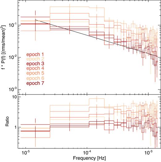
1.5–10.0 keV PSDs with rms normalization for the three sections and 2011 data. The data are Poisson noise subtracted. The bottom panel shows the ratio to the 2011 data.
In Section 4.5 we present a CARMA analysis of the XMM–Newton data spanning ∼30 d. The resulting PSD shows a low-frequency break at ∼10−5 Hz, with slope α < 1 down to low frequencies. The output form the CARMA MCMC runs can be used to assess the stationarity of the light curve. If the source is stationary, the residuals to the model fit should follow a standard normal distribution (Kelly et al. (2014)). The residuals from the 0.3–10.0 keV band CARMA(3,2) model show a discrepancy with a standard normal in Fig. A4. This provides further evidence for a non-stationary X-ray power spectrum in IRAS 13224–3809.
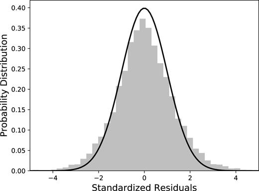
Residuals (grey) from the CARMA(3,2) run for the 0.3–10.0 keV band compared to a standard normal distribution (black).
We search for the presence of any additional components below ∼10−7 Hz using the ∼6 yr Swift light curve (see Buisson et al. 2018). The best-fitting model is shown in Fig. A5 along with the 99 per cent confidence interval. The model is consistent with the 30 d PSD and no additional components are seen down to 5 × 10⁻⁹ Hz.
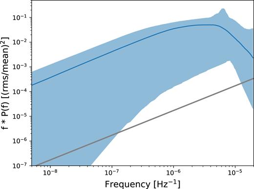
CARMA(3,1) PSD modelling of the ∼6 yr Swift XRT 0.3–10.0 keV light curve. The shaded region is the 99 per cent confidence interval on the model.
