


ABSTRACT
We have investigated the jet-linked X-ray emission from highly radio-loud quasars (HRLQs; log R > 2.5) at high redshift. We studied the X-ray properties of 15 HRLQs at z > 4, using new Chandra observations for six objects and archival XMM–Newton and Swift observations for the other nine. We focused on testing the apparent enhancement of jet-linked X-ray emission from HRLQs at z > 4. Utilizing an enlarged (24 objects) optically flux-limited sample with complete X-ray coverage, we confirmed that HRLQs at z > 4 have enhanced X-ray emission relative to that of HRLQs at z ≈ 1–2 with matched UV/optical and radio luminosity, at a 4.0–4.6 σ level; the X-ray enhancements are confirmed considering both two-point spectral indices and inspection of broad-band spectral energy distributions. The typical factor of enhancement is revised to |$1.9^{+0.5}_{-0.4}$|, which is smaller than but consistent with previous results. A fractional inverse-Compton/cosmic microwave background (IC/CMB) model can still explain our results at high redshift, which puts tighter constraints on the fraction of IC/CMB X-rays at lower redshifts, assuming the physical properties of quasar jets do not have a strong redshift dependence. A dominant IC/CMB model is inconsistent with our data.
1 INTRODUCTION
Quasars (and their parent population of active galactic nuclei, AGNs) are ultimately powered by the accretion process, where gravitational binding energy is released as matter falls into the deep gravitational potential well of the supermassive black hole (SMBH) located in the central region of the host galaxy. The released energy is mainly in the form of quasi-thermal optical/UV photons, likely radiated from an optically thick accretion disc, with a mass-to-radiation conversion efficiency of ∼0.1. Accompanying the accretion process, a pair of highly collimated relativistic jets can sometimes launch from the vicinity of the SMBH, perhaps by tapping the spin energy of the SMBH, and extend to galactic and intergalactic scales (e.g. Begelman, Blandford & Rees 1984). These quasar jets can radiate across the whole electromagnetic spectrum and are most easily detected in the radio band. According to the flux ratio at rest-frame 5 GHz versus 4400 Å, i.e. the radio-loudness parameter R (|$\equiv f_{\rm 5\,\,GHz}/f_{4400\rm~{\mathring{\rm A} }}$|; Kellermann et al. 1989), the quasar population is divided into radio-quiet quasars (RQQs; R < 10) and radio-loud quasars (RLQs; R > 10).1 RLQs are found to be the minority, making up ∼10 per cent of the quasar population (e.g. Ivezić et al. 2004).
X-ray emission is nearly universal from accreting SMBHs (Brandt & Alexander 2015, and references therein). For RQQs, the primary power-law emission in X-rays (∼1–100 keV) is thought to be created by UV photons from the accretion disc inverse-Compton (IC) scattering off electrons in an optically thin and hot (≈109 K) plasma above the disc, the so-called ‘accretion-disc corona’. RLQs have an additional jet-linked X-ray component (e.g. Wilkes & Elvis 1987; Worrall et al. 1987), which can outshine the coronal X-ray emission by a factor of ≈ 3–30 in cases of large radio loudness (e.g. Miller et al. 2011, Miller11 hereafter). This jet-linked X-ray emission is mainly attributed to IC emission of relativistic (non-thermal) electrons that are accelerated by shocks/magnetic reconnection in the jet.
The quasar population has long been known to show strong cosmological evolution in number density (e.g. Schmidt 1968; McGreer et al. 2013; Yang et al. 2016), with RLQs likely evolving differently from RQQs (e.g. Ajello et al. 2009). However, the spectral energy distributions (SEDs) of quasars generally show little evolution to z > 6. In X-rays, RQQs at z > 4 have similar spectral (e.g. Brandt et al. 2002; Vignali et al. 2003; Shemmer et al. 2006; Nanni et al. 2017) and variability (e.g. Shemmer et al. 2017) properties as those of appropriately matched RQQs at lower redshift, in line with quasar properties in other bands (e.g. Jiang et al. 2006; Fan 2012). Moderately radio-loud quasars (1 < log R < 2.5) at z > 4 also have similar X-ray properties to their low-redshift counterparts (e.g. Bassett et al. 2004; Lopez et al. 2006; Saez et al. 2011), while the highly radio-loud quasars (HRLQs; log R > 2.5) show an apparent enhancement in the X-ray band at high redshift (Wu et al. 2013, Wu13 hereafter).
These X-ray studies of high-z RLQs are inconsistent with one of the leading models for quasar jets based on X-ray photometric imaging of low-z objects, where the IC process involving cosmic microwave background (CMB) photons is thought to play an important role. CMB photons have long been proposed to be seeds for the IC process that can effectively produce X-rays (e.g. Felten & Morrison 1966; Harris & Grindlay 1979; Feigelson et al. 1995). One relevant case is quasar lobes (e.g. Brunetti et al. 1999), where relativistic electrons are coupled with CMB photons and produce X-ray emission. After the discovery of the X-ray jet of PKS 0637−752 (Chartas et al. 2000; Schwartz et al. 2000) by Chandra, the application of the IC/CMB mechanism to kpc-scale quasar jets become popular. The X-ray jet of PKS 0637−752 is so luminous (relative to the optical) that it cannot be readily produced by other mechanisms (e.g. Schwartz et al. 2000; Harris & Krawczynski 2002), while a modern version of the IC/CMB model can explain radio-to-X-ray SEDs of individual jet knots and maintains the assumption of equipartition. This modern version of the IC/CMB model has two essential requirements: that the kpc-scale quasar jets are relativistic with bulk Lorentz factor ∼10 and are observed at small angles to our line of sight (Tavecchio et al. 2000; Celotti, Ghisellini & Chiaberge 2001). These two ingredients naturally explain the one-sidedness of many X-ray jets that are commonly detected in surveys of low-z quasar jets (e.g. Sambruna et al. 2004; Kataoka & Stawarz 2005; Marshall et al. 2005)
In spite of the apparent initial success of the (beamed) IC/CMB model in low-z objects, X-ray studies of high-z RLQs provide a critical piece of evidence against using this model to explain the dominant majority of the X-ray emission from quasar jets. The CMB energy density has a strong cosmological evolution (UCMB ∝ (1 + z)4), which is not reproduced in the jet-linked X-rays from RLQs. The X-ray luminosities of the few resolved jets at high redshift are usually only a few per cent that of the cores (similar to large-scale jets at low redshift; e.g. Siemiginowska et al. 2003; Yuan et al. 2003; Saez et al. 2011; Cheung et al. 2012; McKeough et al. 2016), and useful X-ray upper limits on extended jet emission exist for many more RLQs (e.g. Bassett et al. 2004; Lopez et al. 2006; Wu13). Additionally, the jet-linked core emission (which could include X-ray emission from foreshortened kpc-scale jets in some systems) at high redshift does not show the dramatic enhancement predicted by the IC/CMB model (e.g. Bassett et al. 2004; Lopez et al. 2006; Miller11; Wu13). Furthermore, there are other multiple lines of evidence against the most-straightforward IC/CMB model: the tension between the observed and predicted relative brightness distribution in the X-ray and radio bands, the excessive requirement for the jet power, the need for extremely small viewing angles, the high polarization of the optical emission from some jet knots suggestive of synchrotron emission, and the non-detections of γ-ray emission from quasar jets (e.g. Harris & Krawczynski 2006; Uchiyama et al. 2006; Meyer & Georganopoulos 2014). Alternative models for the luminous low-z X-ray jets often involve an ad hoc high-energy synchrotron component (e.g. Atoyan & Dermer 2004).
Even if the IC/CMB process does not play a dominant role, we should expect some IC/CMB X-ray emission from AGN jets; the question is the level of contribution from this process (e.g. Harris & Krawczynski 2006), which could be revealed by studying high-redshift radio-luminous quasars in X-rays. HRLQs rank as the top 5 per cent of the RLQ population in radio loudness (see Fig. 1), and HRLQs at z > 4 harbour the most-powerful relativistic jets from the first SMBHs in the early universe, when the CMB photon field is >625 times more intense than now. Wu13 compared the X-ray emission of a sample of HRLQs at z > 4 (median z = 4.4) with that of another sample of HRLQs at z < 4 (median z = 1.3) with matched UV/optical and radio luminosity, and found an X-ray enhancement for the HRLQs at z > 4 at a 3–4σ level. HRLQs at z > 4 have stronger X-ray emission than their counterparts at z < 4, by a factor of ≈ 3 on average. There is also evidence for a 5σ X-ray enhancement in another independent sample of HRLQs at z =3–4 that is drawn from Miller11.
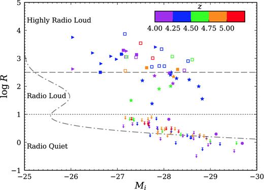
The distribution of z > 4 HRLQs in the log R–Mi plane, compared to moderately radio-loud quasars and RQQs at z > 4. The filled squares and triangles are the Chandra Cycle 17 objects and archival data objects, respectively. The open squares are the HRLQs of Wu13. The filled stars are moderately radio-loud quasars at z > 4 (Bassett et al. 2004; Lopez et al. 2006; Miller11). The filled circles and downward arrows represent the radio-quiet SDSS quasars at z > 4 that have sensitive X-ray coverage. All the symbols are colour-coded based on their redshifts using the colour bar at the top right of the figure. The dotted and dashed lines indicate our criteria for RLQs and HRLQs. The dash-dotted curve (with an arbitrary linear scale) shows the radio-loudness distribution of SDSS quasars (Ivezić et al. 2004), which shows that HRLQs reside in the tail of high radio-loudness.
To explain the redshift dependence of the relative X-ray enhancement of HRLQs, Wu13 proposed a fractional IC/CMB model, in which CMB photons are relevant only on the scale of ∼1–5 kpc, with photons from the central engine dominating at smaller distance (e.g. Ghisellini & Tavecchio 2009). At scales beyond a few kpc, the jet has already decelerated so that CMB photons in the rest frame of the jet are not intense enough for the IC/CMB mechanism to be significant (e.g. Mullin & Hardcastle 2009; Meyer et al. 2016; Marshall et al. 2018). The cosmologically evolving IC/CMB X-ray emission only contributes a fraction of the overall X-ray emission from HRLQs with the rest coming from (redshift-independent) IC processes on small scales that involve seed photons from the central engine. The fraction was estimated to be ≈6 per cent at z ≈ 1.3 by Wu13 and rises with redshift. Alternatively, the results of Wu13 can also be explained by a scenario where the star-forming activity of the hosts provides infrared/optical photons that are IC scattered into the X-ray band. This scenario requires the host galaxies of high-redshift quasars to have enhanced star-formation activity (e.g. Wang et al. 2011; Mor et al. 2012; Netzer et al. 2014). In this case, the IC/CMB process becomes even less relevant.
The sample of 17 HRLQs at z > 4 used in Wu13 suffers from heterogeneity and limited size, which renders their ≈4σ results only suggestive. Here, we aim at confirming the X-ray enhancement of HRLQs using a larger and more uniformly selected sample. We obtained new Chandra observations for six HRLQs at z > 4 and present their X-ray properties in the paper. We also present X-ray properties of another nine HRLQs at z > 4 that have archival Swift or XMM–Newton data. We describe our sample selection in Section 2, and X-ray data analyses in Section 3. In the following sections, we adopt a flat ΛCDM cosmology, with H0 = 70.0 km s−1 Mpc−1 and Ωm = 0.3 (e.g. Planck Collaboration XIII 2016).
2 SAMPLE SELECTION
We started with a primary sample that was selected by Wu13 from the Sloan Digital Sky Survey (SDSS) quasar catalogue Data Release 7 (DR7; covering 9380 deg2 of sky area; Schneider et al. 2010) and NED.2 They have utilized the 1.4 GHz NRAO VLA Sky Survey (NVSS; Condon et al. 1998), which has provided homogeneous radio coverage for the full sky area of ≈ 34 000 |$\deg ^2$| north of δ = −40°. For high-z RLQs identified in current wide-field optical/UV surveys (i.e. mi ≲ 21), if an object satisfies the HRLQ criterion of log R > 2.5, it should have been detected by the NVSS given its sensitivity (≈ 2.5 mJy).3 Among the resulting sample of 26 HRLQs,4 17 with sensitive X-ray coverage (typically reaching FX ≈ 10−14 er g cm−2 s−1 or better in the observed-frame 0.5–2 keV band) have been studied in Wu13 while another two were studied by Sbarrato et al. (2015). The other five objects (see table 2 of Wu13) with mi < 21 and lacking sensitive X-ray coverage were awarded Chandra time in Cycle 17. The remaining two objects are fainter than mi = 21. See Table 1 for the Chandra Cycle 17 observation log.5
X-ray observation log.
| Object name | RA | Dec. | Instr. | za | Obs. date | Obs. IDb | Exp. timec | FLd | Ref.e |
|---|---|---|---|---|---|---|---|---|---|
| (deg) | (deg) | (ks) | |||||||
| Chandra Cycle 17 objects | |||||||||
| SDSS J003126.79+150739.5 | 7.8617 | 15.1277 | ACIS-S | 4.296 | 2016/06/09 | 18442 | 5.4 | N | – |
| B3 0254+434 | 44.4962 | 43.6438 | ACIS-S | 4.067 | 2015/12/12 | 18449 | 5.5 | Y | 1 |
| SDSS J030437.21+004653.5 | 46.1551 | 0.7816 | ACIS-S | 4.266 | 2015/11/28 | 18443 | 5.9 | Y | – |
| SDSS J081333.32+350810.8 | 123.3889 | 35.1363 | ACIS-S | 4.929 | 2015/12/19 | 18444 | 6.0 | Y | – |
| SDSS J123142.17+381658.9 | 187.9257 | 38.2830 | ACIS-S | 4.115 | 2016/02/13 | 18445 | 6.0 | N | – |
| SDSS J123726.26+651724.4 | 189.3594 | 65.2901 | ACIS-S | 4.301 | 2016/08/21 | 18446 | 7.9 | N | – |
| SDSS J124230.58+542257.3 | 190.6274 | 54.3826 | ACIS-S | 4.750 | 2016/05/16 | 18447 | 4.9 | Y | – |
| PMN J2314+0201 | 348.7030 | 2.0309 | ACIS-S | 4.110 | 2016/01/15 | 18448 | 5.9 | Y | 2 |
| Archival data objects | |||||||||
| SDSS J083549.42+182520.0 | 128.9559 | 18.4222 | XRT | 4.412 | 2017/01/10–2017/05/25 | 00087221001 | 45.8 | N | – |
| SDSS J102107.57+220921.4 | 155.2816 | 22.1560 | EPIC-pn | 4.262 | 2008/05/30 | 0406540401 | 8.1 | N | – |
| SDSS J111323.35+464524.3 | 168.3473 | 46.7568 | XRT | 4.468 | 2016/07/05–2016/07/20 | 00703176000 | 52.9 | N | – |
| SDSS J134811.25+193523.6 | 207.0469 | 19.5899 | XRT | 4.404 | 2017/11/29–2018/01/15 | 00087542001 | 46.6 | Y | – |
| SDSS J153533.88+025423.3 | 233.8912 | 2.9065 | XRT | 4.388 | 2017/01/06–2017/01/26 | 00087222001 | 26.4 | Y | – |
| SDSS J160528.21+272854.4 | 241.3675 | 27.4818 | EPIC-pn | 4.024 | 2011/05/01 | 0655571401 | 11.0 | N | – |
| SDSS J161216.75+470253.6 | 243.0698 | 47.0482 | XRT | 4.350 | 2017/11/08–2017/12/13 | 00088204001 | 48.7 | N | – |
| PMN J2134−0419 | 323.5501 | −4.3194 | XRT | 4.346 | 2013/06/16–2013/06/20 | 00032624001 | 25.1 | Y | 2 |
| SDSS J222032.50+002537.5 | 335.1354 | 0.4271 | XRT | 4.220 | 2013/07/01–2013/08/29 | 00032626001 | 43.5 | Y | - |
Notes.aRedshifts for objects in the SDSS DR7 quasar catalogue and the SDSS DR14 quasar catalogue are from Hewett & Wild (2010) and Pâris et al. (2018), respectively. Redshifts for other objects are from NED.
bWe merged multiple observations of the same target for archival Swift/XRT data, while only the first observation is listed in the table. The full observation IDs are 00087221001–00087221023 for SDSS J083549.42+182520.0, 00703176000–00703176011 for SDSS J111323.35+464524.3, 00087542001–00087542016 for SDSS J134811.25+193523.6, 00087222001–00087222007 for SDSS J153533.88+025423.3, 00032624001–00032624003 for PMN J2134−0419, 00087543001–00087543018 (excluding 00087543013 because it lacks PC-mode exposures) for SDSS J161216.75+470253.6, and 00032626001–00032626005 for SDSS J222032.50+002537.5.
cFor archival XRT data, this column refers to the LIVETIME from the merged event lists. For archival EPIC data, this column refers to the LIVETIME of the EPIC-pn CCD on which the source is detected, after filtering background flares.
dThis column indicates whether the quasar is included in the flux-limited (FL) sample or not.
We furthermore searched in the SDSS quasar catalogue Data Release 14 (DR14; Pâris et al. 2018) for HRLQs at z = 4.0–5.5, and found another 16 HRLQs that were matched to the Faint Images of the Radio Sky at Twenty-centimeters survey (FIRST; Becker, White & Helfand 1995), which is designed to coincide with the primary region of sky covered by the SDSS. Since the FIRST survey has a detection limit of ≈1 mJy, all additional HRLQs in the SDSS quasar catalogue DR14 with mi < 21 can be detected by FIRST if they satisfy the criterion of log R > 2.5.6 Another high-z HRLQ, B3 0254+434 (Amirkhanyan & Mikhailov 2006), was selected in NED using the same method as Wu13. See Section 3.5 for details on the calculations of optical and radio luminosities and radio-loudness parameters using optical and radio fluxes. We retrieved the available sensitive archival X-ray observations from HEASARC7 of these new objects. Five high-z HRLQs (SDSS J083549.42+182520.0, SDSS J111323.35+464524.3, SDSS J134811.25+193523.6, SDSS J153533.88+025423.3, and SDSS J161216.75+470253.6) have useful deep (≳25 ks) Swift X-ray observations. Two more (SDSS J102107.57+220921.4 and SDSS J160528.21+272854.4) are matched with the XMM–Newton serendipitous-source catalogue 3XMM-DR8 (Rosen et al. 2016). See Table 1 for the observation log of the relevant Swift and XMM–Newton archival data.8 B3 0254+434 was awarded Chandra time in Cycle 17. The rest of the objects that lack publicly released sensitive archival X-ray observations are listed in Table 2.
HRLQs at z > 4 without vailable sensitive archival X-ray data.
| Object name | RA (J2000) | Dec. (J2000) | z | mi | Mi | |$f_{1.4\,\,\rm GHz}$| | log R |
|---|---|---|---|---|---|---|---|
| (deg) | (deg) | (mJy) | |||||
| SDSS J082511.60+123417.2 | 126.2984 | 12.5715 | 4.378 | 20.71 | −26.46 | 16.7 | 2.66 |
| SDSS J094004.80+052630.9a | 145.0200 | 5.4419 | 4.503 | 20.80 | −26.44 | 55.7 | 3.22 |
| SDSS J104742.57+094744.9 | 161.9274 | 9.7958 | 4.252 | 20.29 | −26.77 | 18.9 | 2.58 |
| SDSS J115605.44+444356.5 | 179.0227 | 44.7324 | 4.310 | 21.06 | −26.08 | 66.2 | 3.41 |
| SDSS J125300.15+524803.3 | 193.2506 | 52.8009 | 4.115 | 21.33 | −25.66 | 55.9 | 3.47 |
| SDSS J140025.40+314910.6a | 210.1059 | 31.8196 | 4.640 | 20.28 | −26.89 | 20.2 | 2.61 |
| SDSS J153830.71+424405.6 | 234.6280 | 42.7349 | 4.099 | 20.77 | −26.18 | 11.7 | 2.58 |
| SDSS J154824.01+333500.1a | 237.1001 | 33.5834 | 4.678 | 20.35 | −26.80 | 37.6 | 2.93 |
| SDSS J165539.74+283406.7 | 253.9156 | 28.5685 | 4.048 | 20.42 | −26.51 | 23.0 | 2.73 |
Note.aChandra/ACIS observations have been conducted or scheduled for SDSS J094004.80+052630.9, SDSS J140025.40+314910.6, and SDSS J154824.01+333500.1. Their X-ray data will become public after their proprietary periods.
We plotted the apparent i-band magnitudes and the X-ray coverage of all the HRLQs that were selected in this paper and in Wu13 in Fig. 2, where the objects with sensitive X-ray coverage were plotted as blue dots, while objects without sensitive X-ray coverage were plotted as blue circles. We here define our flux-limited high-z sample by applying an optical flux limit of mi ≤ 20.26. The 24 HRLQs that satisfy this flux cut all have sensitive X-ray coverage, among which 21 were selected in Wu13 and three (B3 0254+434, SDSS J134811.25+193523.6, and SDSS J153533.88+025423.3) were selected in this paper. In comparison with Wu13, our flux-limited sample is not only larger (twice as large) but also complete in its X-ray coverage (24/24 versus 12/15), thus suffering less from selection biases. For comparison, the optical flux limit of the Wu13 flux-limited sample was mi = 20.
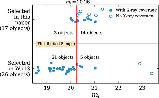
The mi of the 43 HRLQs that were selected in this paper (17 objects) and in Wu13 (26 objects). The blue solid circle are the objects with sensitive X-ray coverage, while blue open circles are the objects without sensitive X-ray coverage. The vertical red line marks the magnitude cut for the flux-limited sample. Object locations along the vertical axis are only used to distinguish between the objects selected by Wu13 and in this paper. Additionally, each data point is also randomly perturbed in the vertical direction to avoid overlapping.
We have plotted the rest-frame UV spectra for the members of our sample of HRLQs that are in the SDSS quasar catalogues in Fig. 3. It is apparent from their spectra that all of them are broad-line quasars, instead of BL Lac objects; the observed emission from the accretion disc and broademission-lineregion in the optical/UV is free from strong contamination by boosted jet emission. The rest-frame UV spectra of the objects that were not in the SDSS quasar catalogues can be found in Hook et al. (2002) for PMN J2134−0419 and PMN J2314+0201 and Amirkhanyan & Mikhailov (2006) for B3 0254+434. The spectra of these three objects show features of broad-line quasars as well. We also plotted the radio and optical/UV luminosities of high-z HRLQs against general RLQs in Fig. 4; their monochromatic luminosities are among the highest in both the radio and optical/UV bands, with our sample extending to a slightly fainter range than Wu13 in the optical/UV.
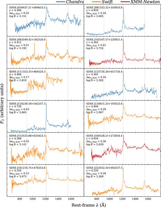
The rest-frame UV spectra of the HRLQs that are in the SDSS quasar catalogues, ordered by RA. The object name, redshift (z), Δαox,RQQ (the difference between the measured value of αox and the expected αox,RQQ, see the description of Column 16 in Section 3.5), and radio-loudness parameter (log R) are shown in the top-left corner in each panel. The spectra do not show strong dependence on Δαox,RQQ, z, or log R. We have plotted the spectra with different colours according to their X-ray data as labelled, where the Chandra Cycle 17 objects are blue. The y-axis is in linear scale with arbitrary units. Each spectrum has been smoothed using a 21-pixel boxcar filter. Two emission lines (Ly α λ1216 and C iv λ1549) and the Lyman limit have been labelled with the dotted vertical lines. Similar spectra can be found in fig. 3 of Wu13 for the Wu13 objects.
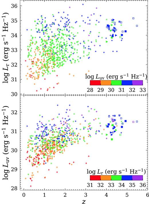
The radio (rest-frame 5 GHz; upper panel) and UV (rest-frame 2500 Å; lower panel) luminosities, plotted against redshift. The filled squares and triangles are the Chandra Cycle 17 objects and archival-data objects, respectively. The open squares are the high-redshift HRLQs of Wu13. The plus signs are the radio-loud and radio-intermediate objects in the full sample of Miller11. The upper and lower panels are colour-coded based on UV and radio luminosity, respectively. Due to selection on R and mi, our sample and the sample of Wu13 are composed of among the most-luminous objects in both the radio and UV bands.
RLQs with extended radio morphologies have systematically larger radio-loudness parameters and also more powerful radio cores than quasars with compact radio morphologies (e.g. Lu et al. 2007). Our selection of HRLQs based on high R thus should not cause a bias toward including quasars with core-only morphologies or low intrinsic jet/core radio flux ratios, unless the cores dominate the radio fluxes for quasars with extended morphologies or RLQs jets evolve with redshift. High-redshift RLQs usually show compact radio morphology with few having apparently extended structures, which is probably due to the steeper radio slope (αr < −0.5) and the cosmological surface brightness dimming of diffuse radio emission, i.e. (1 + z)−4. Fifteen out of the 17 objects (except for B3 0254+434 and SDSS J1237+6517) in Table 1 are within the footprint of the FIRST survey, and 13 of them only show unresolved radio cores (<5 arcsec, or <35 kpc). The remaining two (SDSS J0813+3508 and SDSS J2220+0025) are resolved into multiple components (Becker et al. 1995; Hodge et al. 2011) and have a linear extent of ≈10 arcsec (≈70 kpc). The radio flux of the extended component of SDSS J0813+3508 is about half that of the core, while the extended radio component is brighter than the core for SDSS J2220+0025. Several quasars in Table 1 have been observed using very long baseline interferometry (VLBI). Specifically, SDSS J0813+3508 and SDSS J1242 + 5422 were observed by Frey et al. (2010) at 1.6 GHz and 5 GHz, and PMN J2134−0419 and SDSS J2220+0025 were observed by Cao et al. (2017) at 1.7 GHz and 5 GHz. These observations can resolve structures on the scale of 1.2–25 mas (≈8–160 pc). At such small scales, these quasars are often mildly resolved and show a compact core with a one-sided jet (SDSS J0813+3508 and PMN J2134−0419) or an unresolved core (SDSS J1242+5422 and SDSS J2220+0025). Note that VLBI observation of PMN J2314−0419 shows evidence of strong Doppler boosting (Cao et al. 2017).
3 X-RAY DATA ANALYSES AND MULTIWAVELENGTH PROPERTIES
In the below, we define the soft band, hard band, and full band to be 0.5–2, 2.0–8.0, and 0.5–8 keV in the observed frame, respectively.
3.1 Chandra data analyses
Eight RLQs were targeted with the Advanced CCD Imaging Spectrometer (ACIS; Garmire et al. 2003) onboard Chandra, using the back-illuminated S3 chip. The Chandra data (see Table 1) were first reprocessed using the standard ciao (v4.9) routine chandra_repro and the latest caldb (v4.7.3). X-ray images and exposure maps were then generated using fluximage in the three observed bands, where the effective energy that was used to calculate the exposure map was chosen to be the geometric mean of the limits of each band. All of the sources were detected by wavdetect (Freeman et al. 2002) in at least two bands with a detection threshold 10−6 and wavelet scales of 1, |$\sqrt{2}$|, 2, |$2\sqrt{2}$|, and 4 pixels. We performed statistical tests on the X-ray images and found no extended structure or large-scale jets. Furthermore, we constrained any extended X-ray jets to be ≳3–25 times fainter than the cores. (see details in Appendix A). Raw source and background counts were extracted using dmextract. The source region was a circle with a radius of 2.0 arcsec, centred at the X-ray position from wavdetect, and the background region was a concentric annulus with an inner radius of 5.0 arcsec and an outer radius of 20.0 arcsec. The offset between the X-ray position and optical position of each source ranges from 0.2 to 0.7 arcsec. All the background regions are free of X-ray sources except for that of SDSS J123142.17+381658.9, in which we have excluded a source detected by wavdetect. The circular source region encloses |${\approx }95.9{{\ \rm per\ cent}}$| of the total energy at 1 keV and |${\approx }90.6{{\ \rm per\ cent}}$| of the total energy at 4 keV.9 We also extracted source and background spectra using specextract,10 which simultaneously produces response matrix files (RMFs) and ancillary response files (ARFs).11
3.2 Swift data analyses
Data reduction of the Swift/X-ray Telescope (XRT; Burrows et al. 2005) observations was performed using standard routines in ftools integrated in heasoft (v6.21).12 Each HRLQ has multiple observations (see Table 1). For each observation, the cleaned event list and exposure map were created using xrtpipeline and xrtexpomap, respectively. We only used XRT data in photon-counting (PC) mode. The event lists and exposure maps of different observations were then merged using xselect and ximage, respectively. We extracted photons in the three bands from circular regions centred at the source positions with radii of ∼60 arcsec except for SDSS J111323.35+464524.3 and SDSS J161216.75+470253.6, for which we have adopted a radius of 25 arcsec to avoid contamination by nearby sources. These source-extraction regions enclose ∼80–90 per cent (73 per cent for SDSS J111323.35+464524.3 and 80 per cent for SDSS J161216.75+470253.6) of the total energy at 1 keV. Photons from circular source-free regions of radii that are more than twice as large as the source region were extracted to estimate the background level. We also extracted source and background spectra using xselect, and created ARFs using xrtmkarf, which simultaneously provides the corresponding RMFs.
3.3 XMM–Newton data analyses
SDSS J102107.57+220921.4 and SDSS J160528.21+272854.4 were serendipitously observed by XMM–Newton (see Table 1).13 Data reduction was performed using sas (v16.1.0) and the latest Current Calibration Files (as of March 2018). We only utilized the data from the pn CCDs of the European Photon Imaging Camera (EPIC-pn; Strüder et al. 2001) onboard XMM–Newton. The data were reprocessed and cleaned using epproc, and high-background flaring periods were filtered using espfilt. We created images and exposure maps using evselect and eexpmap and then performed source detection using eboxdetect.14 Both targets were detected in the full and soft bands, and the offsets between the X-ray positions and optical positions are ∼1–2 arcsec (Rosen et al. 2016). We extracted photons from source regions that are defined by a circle with a radius of 40 arcsec, centred at the optical position. Background photons were extracted from source-free circular regions on the same chips, with radii of 60 and 50 arcsec for SDSS J102107.57+220921.4 and SDSS J160528.21+272854.4, respectively. The encircled-energy fraction is ≈86 per cent for both sources at 1 keV, which is calculated using the point spread function (PSF) images created by psfgen. We also extracted spectra using evselect and created corresponding RMFs and ARFs using rmfgen and arfgen, respectively.
3.4 Source detection and photometry
In the below, analyses of Chandra/ACIS, Swift/XRT, and XMM–Newton/EPIC data were conducted in a unified way. Using the raw source and background event counts, we calculated the binomial no-source probability (referred to as PB in this paper; Weisskopf et al. 2007)15 to test the significance of the source signal in each band, and took cases with PB ≤ 0.01 as detections. We calculated net counts from the HRLQs (with aperture corrections) and their 1σ intervals using aprates16 within ciao. For each band without a detection (PB > 0.01), we gave a 90 per cent confidence upper limit (Kraft, Burrows & Nousek 1991).
We then proceeded by calculating the hardness ratio of each source. The 68 per cent bounds of hardness ratio were calculated using the Bayesian approach of Park et al. (2006). Using the response files and modelflux (another ciao routine),17 we calculated the expected HRs of Galactic-absorbed power-law spectra with a range of photon indices, from which we calculated the effective power-law photon index (ΓX) of each source. The results of the photometry are listed in Table 3. SDSS J124230.58+542257.3 has a noticeably large effective photon index, and deeper X-ray observations in the future might help to improve our understanding of it.18
X-ray net counts, hardness ratio, and effective photon index.
| Object name | Net X-ray counts | Band ratioa | ΓX | ||
|---|---|---|---|---|---|
| Full band | Soft band | Hard band | |||
| (0.5–8 keV) | (0.5–2 keV) | (2–8 keV) | |||
| Chandra Cycle 17 objects | |||||
| SDSS J003126.79+150739.5 | |$14.8^{+4.4}_{-3.6}$| | |$12.5^{+4.0}_{-3.3}$| | |$2.1^{+2.0}_{-1.3}$| | |$0.17^{+0.09}_{-0.14}$| | |$2.43^{+1.20}_{-0.33}$| |
| B3 0254+434 | |$110.6_{-10.5}^{+11.2}$| | |$60.4_{-7.6}^{+8.3}$| | |$50.7_{-7.1}^{+7.8}$| | |$0.84_{-0.20}^{+0.13}$| | |$1.44_{-0.11}^{+0.21}$| |
| SDSS J030437.21+004653.5 | |$10.5^{+3.8}_{-3.0}$| | |$9.4^{+3.5}_{-2.8}$| | <4.1 | <0.44 | >1.79 |
| SDSS J081333.32+350810.8 | |$28.7_{-5.2}^{+5.9}$| | |$16.6_{-3.8}^{+4.6}$| | |$12.1_{-3.3}^{+4.0}$| | |$0.73_{-0.32}^{+0.19}$| | |$1.35_{-0.17}^{+0.44}$| |
| SDSS J123142.17+381658.9 | |$25.3^{+5.5}_{-4.9}$| | |$15.6^{+4.4}_{-3.7}$| | |$9.8^{+3.7}_{-3.0}$| | |$0.63^{+0.21}_{-0.29}$| | |$1.37^{+0.44}_{-0.21}$| |
| SDSS J123726.26+651724.4 | |$13.6^{+4.2}_{-3.5}$| | |$10.4^{+3.7}_{-3.0}$| | |$3.1^{+2.4}_{-1.6}$| | |$0.30^{+0.16}_{-0.21}$| | |$1.92^{+0.90}_{-0.30}$| |
| SDSS J124230.58+542257.3 | |$15.8^{+4.5}_{-3.8}$| | |$13.5^{+4.1}_{-3.5}$| | |$2.1^{+2.0}_{-1.3}$| | |$0.16^{+0.09}_{-0.12}$| | |$2.38^{+1.13}_{-0.33}$| |
| PMN J2314+0201 | |$43.5^{+7.2}_{-6.5}$| | |$25.0^{+5.5}_{-4.8}$| | |$18.6^{+4.9}_{-4.2}$| | |$0.74^{+0.20}_{-0.25}$| | |$1.33^{+0.30}_{-0.17}$| |
| Archival data objects | |||||
| SDSS J083549.42+182520.0 | 205.2|$^{+17.1}_{-16.9}$| | 135.3|$^{+13.9}_{-13.3}$| | 69.8|$^{+10.5}_{-10.1}$| | 0.52|$^{+0.08}_{-0.09}$| | 1.56|$^{+0.15}_{-0.10}$| |
| SDSS J102107.57+220921.4 | 49.8|$^{+13.9}_{-14.2}$| | 37.7|$^{+9.6}_{-9.4}$| | <26.6 | <0.71 | >1.30 |
| SDSS J111323.35+464524.3 | |$33.3_{-7.5}^{+8.2}$| | |$21.9_{-5.9}^{+6.6}$| | |$11.4_{-4.4}^{+5.1}$| | |$0.52_{-0.29}^{+0.17}$| | |$1.51_{-0.21}^{+0.59}$| |
| SDSS J134811.25+193523.6 | 78.4|$^{+12.7}_{-12.0}$| | 52.5|$^{+10.5}_{-9.8}$| | 26.0|$^{+7.4}_{-6.8}$| | 0.49|$^{+0.14}_{-0.17}$| | 1.56|$^{+0.32}_{-0.18}$| |
| SDSS J153533.88+025423.3 | 324.3|$^{+21.7}_{-21.5}$| | 185.7|$^{+16.9}_{-16.3}$| | 138.6|$^{+14.2}_{-13.7}$| | 0.75|$^{+0.08}_{-0.10}$| | 1.32|$^{+0.11}_{-0.08}$| |
| SDSS J160528.21+272854.4 | <61.5 | 26.8|$^{+10.9}_{-10.8}$| | <28.4 | - | - |
| SDSS J161216.75+470253.6 | |$23.1_{-6.0}^{+6.6}$| | |$19.1_{-5.0}^{+5.7}$| | <10.1 | <0.53 | >1.50 |
| PMN J2134−0419 | |$70.7_{-10.7}^{+11.2}$| | |$49.3_{-8.5}^{+9.1}$| | |$21.4_{-6.2}^{+7.0}$| | |$0.43_{-0.18}^{+0.12}$| | |$1.70_{-0.18}^{+0.38}$| |
| SDSS J222032.50+002537.5 | |$44.8_{-9.2}^{+9.7}$| | |$37.6_{-7.6}^{+8.2}$| | <15.8 | <0.42 | >1.76 |
Note.aThe band ratio here refers to the number of hard-band counts divided by the number of the soft-band counts.
3.5 X-ray, optical/UV, and radio properties
In Table 4, we summarize the X-ray, optical/UV, and radio properties of our sample of HRLQs, utilizing the results of our X-ray data analyses as well as SDSS and FIRST/NVSS surveys. We explain the content of each column below:
X-ray, optical/UV, and radio properties.
| Object name | mi | Mi | |$N_{\rm H}^{a}$| | C.R.b | |$F_{\rm X}^{ c}$| | |$f_{\rm 2 keV}^{ d}$| | |$\log L_{\rm X}^{e}$| | |$\Gamma _{\rm X}^{f}$| | |$f_{2500\rm~{\mathring{\rm A} }}^{g}$| | |$\log L_{2500\rm~{\mathring{\rm A} }}^{ h}$| | |$\alpha _{\rm r}^{i}$| | |$\log L_{\rm r}^{j}$| | log R | αox | |$\Delta \alpha _{\rm ox, RQQ}^{k}$| | |$\Delta \alpha _{\rm ox, RLQ}^{l}$| |
|---|---|---|---|---|---|---|---|---|---|---|---|---|---|---|---|---|
| (1) | (2) | (3) | (4) | (5) | (6) | (7) | (8) | (9) | (10) | (11) | (12) | (13) | (14) | (15) | (16) | (17) |
| Chandra Cycle 17 objects | ||||||||||||||||
| SDSS J003126.79+150739.5 | 19.99 | −27.16 | 4.43 | |$2.33^{+0.74}_{-0.61}$| | 1.81 | 21.17 | 45.61 | |$2.43^{+1.20}_{-0.33}$| | 0.92 | 31.50 | 0.61 | 34.07 | 2.44 | −1.40 | 0.31 | 0.10 |
| B3 0254+434 | 20.01 | −27.24 | 13.45 | |$10.96^{+1.50}_{-1.38}$| | 7.98 | 34.94 | 46.14 | |$1.44^{+0.21}_{-0.11}$| | 0.56 | 31.25 | 0.06 | 34.66 | 3.29 | −1.23 | 0.44 | 0.15 |
| SDSS J030437.21+004653.5 | 20.15 | −27.09 | 7.26 | |$1.60^{+0.60}_{-0.48}$| | 1.10 | 7.03 | 45.35 | >1.79 | 0.11 | 30.57 | – | 33.85 | 3.15 | −1.23 | 0.35 | 0.11 |
| SDSS J081333.32+350810.8 | 19.15 | −28.30 | 4.91 | |$2.78^{+0.76}_{-0.64}$| | 1.72 | 7.27 | 45.63 | |$1.35^{+0.44}_{-0.17}$| | 0.81 | 31.54 | −0.60 | 34.26 | 2.61 | −1.55 | 0.16 | −0.07 |
| SDSS J123142.17+381658.9 | 20.12 | −26.88 | 1.27 | |$2.58^{+0.73}_{-0.61}$| | 1.52 | 6.22 | 45.43 | |$1.37^{+0.45}_{-0.19}$| | 1.13 | 31.56 | – | 33.82 | 2.14 | −1.63 | 0.08 | −0.10 |
| SDSS J123726.26+651724.4 | 20.46 | −26.63 | 2.03 | |$1.32^{+0.47}_{-0.38}$| | 0.90 | 6.59 | 45.28 | |$1.92^{+0.90}_{-0.30}$| | 0.61 | 31.32 | – | 33.94 | 2.50 | −1.52 | 0.16 | −0.05 |
| SDSS J124230.58+542257.3 | 19.65 | −27.63 | 1.55 | |$2.77^{+0.84}_{-0.71}$| | 1.73 | 21.96 | 45.71 | |$2.38^{+1.13}_{-0.33}$| | 0.42 | 31.23 | −0.56 | 34.01 | 2.67 | −1.24 | 0.43 | 0.21 |
| PMN J2314+0201 | 19.54 | −27.41 | 4.82 | |$4.25^{+0.93}_{-0.81}$| | 2.64 | 10.36 | 45.67 | |$1.33^{+0.33}_{-0.15}$| | 0.72 | 31.36 | −0.27 | 34.62 | 3.13 | −1.47 | 0.21 | −0.06 |
| Archival Data Objects | ||||||||||||||||
| SDSS J083549.42+182520.0 | 20.74 | −26.47 | 3.21 | |$2.95_{-0.30}^{+0.29}$| | 6.17 | 31.74 | 46.11 | |$1.56^{+0.15}_{-0.11}$| | 0.27 | 30.99 | −0.20 | 34.30 | 3.19 | −1.12 | 0.51 | 0.25 |
| SDSS J102107.57+220921.4 | 21.03 | −26.04 | 2.03 | |$4.65_{-1.16}^{+1.19}$| | 2.72 | 14.32 | 45.73 | >1.30 | 0.19 | 30.81 | −0.17 | 34.69 | 3.75 | −1.20 | 0.41 | 0.10 |
| SDSS J111323.35+464524.3 | 20.58 | −26.65 | 1.31 | |$0.63_{-0.12}^{+0.12}$| | 0.95 | 4.64 | 45.30 | |$1.51^{+0.59}_{-0.21}$| | 0.31 | 31.06 | −0.17 | 33.99 | 2.81 | −1.47 | 0.17 | −0.05 |
| SDSS J134811.25+193523.6 | 20.21 | −26.98 | 1.93 | |$1.13_{-0.21}^{+0.23}$| | 2.29 | 11.75 | 45.68 | |$1.56^{+0.34}_{-0.17}$| | 0.44 | 31.19 | −0.20 | 34.28 | 2.97 | −1.37 | 0.29 | 0.04 |
| SDSS J153533.88+025423.3 | 20.08 | −27.10 | 4.44 | |$7.03_{-0.62}^{+0.64}$| | 15.13 | 59.82 | 46.48 | |$1.32^{+0.10}_{-0.09}$| | 0.49 | 31.24 | −0.31 | 34.50 | 3.14 | −1.12 | 0.55 | 0.28 |
| SDSS J160528.21+272854.4 | 20.85 | −26.04 | 3.94 | |$2.44_{-0.98}^{+0.99}$| | 1.59 | 8.12 | 45.44 | – | 0.21 | 30.82 | – | 33.56 | 2.62 | −1.31 | 0.30 | 0.10 |
| SDSS J161216.75+470253.6 | 20.29 | −26.86 | 1.33 | |$0.39_{-0.10}^{+0.12}$| | 0.79 | 4.19 | 45.21 | >1.50 | 0.40 | 31.14 | −0.44 | 34.34 | 3.07 | −1.53 | 0.13 | −0.13 |
| PMN J2134−0419 | 19.30 | −27.84 | 3.55 | |$1.96_{-0.34}^{+0.36}$| | 4.19 | 24.66 | 45.94 | |$1.70^{+0.38}_{-0.18}$| | 0.96 | 31.53 | −0.23 | 35.05 | 3.40 | −1.38 | 0.33 | 0.02 |
| SDSS J222032.50+002537.5 | 19.95 | −27.20 | 4.73 | |$0.86_{-0.17}^{+0.19}$| | 1.85 | 11.36 | 45.56 | >1.76 | 0.26 | 30.93 | – | 34.32 | 3.26 | −1.29 | 0.34 | 0.07 |
Notes.aGalactic neutral hydrogen column density in units of 1020 cm−2.
bCount rate of the in the observed-frame 0.5–2 keV band, in units of 10−3 s−1.
cGalactic absorption-corrected flux in the observed-frame 0.5–2 keV band, in units of 10−14 er g cm−2 s−1.
dFlux density at 2/(1 + z) keV (extrapolated from the observed 0.5–8 keV X-ray emission), in units of 10−32 er g cm−2 s−1 Hz−1.
eThe logarithm of the X-ray luminosity in the rest-frame 2–10 keV band, in units of erg s−1.
fEffective X-ray power-law photon index.
gFlux density observed at 2500(1 + z) Å in units of 10−27 er g cm−2 s−1 Hz−1.
hLogarithm of the monochromatic UV luminosity at rest frame 2500 Å in units of erg s−1 Hz−1.
iRadio spectral index calculated from observed 1.4 GHz and 5 GHz flux, defined as |$f_\nu \propto \nu ^{\alpha _r}$|. If a 5 GHz observation is absent, we take αr = 0 in the following calculation. The radio spectral index of SDSS J0813 + 3508 is from Frey et al. (2010).
jLogarithm of the monochromatic radio luminosity at rest-frame 5 GHz in units of erg s−1 Hz−1.
kThe difference between the measured αox and the expected αox for RQQs with similar UV luminosity, defined by equation (3) of Just et al. (2007).
lThe difference between the measured αox and the expected αox for RLQs with similar UV and radio luminosities, defined by the |$L_{2 \rm keV}$|-L2500Å-|$L_{5\rm GHz}$| relation in table 7 of Miller et al. (2011).
Column (1): the name of the quasar.
Column (2): the apparent i-band magnitude of the quasar.
Column (3): the absolute i-band magnitude of the quasar. The values are preferentially taken from SDSS quasar catalogues (Schneider et al. 2010; Pâris et al. 2018). For objects that are not in the quasar catalogues, we calculated Mi from mi by correcting for the Galactic extinction (Schlafly & Finkbeiner 2011) and using the K-correction in section 5 of Richards et al. (2006).
Column (4): the Galactic neutral hydrogen column density (Dickey & Lockman 1990; Stark et al. 1992).19
Column (5): the count rate in the observed-frame soft X-ray band for the Chandra Cycle 17 objects.
Column (6): the observed X-ray flux in the soft band calculated using modelflux, the effective power-law photon index (see Column 9), and the instrumental response files. The values have been corrected for Galactic absorption.
Column (7): following Wu13, in this column we estimated the observed X-ray flux density at 2/(1 + z) keV (i.e. rest-frame 2 keV), corrected for Galactic absorption. Note that, for objects at z > 4, the rest-frame 2 keV X-rays are below the lower limit of our observed X-ray bands. Thus, we have extrapolated their X-ray spectra using the effective power-law photon index (see Column 9) to lower energies. Note that this is a relatively short extrapolation, generally a factor of ≲ 1.5 times below the lowest energy of our observed X-rays.
Column (8): the logarithm of the rest-frame 2–10 keV luminosity.
Column (9): the effective power-law photon index in the X-ray band. For the sources with only a lower limit or without estimation of ΓX, we have adopted a typical value for RLQs (ΓX = 1.6; e.g. Page et al. 2005), and for SDSS J030437.21+004653.5 and SDSS J161216+470253.6 we have used their lower limits (ΓX = 1.79 and 1.76) in the following analysis. Within a reasonable range (ΓX = 1.4–1.9; e.g. Page et al. 2005), the value of ΓX does not materially affect the results we presented below.
Column (10): the observed flux density at 2500(1 + z) Å (i.e. rest-frame 2500 Å). For objects in the SDSS DR7 quasar catalogue, the values were taken from Shen et al. (2011). For other objects, the values were calculated from their i-band magnitude (Column 3).
Column (12): the radio spectral index αr (|$f_\nu \propto \nu ^{\alpha _{\rm r}}$|) between observed-frame 1.4 and 5 GHz. We obtain 1.4 GHz flux densities from the FIRST or NVSS surveys. The 5 GHz flux densities were mostly from the Green Bank 6-cm survey (Gregory et al. 1996). We obtain the 5 GHz flux density of PMN J2134−0419 from the Parkes-MIT-NRAO survey (Wright et al. 1994). We took the 5 GHz flux density of SDSS J124230.58+542257.3 from its VLBI observation (Frey et al. 2010). The radio counterpart of SDSS J081333.32+350810.8 has a close companion (∼6 arcsec) in the FIRST catalogue, which cannot be identified in the optical and is likely to be associated with SDSS J081333.32+350810.8 as a jet or lobe. We thus took the 1.4 GHz flux density of SDSS J081333.32+350810.8 as the sum of the two radio sources from the FIRST catalogue. Since the radio companion is completely resolved in VLBI imaging, we take αr = −0.6 from Frey et al. (2010).
Column (13): the logarithm of the monochromatic luminosity at rest-frame 5 GHz, in units of erg s−1 Hz−1. We calculated log Lr using the observed-frame 1.4 GHz flux and radio spectral index (αr; see Column 12).
4 X-RAY ENHANCEMENTS OF HIGH-REDSHIFT HRLQS
In this section, we perform statistical tests on the Δαox distributions of HRLQs at z > 4 against those of their low-redshift counterparts, using the enlarged and complete sample, compared with Wu13 (see Section 2). We quantify the typical excess of jet-linked X-ray emission using the medians of Δαox distributions. The relevant properties of the flux-limited high-z sample of HRLQs are compiled in Table 5.
HRLQs at z > 4 that are analysed in this paper and from Wu13 (32 objects in total).
| Object name | z | mi | Mi | log Ra | |$\alpha _{\rm r}^{b}$| | αox | Δαox,RQQ | Δαox,RLQ | Factorc | FLd |
|---|---|---|---|---|---|---|---|---|---|---|
| From this paper (15 objects) | ||||||||||
| B3 0254+434 | 4.067 | 20.01 | −27.13 | 3.29 | 0.06 | −1.23 | 0.44 | 0.15 | 2.46 | Y |
| SDSS J030437.21+004653.5 | 4.266 | 20.15 | −27.09 | 3.15 | – | −1.23 | 0.35 | 0.11 | 1.93 | Y |
| SDSS J081333.32+350810.8 | 4.929 | 19.15 | −28.30 | 2.61 | −0.60 | −1.55 | 0.16 | −0.07 | 0.66 | Y |
| SDSS J124230.58+542257.3 | 4.750 | 19.65 | −27.63 | 2.67 | −0.56 | −1.24 | 0.43 | 0.21 | 3.53 | Y |
| SDSS J134811.25+193523.6 | 4.404 | 20.20 | −26.98 | 2.97 | −0.20 | −1.37 | 0.29 | 0.04 | 1.27 | Y |
| SDSS J153533.88+025423.3 | 4.388 | 20.07 | −27.10 | 3.14 | −0.31 | −1.12 | 0.55 | 0.28 | 5.36 | Y |
| PMN J2134−0419 | 4.346 | 19.30 | −27.82 | 3.40 | −0.23 | −1.38 | 0.33 | 0.02 | 1.13 | Y |
| SDSS J222032.50+002537.5 | 4.220 | 19.95 | −27.20 | 3.26 | – | −1.35 | 0.31 | 0.04 | 1.27 | Y |
| PMN J2314+0201 | 4.110 | 19.54 | −27.41 | 3.13 | −0.27 | −1.47 | 0.21 | −0.06 | 0.70 | Y |
| SDSS J083549.42+182520.0 | 4.412 | 20.74 | −26.47 | 3.19 | −0.20 | −1.12 | 0.51 | 0.25 | 4.48 | N |
| SDSS J102107.57+220921.4 | 4.262 | 21.03 | −26.04 | 3.75 | −0.17 | −1.20 | 0.41 | 0.10 | 1.82 | N |
| SDSS J111323.35+464524.3 | 4.468 | 20.58 | −26.65 | 2.81 | −0.17 | −1.53 | 0.11 | −0.05 | 0.74 | N |
| SDSS J123726.26+651724.4 | 4.301 | 20.46 | −26.63 | 2.50 | – | −1.52 | 0.16 | −0.05 | 0.74 | N |
| SDSS J160528.21+272854.4 | 4.024 | 20.85 | −26.04 | 2.61 | – | −1.31 | 0.30 | 0.10 | 1.82 | N |
| SDSS J161216.75+470253.6 | 4.350 | 20.29 | −26.86 | 3.07 | −0.44 | −1.53 | 0.13 | −0.13 | 0.46 | N |
| From Wu13 (17 objects) | ||||||||||
| PSS 0121+0347 | 4.130 | 18.57 | −28.44 | 2.57 | −0.33 | −1.47 | 0.28 | 0.04 | 1.27 | Y |
| PMN J0324−2918 | 4.630 | 18.65 | −28.61 | 2.95 | 0.30 | −1.40 | 0.35 | 0.08 | 1.62 | Y |
| PMN J0525−3343 | 4.401 | 18.63 | −28.52 | 2.90 | 0.06 | −1.17 | 0.58 | 0.31 | 6.42 | Y |
| Q0906+6930 | 5.480 | 19.85 | −27.76 | 3.01 | 0.17 | −1.31 | 0.40 | 0.13 | 2.18 | Y |
| SDSS J102623.61+254259.5 | 5.304 | 20.03 | −27.50 | 3.54 | −0.38 | −1.31 | 0.39 | 0.07 | 1.52 | Y |
| RX J1028.6−0844 | 4.276 | 19.14 | −27.95 | 3.33 | −0.30 | −1.09 | 0.63 | 0.34 | 7.69 | Y |
| PMN J1155−3107 | 4.300 | 19.28 | −27.90 | 2.73 | 0.53 | −1.36 | 0.36 | 0.12 | 2.05 | Y |
| SDSS J123503.03−000331.7 | 4.673 | 20.10 | −27.20 | 3.05 | – | −1.22 | 0.39 | 0.16 | 2.61 | Y |
| CLASS J1325+1123 | 4.415 | 19.18 | −28.01 | 2.72 | −0.09 | −1.53 | 0.19 | −0.05 | 0.74 | Y |
| SDSS J141209.96+062406.9 | 4.467 | 19.44 | −27.74 | 2.70 | – | −1.51 | 0.18 | −0.06 | 0.70 | Y |
| SDSS J142048.01+120545.9 | 4.027 | 19.80 | −27.18 | 3.05 | −0.36 | −1.34 | 0.33 | 0.06 | 1.43 | Y |
| GB 1428+4217 | 4.715 | 19.10 | −28.18 | 3.06 | 0.37 | −0.93 | 0.80 | 0.52 | 22.6 | Y |
| GB 1508+5714 | 4.313 | 19.92 | −27.16 | 3.87 | 0.13 | −0.96 | 0.67 | 0.34 | 7.69 | Y |
| SDSS J165913.23+210115.8 | 4.784 | 20.26 | −27.17 | 2.56 | – | −1.39 | 0.30 | 0.07 | 1.52 | Y |
| PMN J1951+0134 | 4.114 | 19.69 | −27.40 | 3.04 | 0.24 | −1.23 | 0.45 | 0.20 | 3.32 | Y |
| SDSS J091316.55+591921.6e | 5.122 | 20.39 | −27.03 | 2.72 | −0.67 | −1.76 | −0.09 | −0.32 | 0.15 | N |
| GB 1713+2148 | 4.011 | 21.42 | −25.53 | 4.50 | −0.30 | −1.16 | 0.42 | 0.05 | 1.35 | N |
Notes.aThe objects are sorted in ascending order of RA.
bThe radio spectral index that is calculated using observed-frame 1.4 and 5 GHz flux densities.
cThe factor of X-ray enhancement calculated using |$10^{\Delta \alpha _{\rm ox,RLQ}/0.3838}$|.
dThis column indicates whether the object belongs to the flux-limited sample or not (see Section 2). The quasars that are outside the flux-limited sample are appended below the flux-limited sample, also in ascending order of RA.
eWe consider SDSS J091316.55+591921.6 as an outlier among the quasar sample.
4.1 Basic comparisons
We first plot αox, Δαox,RQQ, and Δαox,RLQ for all the high-z HRLQs with sensitive X-ray coverage against their log R in Fig. 5, where the filled squares, filled triangles, and open squares represent Chandra Cycle 17 objects, archival data objects, and Wu13 objects, respectively. The median redshift of the high-z HRLQs is z = 4.3, and the interquartile (25th percentile to 75th percentile) range is [4.2, 4.4]. For comparison, also plotted in Fig. 5 are the radio-loud and radio-intermediate quasars in the full sample of Miller1120 with a median redshift of z = 1.4 (and an interquartile range of [1.0, 1.9]). The loci of high-z HRLQs are not consistent with those of typical low-z RLQs in the three panels. Especially in the Δαox,RQQ-log R and Δαox,RLQ-log R planes, HRLQs at z > 4 have systematically larger Δαox,RQQ and Δαox,RLQ.
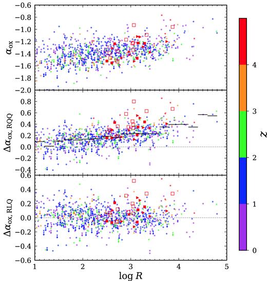
The relations between radio loudness (log R) and αox, Δαox,RQQ, and Δαox, RLQ, from top to bottom. The filled squares and triangles are from the Chandra Cycle 17 objects and archival data objects, respectively. The open squares are from Wu13. The small open circles represent the radio-loud and radio-intermediate objects in the full sample of Miller11 that are detected in X-rays, while the downward arrows have only X-ray upper limits. The dashed lines label the positions of Δαox = 0. The thick black lines in the middle panel are the mean Δαox,RQQ values for the Miller11 RLQs in log R bins (Δlog R = 0.2 per bin). All symbols are colour-coded based on their redshifts using the colour bar on the right-hand side.
We further compared the Δαox distribution of the flux-limited sample (see Section 2) with that of their low-z counterparts using histograms. We thus define a flux-limited (mi ≤ 20.26) comparison sample of HRLQs at z < 4 that is a subset of the full sample of RLQs in Miller11. The high-z and low-z samples contain 24 and 311 objects, with median redshifts of 4.4 and 1.3 (and interquartile ranges of [4.3, 4.7] and [0.9, 1.8]), respectively.
In addition to the flux-limit and radio-loudness cuts we have applied, we confirmed that the quasars in the low-z sample show comparably strong emission lines to those in the high-z sample (i.e. they are largely free from strong boosted non-thermal continuum emission in the optical/UV; see Fig. 3). We first matched the low-z sample to the DR7 quasar property catalogue (Shen et al. 2011) and checked the rest-frame equivalent widths (REWs) of Hβ, Mg ii, and C iv. 187 quasars in the low-z sample are included in the DR7 quasar property catalogue; all of them have at least one emission line (of the three we checked) that has REW > 5 Å. We also visually inspected the SDSS spectra of the 214 low-z quasars within the SDSS quasar catalogue DR14 (Pâris et al. 2018), and almost all of them show strong emission lines. To demonstrate the similarly strong emission lines in the high-z and low-z samples, we create composite SDSS spectra for the HRLQs in four redshift bins (quasars at z < 0.5 are discarded due to their largely different rest-frame wavelength ranges) and show them in Fig. 6. To create these composite spectra, each spectrum was first shifted to its rest frame and normalized to some continuum window (e.g. Vanden Berk et al. 2001), and then the median flux in each wavelength bin was calculated. It is apparent from the significant overlapping in Fig. 6 that the composite spectra of HRLQs in the different redshift bins match very well, especially in the sense that all of them show comparably strong emission lines. In Fig. 6, we also show the composite median spectrum of quasars that are detected in the FIRST survey and have f1.4 GHz ≥ 2 mJy for comparison (Kimball et al. 2011).

The composite SDSS spectra of HRLQs in different redshift bins. The quasars in bins of z = 0.5–1.0, 1.0–2.0, and 2.0–4.0 are from Miller11, and the quasars in the bin of z = 4.0–5.5 are from this paper. The grey curve (vertically shifted) is a composite spectrum of SDSS quasars that have radio counterparts with f1.4 GHz ≥ 2 mJy (Kimball et al. 2011). The composite spectra of HRLQs in different redshift bins match so well that it is hard to notice the overlapping (except that the z = 4.0–5.5 quasars suffer more severe absorption below the Lyman limit). The strengths of emission lines do not have an apparent dependence on redshift.
The histograms of Δαox,RQQ and Δαox,RLQ for the two samples are shown in Fig. 7, where the low-z sample contains upper limits as some HRLQs from Miller11 were not detected in X-rays. The distributions for the high-z and low-z samples are visually different, with not only their peaks differing by ≈0.1, but also their distributions spanning different ranges, in both panels. From the histograms of Δαox,RLQ, the HRLQs at z < 4 do not show an apparent deviation from the |$L_{2\rm \,\,keV}$|-|$L_{2500\rm~{\mathring{\rm A} }}$|-|$L_{5\rm \,\,GHz}$| relation that is derived from their parent population of general RLQs. However, HRLQs at z > 4 do not follow this relation well and have an excess of X-ray emission compared with the low-redshift sample.
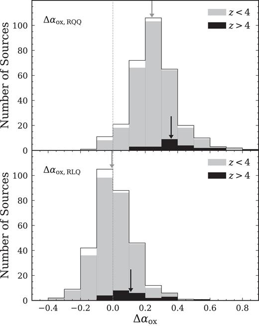
The histograms of Δαox, RQQ (top) and Δαox,RLQ (bottom) for the full-sample objects in Miller11 with log R > 2.5, z < 4, and mi ≤ 20.26. The grey and open histograms are for X-ray detected and undetected objects in the z < 4 sample, respectively. The HRLQs at z > 4 are plotted in black. The downward arrows indicate the medians of the Δαox distributions of the two redshift bins.
4.2 Quantitative statistical tests
Since there are upper limits21 in our comparison sample, to quantify the statistical significance of the difference in the Δαox distributions of the two samples, we use the Peto-Prentice test that is implemented in the Astronomy Survival Analysis Package22 to perform two-sample tests. The test shows a 4.56σ (p = 2.56 × 10⁻⁶)23 difference for the Δαox,RQQ distributions and a 4.07σ (p = 2.35 × 10⁻⁵) difference for the Δαox,RLQ distributions, both of which are better than the corresponding statistical significances measured by Wu13. Furthermore, while the statistical test results of Wu13 should be considered as suggestive (due to their incomplete X-ray coverage), our results can be accepted more formally.
The majority of the high-z sample that has multifrequency data in the radio band is flat-spectrum (αr > −0.5) objects (see Table 5). We thus performed another statistical test on the subsets of confirmed flat-spectrum quasars selected from the high-z and low-z samples. The differences of the high-z subset (17 objects) and low-z subset (100 objects) are 4.18σ (p = 1.46 × 10⁻⁵) and 3.18σ (p = 7.36 × 10⁻⁴) for the distributions of Δαox,RQQ and Δαox,RLQ, respectively. We performed a Monte Carlo simulation by randomly selecting 17 and 100 objects from the flux-limited high-z (24 objects) and low-z (311 objects) samples and running statistical tests on these sub-samples. The statistical significance typically drops by ≈1σ compared with that of the flux-limited sample; we conclude that the smaller statistical significance resulting from the flat-spectrum sub-sample is mainly caused by the smaller sample size, rather than any strong systematic difference in the degree of high-z enhancement.
Another factor that inevitably affects our statistical tests and all other such tests in the literature is the uncertainties of αox and Δαox, including contributions from flux measurement errors and intrinsic quasar variability (since the multiwavelength data have not been simultaneously obtained). The uncertainties of the X-ray fluxes are in the range of 6 per cent–30 per cent (e.g. see Table 3); the flux errors in the optical (|$\sigma _{m_i}\lesssim 0.03$| mag) and radio (σrms ≲ 0.15 mJy) are negligible compared with those for the X-rays. Since the overall variability (in X-rays and optical) dominates the uncertainties, we adopted a typical value of 20 per cent for uncertainties due to flux errors in X-rays. We take a magnitude of 25 per cent for the variability in the X-ray band (e.g. Gibson & Brandt 2012) and a magnitude of 25 per cent for the variability in the optical/UV (considering our sample contains the most-luminous quasars and RLQs are usually more variable than RQQs, e.g. Vanden Berk et al. 2004; MacLeod et al. 2010). We thus assign a typical value of 0.06 as the uncertainties on αox, which is equivalent to ≈43 per cent uncertainties on the amount of X-ray enhancement. Both measurement errors and variability are random uncertainties instead of systematic biases, and they thus broaden the Δαox distributions with the centres unchanged. The Peto-Prentice tests we performed in the analyses above compare, in fact, the broadened distributions instead of the true distributions. One of the consequences is that the power of the statistical tests is reduced by the ‘smearing’ effect of the uncertainties. In another words, if we had performed coordinated multiwavelength observations using telescopes powerful enough to ignore the measurement errors, the statistical significance would be even higher. We confirmed the effects of the uncertainties on αox on two-sample tests using Monte Carlo simulations. We also confirmed the even higher statistical significance of the ‘true’ distribution using Bayesian modelling, marginalizing out the uncertainties of αox. See Appendix B for details on the simulation and modelling process. We note that the simulation can indicate the direction of the effects of uncertainties while we are not sure whether a quantitative correction to the statistical significance is well justified or not, and the modelling analysis depends on assumptions (e.g. the Gaussian assumption, the magnitudes of the uncertainties, and priors). We thus conservatively quote the results of the statistical tests using the observed data, following the standard practice in the literature.
Among the seven objects (excluding SDSS J091316.55+591921.6) in Table 5 that are outside the flux-limited sample, three objects have less X-ray emission than predicted from the |$L_{2 \rm keV}$|-L2500Å-|$L_{5\rm GHz}$| relation of low-z RLQs (negative Δαox,RLQ values). In comparison, only four out of 24 objects in the flux-limited sample show this deficit of X-ray emission. Since our multiwavelength data are not simultaneous, variability with larger amplitude for fainter objects may generally cause larger scatter of αox. We cannot conclude from the available data that the X-ray enhancement disappears in the optically faint regime. We will need complete X-ray coverage of optically fainter HRLQs at z > 4 to improve understanding of this matter (see Section 5.3).
4.3 The amount of X-ray enhancement
We quantify the typical amount of X-ray enhancement for the high-z sample relative to the low-z sample using the difference of the medians of their Δαox distributions. The medians were calculated using the Kaplan–Meier estimator of the cumulative distribution function that can cope with upper limits in data. We describe the relevant methodology in Appendix C. The medians of Δαox,RQQ for the high-redshift and low-redshift samples are 0.37 ± 0.03 and 0.24 ± 0.01, respectively. The medians of Δαox,RLQ for the high-redshift and low-redshift samples are 0.11 ± 0.03 and 0.01 ± 0.02, respectively. The uncertainties here are estimated using bootstrapping (see the method in Appendix C). These medians are also plotted in Fig. 7 as downward arrows. The difference of the medians of the Δαox,RLQ distributions is 0.11 ± 0.04, and thus the X-ray luminosities of the HRLQs at z > 4 are typically |$1.9^{+0.5}_{-0.4}$| times those of their low-redshift counterparts. In addition to the median factor of X-ray enhancement, we also calculate the interquartile range from the Δαox,RLQ distribution of the high-z sample, which is [0.04, 0.21] and corresponds to a factor of X-ray enhancement in the range of [1.3, 3.5]. At the extremes, some objects show no X-ray enhancement while others show an enhancement by a factor of 5–25 (see Table 5).
The factor of |$1.9^{+0.5}_{-0.4}$| X-ray enhancement is somewhat smaller than but consistent with the estimation in Wu13, who found a factor of ≈3 by comparing the means of Δαox. We thus calculate the factor of X-ray enhancement using the median statistic and the 12 HRLQs that were used by Wu13 (mi < 20) resulting in a factor of |$2.6_{-1.0}^{+2.0}$|. Therefore, any apparent difference of X-ray enhancement factor is mainly caused by the large scatter due to the small sample size of Wu13 and partly by the statistic used.
We here point out one potential Malmquist-type bias (e.g. Lauer et al. 2007) that could diminish the X-ray enhancement of the high-redshift sample compared with the low-redshift sample. A larger fraction of the high-z sample is near the optical flux limit (mi = 20.26) than the low-z sample; if the optical luminosity function is steep, a large fraction of the HRLQs that are near the flux limit have, intrinsically, a dim X-ray flux. We thus select another low-z HRLQ sample with |$\log L_{2500\rm~{\mathring{\rm A} }}\gt 30.57$|, which is the minimum optical/UV luminosity of the high-z sample. The resulting low-z sample has a size of 165. We found that the X-ray enhancement of the high-z sample is a factor of |$2.0_{-0.4}^{+0.5}$|, which means this selection effect, if it exists, probably does not significantly affect our results.
4.4 HRLQs at 3 < z < 4
Wu13 performed two-sample tests on HRLQs in different redshift bins below z = 4 using the RLQs of Miller11 and found an apparent X-ray enhancement also exists at z ≈ 3. Specifically, the Δαox distributions of HRLQs at 3 < z < 4 differ from those of z < 3 HRLQs at a ≈5σ level. We thus select 3 < z < 4 HRLQs from the full RLQ sample and quantify their typical factor of X-ray enhancement relative to HRLQs at z < 3 using the same consistent method described in the previous section. We have applied an optical flux cut determined by the faintest HRLQ at 3 < z < 4 (mi = 20.38). The sample sizes (median redshifts) are 16 (z = 3.4) and 304 (z = 1.3) for 3 < z < 4 HRLQs and z < 3 HRLQs, respectively. We estimated the medians of Δαox,RLQ for 3 < z < 4 and z < 3 objects are 0.12 ± 0.07 and −0.01 ± 0.01. The corresponding factor of X-ray enhancement is |$2.0^{+1.1}_{-0.8}$|. The relatively larger error bars of our estimations are largely due to the small sample size at 3 < z < 4.
4.5 The spectral energy distributions
We here make another comparison between the X-ray emission of high-z and low-z HRLQs using their SEDs. We collected photometric data to construct the broad-band SEDs of our objects that cover the radio through X-ray bands from the following sources.
Radio: the 1.4 GHz flux densities are from the FIRST or NVSS surveys; the sources for 5 GHz values are the same as those described in Column (12) in Section 3.5; the 150 MHz flux densities are gathered from the GMRT 150 MHz all-sky survey (Intema et al. 2017); the flux densities at other frequencies were retrieved from the NED.
Mid-infrared: the all-sky catalogue of the Wide-field Infrared Survey Explorer (WISE; Wright et al. 2010) provides the mid-infrared fluxes. All of our objects are detected by WISE except for SDSS J083549.42+182520.0, SDSS J102107.57+220921.4, and SDSS J160528.21+272854.4.
Near-infrared: we first searched for objects in the Two Micron All Sky Survey (2MASS; Skrutskie et al. 2006). None of our objects has a 2MASS detection. We then searched objects in the UKIRT Infrared Deep Sky Survey (UKIDSS; Lawrence et al. 2007). Five objects (SDSS J030437.21+004653.5, PMN J2314+0201, SDSS J083549.42+182520.0, SDSS J153533.88+025423.3, and SDSS J222032.50 + 002537.5) have Y, J, H, and K detections, while SDSS J160528.21+272854.4 has only a J-band detection. We further searched for objects in the VISTA Hemisphere Survey (VHS; McMahon et al. 2013), where we found J-, H-, and Ks-band detections for SDSS J030437.21+004653.5, PMN J2134−0419, and SDSS J222032.50+002537.5, and an additional Y-band detection for PMN J2134−0419.
Optical: obtained from SDSS photometry (u, g, r, i, and z). The bands that are seriously affected by the Ly α forest are discarded.
X-ray: from this work.
None of our HRLQs has a counterpart in the Fermi LAT 4-Year Point Source Catalog (Acero et al. 2015), using a matching radius of 10 arcmin. The constructed SEDs of our HRLQs are shown in Fig. 8, in ascending order of RA. Also plotted in Fig. 8 is a comparison SED (grey curve) that was constructed by Wu13, using 10 HRLQs at z < 1.4 from Shang et al. (2011). These 10 low-z HRLQs were selected based on their optical/UV luminosity (log λLλ(3000Å) > 45.9), radio-loudness (2.9 < log R < 3.7), and useful X-ray data from the literature. Their SEDs were normalized at rest-frame 4215 Å, and medians for different waveband bins were calculated (see Section 5.2 of Shang et al. 2011). Following Wu13, we have normalized the comparison SED to the observed data for our HRLQs at rest-frame 2500 Å.

The broad-band SEDs for the HRLQs in this paper (in ascending order of RA) from radio to X-ray. The objects within our flux-limited sample are marked by ★ following their names. The solid purple lines show the X-ray power-law spectra with their uncertainties as dotted lines (see Column (9) in Section 3.5). The purple diamonds represent the observed-frame 2 keV. The grey curve is the composite SED for the 10 HRLQs at z < 1.4 from Shang et al. (2011) with comparable optical luminosity and radio loudness. This low-z comparison SED has been normalized to the high-z SEDs at rest-frame 2500 Å. The vertical lines indicate rest-frame 2500 Å and 2 keV.
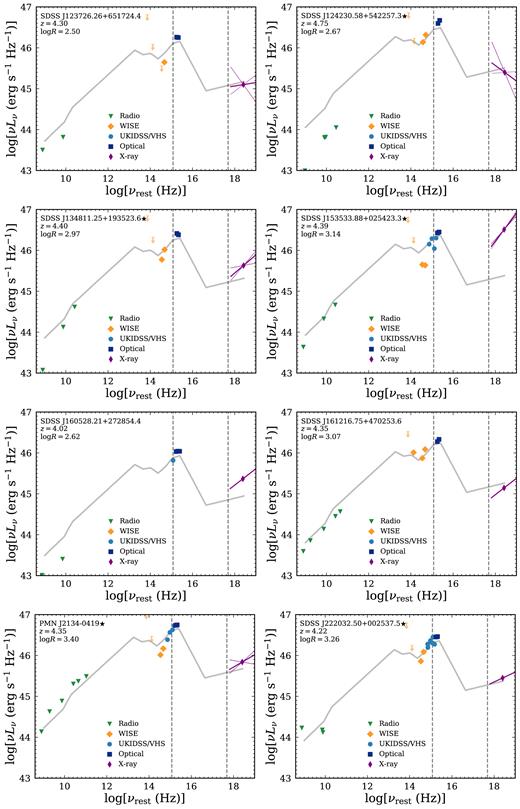
(Continued).
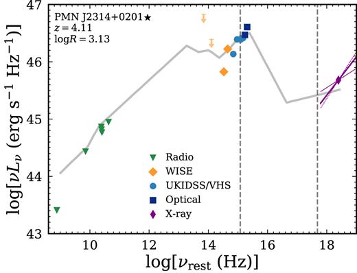
(Continued).
Five out of the 15 HRLQs have higher X-ray luminosities by a factor of ≈3–13 than that of the comparison SED, while the other 10 HRLQs have comparable X-ray luminosities with that of the comparison SED, considering the uncertainties of the X-ray luminosities. Note that the interquartile ranges of the comparison SED are 0.37 dex and 0.56 dex in the radio (5 GHz) and X-ray (2 keV) bands, respectively. Notably, SDSS J102107.57+220921.4 and SDSS J083549.42+182520.0 show a factor of ≈10 enhancement in their X-ray luminosities relative to the comparison SED; both of them were not included in our flux-limited sample due to their fainter optical fluxes, making future work that extends our systematic study to the fainter optical regime promising (see Section 5.3). Including the 17 SEDs of Wu13, half of the high-z HRLQs (16/32) show an apparent excess of X-ray emission by a factor of ∼2.5–20, compared with the low-z HRLQs with matched optical/UV luminosity and radio-loudness. Also from their SEDs, the HRLQs do not show weaker optical/UV emission, relative to their infrared emission, which means the high Δαox values indeed reflect stronger X-ray emission instead of weaker optical/UV emission. This supports the basic validity of our earlier analyses based on Δαox.
5 SUMMARY, DISCUSSION, AND FUTURE WORK
5.1 Summary
In this paper, we have tested and confirmed the X-ray enhancement of high-redshift (z > 4) HRLQs (log R > 2.5) compared with their low-redshift (z < 4) counterparts. We summarize the key points from this work:
We selected the high-redshift (z > 4) HRLQs from Wu13 and new objects from sky surveys (SDSS and FIRST) and NED. We obtained Chandra observations in Cycle 17 for six HRLQs that lacked sensitive X-ray coverage. We also retrieved archival XMM–Newton and Swift X-ray observations that cover another nine high-z HRLQs. We finally constructed an optically flux-limited sample of 24 HRLQs to mi = 20.26 that has complete sensitive X-ray coverage. See Section 2.
We analysed the X-ray data and measured HRLQ X-ray photometric properties (see Table 3). All the Chandra Cycle 17 objects were detected in X-rays. No extended structure was found in the Chandra images, including for SDSS J0813+3508, which is the only Chandra Cycle 17 object that has an extended structure in its FIRST image. See Section 3.
HRLQs at z > 4 show an apparent X-ray enhancement compared with matched HRLQs at z < 4. The Δαox (including Δαox,RQQ and Δαox,RLQ) distributions of the optically flux-limited high-z sample are significantly different (≈ 4–4.6σ) from those of the low-z sample. This result confirms the relevant result of Wu13, in a statistically stronger way and with fewer systematic uncertainties. See Section 4.2.
The typical (median) X-ray enhancement of HRLQs at z > 4 is a factor of |$1.9^{+0.5}_{-0.4}$|; this is smaller than but still consistent with the estimation of Wu13. See Section 4.3.
We constructed the radio–X-ray continuum SEDs for the HRLQs analysed in this paper, which further illustrate and support the excess of X-ray emission of high-z HRLQs compared with their low-z counterparts. See Section 4.5.
5.2 Discussion
We have confirmed the X-ray enhancement of HRLQs at z > 4 that was originally proposed by Wu13. However, we revised the typical amount of X-ray enhancement from a factor of ≈3 to ≈2. We plot the factor of X-ray enhancement using the estimates for HRLQs at z > 4 in Fig. 9. The fractional IC/CMB model that was suggested by Wu13 can still explain our results if the fraction of X-rays from the IC/CMB mechanism in HRLQs decreases accordingly. More specifically, if IC/CMB produces 3 per cent of the X-ray radiation from HRLQs at z = 1.3, a factor of ≈2 X-ray enhancement at our median redshift of z = 4.4 can be reproduced according to UCMB ∝ (1 + z)4 evolution, assuming that the high-z jets are not physically different (e.g. severely decelerated on kpc scales; Lopez et al. 2006; Volonteri et al. 2011; Marshall et al. 2018) from the low-z jets.
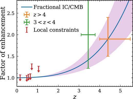
The current constraints on the evolution of the X-ray enhancement of HRLQs using the z > 4 sample from this paper and Wu13 and the 3 < z < 4 sample from Miller11. The blue curve and purple-shaded region are the prediction from the fractional IC/CMB model and its uncertainties, which are calibrated using the z > 4 redshift bin. We constrain the contribution of the IC/CMB mechanism at z = 1.3 to be ≈3 per cent, with an upper limit of ≈5 per cent. The red upper limits are the constraints from non-detections of IC/CMB-predicted γ-ray emission from low-z large-scale jets using Fermi (Meyer et al. 2015; Breiding et al. 2017; Meyer et al. 2017). See Section 5.2 for details.
We have plotted in Fig. 9 the prediction and uncertainties of our revised fractional IC/CMB model for the factor of X-ray enhancement with redshift (blue curve and purple-shaded region). The curve has the form of 1 + A[(1 + z)/(1 + 4.4)]4, which represents the combination of a non-evolving component and an evolving IC/CMB-related component. This curve is calibrated by the analysis of z > 4 HRLQs. For example, A needs to be ≈0.9 for the blue curve to match the observed enhancement of 1.9 at z = 4.4. The boundary of the shaded region is determined accordingly using the error bars of the z = 4.4 data point. The curve is consistent with the constraint from 3 < z < 4 HRLQs, which show more substantial uncertainties due to limited sample size. A larger sample will help to provide tighter constraints on the X-ray enhancement of HRLQs in this redshift bin. Note that at z ≈ 1 and z ≈ 2 the expected X-ray enhancements are only factors of 1.02 and 1.09, with upper limits of 1.03 and 1.13, respectively.
Recall that the quasars with high-resolution Chandra observations in our sample do not show any extended structure in their X-ray images, and the jet-linked X-ray emission is most probably from regions smaller than a few kpc. The high-z large-scale X-ray jets (if they exist) must lie below the flux limits of our X-ray observations and are much dimmer than the core region, in contrast with the prediction of the most-straightforward IC/CMB model under the assumption that the radio fluxes of the jets relative to those of the cores do not evolve with redshift (Schwartz 2002; also see Bassett et al. 2004; Lopez et al. 2006; Miller11). Either a high-energy synchrotron-emitting electron population or an improved understanding of quasar jets is needed to explain the commonly detected large-scale X-ray jets of low-z quasars.
The IC/CMB-dominated model for the X-ray emission of large-scale quasar jets predicts significant radiation in the high-energy γ-ray band (e.g. Tavecchio et al. 2004), and Fermi observations have thus been suggested to be used to test the IC/CMB model (e.g. Dermer & Atoyan 2004). The first such test was performed by Meyer & Georganopoulos (2014) on the large-scale jet of 3C 273 and their results disfavour the IC/CMB-dominated model. We here compare the constraints on the IC/CMB X-ray emission from our high-z quasars with the constraints from z ≈ 0.1–1 large-scale jets, which are shown as upper limits in Fig. 9. The six upper limits are the following: 1.068 (3C 273, z = 0.160; Meyer et al. 2015), 1.095 (PKS 0637−752, z = 0.650; Meyer et al. 2017), 1.055 (PKS 2209+080, z = 0.480), 1.082 (PKS 1136−135, z = 0.560), 1.324 (PKS 1354+195, z = 0.720), and 1.269 (PKS 1229−021, z = 1.05; Breiding et al. 2017). Following Meyer et al. (2015), we have assumed the ‘angle-averaged’ jet-linked X-ray emission from those low-z RLQs is dominated by large-scale jets, after correcting for the beaming effect of the radiation from the cores. We calculated the ratio between the upper limit from the Fermi data and the predicted IC/CMB γ-rays, which is equivalent to the upper limit on the fraction of IC/CMB X-ray emission to total jet-linked X-rays. Since the literature has divided the Fermi bandpass into multiple sub-bands, we have chosen the band giving the most-stringent constraint.
Note that early X-ray studies using representative samples of moderately radio-loud to highly radio-loud (1 ≲ log R ≲ 4) quasars at z > 4 (e.g. Bassett et al. 2004; Lopez et al. 2006; Wu13) have argued against the scenario where the IC/CMB mechanism plays a dominant role in the jet-linked X-ray emission from these high-redshift objects (e.g. Schwartz 2002). In addition, Miller11 found no evidence supporting an apparent redshift dependence of X-ray properties in their large-sample (607 objects) study of RLQs that spans 0 < z < 5 and 1 < log R < 5.
Indeed, considering the X-ray jets of PKS 0637−752 (z = 0.650, |$L_{2-10\ \rm keV}\approx 4\times 10^{44}$| erg s−1; Schwartz et al. 2000) and B3 0727 + 409 (z = 2.5, |$L_{2-10\ \rm keV}\approx 6\times 10^{44}$| erg s−1; Simionescu et al. 2016), if the IC/CMB model were responsible for their X-ray emission, their analogues at z ≈ 4.4 would have |$L_{2-10\ \rm keV}\approx 5\times 10^{46}$| erg s−1 and |$L_{2-10\ \rm keV}\approx 3\times 10^{45}$| erg s−1, both of which would outshine their cores in X-rays. However, X-ray observations of RLQs at z > 4 do not support this prediction (e.g. Bassett et al. 2004; Lopez et al. 2006; Saez et al. 2011; Miller et al. 2011; Wu13). 24 Note that the X-ray luminosities of the few resolved z > 4 kpc-scale jets are only a few per cent that of the quasar cores (e.g. Yuan et al. 2003; Cheung et al. 2012), consistent with the results for low-z jets.
McKeough et al. (2016) investigated the redshift dependence of the X-ray-to-radio flux ratios (αxr) of 11 quasars and found that the z > 3 quasars have marginally stronger X-ray emission relative to the z < 3 quasars in their sample. Marshall et al. (2018) studied the αrx distribution of 56 quasar jets at z ≲ 2 and found weak redshift dependence with their 0.95 < z < 2.05 sub-sample showing marginally larger X-ray flux densities relative to that of radio than their 0.55 < z < 0.95 sub-sample. Their results disfavour the scenario where the IC/CMB mechanism dominates the jets’ X-ray emission (without changing the properties of high-z jets) and are consistent with our previous result from z > 4 RLQs.
Wu13 also discussed another possible cause of the X-ray enhancements in which the photon field of the host galaxy inverse-Compton scatters off the relativistic electrons in the jets. This mechanism requires the host galaxies at high redshifts to have enhanced star-formation activity that produces dense infrared photon fields (e.g. Wang et al. 2011; Mor et al. 2012; Netzer et al. 2014). Our results can still be explained by this scenario. While the cosmological evolution of the CMB energy density can be easily predicted, the evolution of the star-forming activity of the hosts of quasars with powerful relativistic jets at different redshifts has not been established (e.g. Archibald et al. 2001). However, if future X-ray studies of HRLQs that extend to z ≈ 0.5–4 detect any deviation from the prediction of the blue curve in Fig. 9 and disfavour the fractional IC/CMB model, alternative models like this will gain more credit.
Ajello et al. (2009) found that the number density of flat-spectrum radio quasars (FSRQs) selected by the Swift/Burst Alert Telescope (BAT; in hard X-rays) has a peak at a notably high redshift of z ≈ 3–4. The interpretation of such a number-density peak can be affected by the X-ray luminosity enhancement of HRLQs at z > 4 we confirmed here. Qualitatively, this X-ray enhancement might cause high-z HRLQs to be more easily picked up by Swift/BAT, and their apparent peak in number density will correspondingly be biased toward a higher redshift. A quantitative discussion of this issue is beyond the scope of this paper.
5.3 Future work
There are several ways the results in this work might be productively extended. First, the sample statistics of the z > 4 HRLQs could be improved by future X-ray observations of the additional objects listed in Table 2. Several objects in Table 2 have already been scheduled for Chandra observations, and a Chandra snapshot survey of the remaining objects would extend complete X-ray coverage to an optically flux-limited sample reaching mi = 21 with a size of 37. With this larger sample size, the level of X-ray enhancement of z > 4 HRLQs could be better constrained.
Furthermore, one could now substantially enlarge the sample of HRLQs at z < 4 with sensitive X-ray coverage via systematic archival data mining. The Miller11 sample used for our z < 4 comparisons here was largely based on SDSS Data Release 5 (DR5) from 2007 (e.g. Schneider et al. 2007), and it utilized X-ray coverage from Chandra, XMM–Newton, and ROSAT. Over the past decade, more than 450 000 new quasars have been spectroscopically identified by the SDSS (e.g. Pâris et al. 2018), including many new HRLQs at z ≈ 0.5–4. Furthermore, the sizes of the Chandra and XMM–Newton archives have grown substantially since the work of Miller11, and more sensitive radio data have been gathered in the SDSS footprint (e.g. via the ongoing VLA Sky Survey25). Systematic archival X-ray analyses of these new z ≈ 0.5–4 HRLQs should allow more precise measurements of the factor of X-ray enhancement versus redshift (see Fig. 9), thereby testing and quantifying the fractional IC/CMB model.
Finally, alternative explanations of the observed X-ray enhancement should also be explored. For example, ALMA measurements of star-formation rates for z > 4 HRLQ hosts could test if their star formation is sufficiently elevated to drive the X-ray enhancement via a stronger host seed photon field (see Section 1).
ACKNOWLEDGEMENTS
We thank M. Ajello, D. P. Schneider, and W. M. Yi for helpful discussions. We thank the referee for helpful comments. SFZ and WNB acknowledge support from the Penn State ACIS Instrument Team Contract SV4-74018 (issued by the Chandra X-ray Center, which is operated by the Smithsonian Astrophysical Observatory for and on behalf of NASA under contract NAS8-03060) and CXC grant AR8-19011X. The Chandra Guaranteed Time Observations (GTO) for some of the quasars studied herein were selected by the ACIS Instrument Principal Investigator, Gordon P. Garmire, currently of the Huntingdon Institute for X-ray Astronomy, LLC, which is under contract to the Smithsonian Astrophysical Observatory via Contract SV2-82024.
This research has made use of data and/or software provided by the High Energy Astrophysics Science Archive Research Center (HEASARC), which is a service of the Astrophysics Science Division at NASA/GSFC and the High Energy Astrophysics Division of the Smithsonian Astrophysical Observatory. This research has made use of the NASA/IPAC Extragalactic Database (NED) which is operated by the Jet Propulsion Laboratory, California Institute of Technology, under contract with the National Aeronautics and Space Administration. Funding for the Sloan Digital Sky Survey IV has been provided by the Alfred P. Sloan Foundation, the U.S. Department of Energy Office of Science, and the Participating Institutions. SDSS-IV acknowledge support and resources from the Center for High-Performance Computing at the University of Utah. The SDSS web site is www.sdss.org. SDSS-IV is managed by the Astrophysical Research Consortium for the Participating Institutions of the SDSS Collaboration including the Brazillian Participation Group, the Carnegie Institution for Science, Carnegie Mellon University, the Chilean Participation Group, the French Participation Group, Harvard-Smithsonian Center for Astrophysics, Instituto de Astrofísica de Canarias, The Johns Hopkins University, Kavli Institute for the Physics and Mathematics of the University (IPMU) / University of Tokyo, Lawrence Berkeley National Laboratory, Leibniz Institude für Astrophysik Potsdam (AIP), Max-Planck-Institut für Astronomie (MPIA Heidelberg), Max-Planck-Institut für Astrophysik (MPA Garching), Max-Planck-Institut für Extraterrestrische Physick (MPE), National Astronomical Observatories of China, New Mexico State University, New York University, University of Notre Dame, Observatário Nacional / MCTI, The Ohio State University, Pennsylvania State University, Shanghai Astronomical Observatory, United Kingdom Participation Group, Universidad Nacional Autónoma de México, University of Arizona, University of Colorado Boulder, University of Oxford, University of Portsmouth, University of Utah, University of Virginia, University of Washington, University of Wisconsin, Vanderbilt University, and Yale University.
Footnotes
Use of the terms ‘radio-loud AGN’ and ‘radio-quiet AGN’ is sometimes inappropriate; e.g. when the optical AGN continuum is obscured or when the radio continuum has a strong contribution from non-jet emission (e.g. Padovani 2017). However, for the powerful type 1 quasars with strong jets under study here, use of this terminology is appropriate (Padovani, private communication).
We hereafter refer to objects at z > 4 as high-redshift/high-z objects and objects at z < 4 as low-redshift/low-z objects.
SDSS J003126.79+150739.5 and SDSS J123142.17+381658.9 are in Table 2 of Wu13. However, they do not satisfy the criterion of log R > 2.5 if we take their rest-frame 2500 Å luminosities from spectral fitting (Shen et al. 2011) instead of mi. We have thus revised the Wu13 sample from 28 objects to 26 objects.
SDSS J003126.79+150739.5 and SDSS J123142.17+381658.9 were also awarded Chandra time in Cycle 17. We analyse their X-ray data and report the results in Table 3, but will not show them in the figures or include them in the statistical tests.
The typical radio fluxes of the high-z HRLQs are f1.4GHz ≥ 20 mJy.
We used a larger background region to enclose more background events in extracting background spectra.
Including both aperture-corrected and uncorrected ARFs.
These two serendipitously observed HRLQs are near to the edges of the EPIC-pn CCDs, with off-axis angles of ≈15′–17′.
PB is the chance probability of observing a signal no weaker than the source counts under the null hypothesis that there is no source in the source-extraction region. Thus, it is essentially a p-value.
See http://cxc.harvard.edu/ciao/ahelp/modelflux.html and http://cxc.harvard.edu/ciao/why/pimms.html. Since we have obtained response files for all the observations, we also use modelflux with XMM–Newton and Swift data.
SDSS J003126.79 + 150739.5 with log R = 2.44 does not strictly satisfy our definition for HRLQs, but it has an even steeper effective photon index.
Miller11 quantify radio loudness using the ratio of monochromatic luminosities at rest-frame 5 GHz and 2500 Å. We have converted their values of radio loudness to the values according to our definition, assuming α = −0.5.
Note that Miller11 calculated relatively conservative 95 per cent confidence upper limits for the X-ray flux when a quasar is not detected in X-rays. Considering the 19 non-detections in the low-z sample, ≈18 are expected to be correct in the sense that the flux is actually below the limit value.
Downloaded from http://astrostatistics.psu.edu/statcodes/asurv. See Feigelson & Nelson (1985).
The p-values in this section are the probabilities of the data under the null hypothesis and correspond to the significance level in one-sided tests using a standard normal distribution.
B3 0727+409 has a large-scale jet that is bright at X-ray and faint at radio, which is thought to be consistent with the prediction of IC/CMB model (Simionescu et al. 2016). However, B3 0727+409 has a core that is extremely radio-loud (log R ≈ 6), and thus its analogue at z > 4 will not be missed by our selection criterion.
Feigelson & Nelson (1985) circumvent this by providing a prescription that converts left-censored data to right-censored data.
REFERENCES
,
APPENDIX A: STATISTICAL TESTING FOR EXTENDED STRUCTURE
The Chandra Cycle 17 objects mostly have limited photon counts. It is not feasible to directly compare their images with the PSF images to check for extended X-ray jets (e.g. Wu et al. 2017). We first produced the PSF image for each observation using ray-tracing26 with a large number of simulated events. The statistical method we used is as follows.
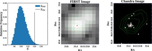
Left: The empirical distribution of S (blue histogram) calculated using simulated images of the Chandra PSF, together with the S value (vertical black line) calculated using the observed 0.5–8 keV Chandra image of SDSS J0813+3508. Centre: Radio image of SDSS J0813+3508 from FIRST at 1.4 GHz. Right: X-ray image of SDSS J0813+3508 in the 0.5–8 keV band. The red ‘×’ symbols in both the centre and right-hand panels indicate the optical position of the quasar. Contours of the radio image are plotted in both the centre and right-hand panels, where the radio surface brightness increases from 2.9 mJy beam−1 (outermost) to 12.2 mJy beam−1 (innermost) with a step size of 3.3 mJy beam−1. Even though Sobs appears marginally inconsistent with the distribution predicted by the Chandra PSF (left, p ≈ 0.011), the X-ray image (right) does not show an extended structure that corresponds to the structure in the radio image (centre).
In our calculation, we used D = 20 (i.e. the size of the patch is 10 arcsec × 10 arcsec). We found a detection for the 0.5–8 keV image of SDSS J0813+3508 with p = 0.0108, which becomes less significant (the p-value increases to p = 0.0832) after taking into account the number of tests we have performed (e.g. Conrad 2015). We then compared the radio and X-ray images of SDSS J0813+3508, and did not find extended X-ray structure that corresponds to the radio jet, as shown in Fig. A1 (centre and right). Note that the extended radio component that is ≈7 arcsec away from SDSS J0813+3508 has a peak radio flux density (11.9 mJy) that is about half that of the core (20.0 mJy). We estimated the (observed-frame 0.5–2 keV) surface brightness coincident with the extended radio component to be <1.43 × 10⁻¹⁶ er g cm−2 s−1 arcsec−2, which means that the extended jet (if it exists) must be more than 10 times dimmer than the core in X-rays. Other sources are consistent with point sources. We conclude that no statistically convincing extended structure is found in the X-ray images.
We investigated further the constraints coming from the non-detections on the relative brightness of X-ray jets. In the X-ray images, we put an artificial point source 2 arcsec (4 pixels; the typical size of the resolved X-ray jets for quasars at z > 4) away from the core and increase its intensity until it is detected with the statistical tests above. Typically 3–4 photons are needed for the artificial jets to be detected. Therefore, any X-ray jets have to be ≳ 3–25 times fainter than the cores for the Chandra Cycle 17 quasars, consistent with previous X-ray upper limits for high-z RLQs (e.g. Bassett et al. 2004; Lopez et al. 2006).
APPENDIX B: THE EFFECTS OF NON-SIMULTANEOUS DATA AND MEASUREMENT ERRORS
Since both types of uncertainties under consideration, measurement errors, and variability, are stochastic in nature, it is impossible to apply corrections to the observed data to obtain underlying ‘true’ values. The purpose of the Monte Carlo simulation is to add more fluctuations to the data and observe the consequence of the enlarged uncertainties. We created degraded samples by adding random numbers drawn from N(0, 0.062) (a Gaussian distribution with zero mean and standard deviation σ = 0.06) to the observed Δαox (only detections). The statistical significance typically drops by ∼1σ using these worsened values, which is expected because more noise will tend to wash out the differences between the two distributions.
We have drawn samples from the posterior distributions of μ and σi for Δαox,RQQ and Δαox,RLQ for both redshift bins. We plot in Fig. B1 the comparison of μ for different redshift bins. The impact of the sample size reflects itself in the concentration of the distribution: the mean of the low-z sample is better constrained than that of the high-z sample. Student’s t-tests return, practically, p = 0.0, i.e. it is almost impossible for the centres of the Δαox distributions for the different redshift bins to be consistent with each other, after considering the smearing effect of uncertainties.
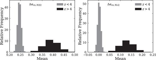
The posterior distribution of the means (also medians) of Δαox,RQQ (left) and Δαox,RLQ (right), where grey denotes the low-z sample and black denotes the high-z sample.
In addition to hypothesis testing, the modelling process above can also be used to calculate the amount of X-ray enhancement (Section 4.3). Fig. B1 (right) indicates that the Δαox,RLQ of HRLQs at z > 4 are larger than that of HRLQs at z < 4 by 0.13 ± 0.03 on average, which is consistent with the result of the Kaplan–Meier estimator.
APPENDIX C: KAPLAN–MEIER ESTIMATOR AND BOOTSTRAPPING
Some HRLQs in the Miller11 sample have only upper limits for their X-ray fluxes, which leads to the corresponding measurements of Δαox also being upper limits. Therefore, we measure the median of Δαox using the Kaplan–Meier curve (Kaplan & Meier 1958), which is a maximum-likelihood estimator of the survival function (or, equivalently, the cumulative distribution function). To justify its application to our problem, we briefly provide in the below a heuristic derivation of the Kaplan–Meier estimator based on the assumption that whether an HRLQ is detected or not in X-rays is independent of the true value of its Δαox, which is essential for the application of survival analysis (e.g. Avni et al. 1980; Wall & Jenkins 2012). The upper limits of Δαox,RQQ and Δαox,RLQ from Miller11 spread across a wide dynamic range (see Fig. 7), and thus we think this assumption is reasonable. The derivation deals with left-censored data (data with upper limits) that are common in the astronomical context, while most of the statistical literature deals with right-censored data (data with lower limits).27
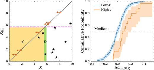
Left: The x-axis is the value of detection, and the y-axis is the limit of each observation. Upper limits are shown as leftward arrows, in contrast to detections that are shown as stars. The number of detections in the narrow green area is noted as D; the number of observations (including detections and upper limits) in the non-overlapping yellow-shaded area is noted as C−. A sub-sample is defined by the dashed purple line, under which the data points can represent the distribution of that of the complete sample on X direction if X and Xlim are independent of each other. Right: The cumulative probability distribution of Δαox,RLQ of the flux-limited samples of HRLQs at high redshift (orange) and low redshift (blue). The crossing points of the horizontal dashed lines with the curves are medians.
This derivation is motivated by that of the C− method in Lynden-Bell (1971), based on the similarity between their mathematical forms. The estimator of the survival function for right-censored data can be easily derived from a plot that is similar to Fig. C1 (left), where the detections are in the top-left triangle of the Xlim-X plane and lower limits are rightward arrows on the diagonal. See Feigelson & Nelson (1985) and Schmitt (1985) for a complete discussion on astronomical applications of the Kaplan–Meier estimator and Avni et al. (1980) for a different algorithm that works with singly censored astronomical data.
