EasyCritics – I. Efficient detection of strongly lensing galaxy groups and clusters in wide-field surveys

Stapelberg, Sebastian; Carrasco, Mauricio; Maturi, Matteo

doi:10.1093/mnras/sty2784

Abstract

We present EasyCritics, an algorithm to detect strongly lensing groups and clusters in wide-field surveys without relying on a direct recognition of arcs. EasyCritics assumes that light traces mass in order to predict the most likely locations of critical curves from the observed fluxes of luminous red early-type galaxies in the line of sight. The positions, redshifts, and fluxes of these galaxies constrain the idealized gravitational lensing potential as a function of source redshift up to five free parameters, which are calibrated on few known lenses. From the lensing potential, EasyCritics derives the critical curves for a given, representative source redshift. The code is highly parallelized, uses fast Fourier methods and, optionally, GPU acceleration in order to process large data sets efficiently. The search of a |$\smash{1 \, \mathrm{deg}^2}$| field of view requires less than 1 min on a modern quad-core CPU, when using a pixel resolution of 0.25 arcsec px⁻¹. In this first part of a paper series on EasyCritics, we describe the main underlying concepts and present a first demonstration on data from the Canada–France–Hawaii-Telescope Lensing Survey. We show that EasyCritics is able to identify known group- and cluster-scale lenses, including a cluster with two giant arc candidates that were previously missed by automated arc detectors.

gravitational lensing: strong, methods: data analysis, galaxies: clusters: general, galaxies: elliptical and lenticular, cD, galaxies: groups: general

1 INTRODUCTION

Gravitational lensing by galaxy clusters has become a powerful tool for studying the dark Universe. Strong and weak lensing signatures provide the most robust observational constraints on the projected mass distribution in clusters (e.g. Cacciato et al. 2006; Limousin et al. 2007; Merten et al. 2009). The cluster mass function and profiles are sensitive to the late time evolution of cosmic structures and thus offer insights into fundamental questions of cosmology, such as the origin of the cosmic acceleration (Voit 2005; Allen, Evrard & Mantz 2011).

In the dense core regions of massive groups and clusters, lensing unfolds its strong regime, where multiple images of a background source can be formed. For extended sources, these images are highly distorted and magnified, which causes them to appear in the form of luminous arcs. The analysis of arcs and multiple images allows us to probe the inner cluster structure with minimal biases (e.g. Meneghetti et al. 2013), to measure the Hubble constant (e.g. Grillo et al. 2018; Vega-Ferrero et al. 2018) and to test cosmological models with giant arc statistics (e.g. Bartelmann et al. 1998).

Intriguingly, the statistics of giant arcs are observed to be in conflict with theoretical expectations. For nearly two decades, ΛCDM cosmological simulations have underestimated both the abundance (Bartelmann et al. 1998; Gladders et al. 2003; Li et al. 2006; Fedeli et al. 2008; Horesh et al. 2011; Bayliss 2012) and the mean radii (e.g. Broadhurst & Barkana 2008; Zitrin et al. 2012a) of giant arcs by differing amounts. Although considerable progress has been made in refining simulations with improved lens and source models, the precise levels and origins of these discrepancies are still not well understood (Meneghetti et al. 2013; Boldrin et al. 2016). One of the major reasons for this uncertain picture is the limited sizes of available data sets, which so far appear insufficient for a solid comparison of theory with observations.

At present, the largest homogeneous samples of giant arcs comprise a few hundred exemplars only. A significant rise in the rate of detections, however, is expected with the next generation of wide-field surveys, carried out with the ESA Euclid space mission (Laureijs et al. 2011) and the Large Synoptic Survey Telescope (LSST Science Collaboration 2009). The latter promises order-of-magnitude increases in the number of observed arcs (Boldrin et al. 2012), opening exciting prospects for the use of giant arcs as a competitive cosmological probe.

However, the reliable identification of strong lensing events within large image material remains a significant challenge. Recent blind searches have focused on crowdsourced visual inspection (e.g. Marshall et al. 2016) and automated arc-finding algorithms (e.g. Lenzen, Schindler & Scherzer 2004; Horesh et al. 2005; Alard 2006; Seidel & Bartelmann 2007; More et al. 2012; Xu et al. 2016). Although many new arc candidates were discovered, especially around single galaxies, both approaches face some limitations. Visual inspection generally lacks an objective definition of arcs. Moreover, it does not allow for a straightforward repetition of the analysis with new selection criteria; and, in addition, it is highly time consuming. In order to remain feasible, the efforts of increasingly large communities of trained volunteers are required (e.g. Marshall et al. 2016; More et al. 2016). Automated arc detectors, on the other hand, mostly suffer from a high contamination with spurious detections – at least in the case of searches on group and cluster scales, where the features of interest can have complex morphologies. As a result, a manual validation of up to thousands of candidates per square degree is required none the less (Maturi, Mizera & Seidel 2014).

In order to alleviate the human bottleneck in lens detection, increasing interest has lately been devoted to machine learning methods (e.g. Bom et al. 2017; Jacobs et al. 2017). None the less, there are good reasons to investigate alternative strategies for lens detection, as well. Arc-based searches are naturally affected by ambiguities due to the inherent similarity of arcs with several other, commonly observed features.¹ The secure identification of arcs thus requires a subsequent spectroscopic redshift measurement. For this, the candidate samples need to be sufficiently pure to optimize the follow-up efficiency. An effective decontamination of candidate samples can only be achieved at high costs, involving the use of increasingly complex – and less physically understood – search patterns or the exhaustion of time and human resources. Complementary to the existing approaches, however, a pre-selection of targets for arc searches, based on additional, independent indicators of the presence of strongly lensing structures, may have the potential to remove a significant part of the aforementioned ambiguities with minimal effort and based on simple physical arguments.

Here, we present a method that identifies group- and cluster-scale strong lenses by their own optical characteristics rather than by their effect on background images. We introduce the EasyCritics algorithm, which predicts the locations of critical curves based on the spatial distribution of early-type luminous red galaxies (LRGs) observed in the line of sight. Under the assumption that this distribution follows the underlying matter field, EasyCritics develops an idealized model of the line-of-sight mass density distribution, which requires only five free parameters and is used to predict the lensing potential. For a given source redshift, EasyCritics then produces maps and catalogues of the resulting critical curves, which can be used to pre-select targets for a subsequent inspection with conventional methods. The pre-selection with EasyCritics promises (1) a significant increase in efficiency compared to visual inspection methods; (2) a significant increase in purity compared to existing automated methods; (3) a quantitative criterion for rating the likelihood of detections; and (4) a first estimate of the strong lensing properties, such as the sizes and orientations of the critical curves.

The underlying assumption that light traces mass (LTM) is well tested over a wide range of scales (e.g. Bahcall & Kulier 2014; Zitrin et al. 2015). Early-type LRGs, in particular, have been recognized as distinguished probes of the underlying density field (e.g. Gavazzi et al. 2004; Zheng et al. 2009; Zitrin et al. 2012b; Wong et al. 2013). In the context of lens modelling, the LTM assumption is routinely used for the reconstruction and prediction of multiple images in massive clusters (e.g. Limousin et al.2007,2012; Zitrin et al. 2009, 2011b; Richard et al. 2014; Ishigaki et al. 2015; Jauzac et al. 2015; Kawamata et al. 2016; Caminha et al. 2017). So far, however, the LTM-based analysis of lensing has primarily focused on fitting the properties of individual, known lenses. In contrast, EasyCritics blindly models the foreground structures over an entire line of sight and throughout large celestial regions – not only for predefined, isolated galaxy clusters. The galaxies to be used are determined automatically according to their luminosity function and for different redshift bins. In doing so, EasyCritics combines the lens modelling approach described by Zitrin et al. (2009) and the arc-free analysis by Zitrin et al. (2012b) with the LRG-based lens detection by Wong et al. (2013) and Ammons et al. (2014). Due to the much larger data sets at hand, the mathematical approach and numerical implementation were changed in order to achieve higher computational performances.

This is the first of a series of papers devoted to EasyCritics. In this work, we describe the underlying concepts and methods, and demonstrate their feasibility by showing a few preliminary examples of the application of EasyCritics to data from the Canada–France–Hawaii-Telescope Lensing survey (CFHTLenS; Heymans et al. 2012; Erben et al. 2013). In two forthcoming papers, we will furthermore provide a full statistical description of the purity and completeness, the positive detections, and their lensing properties; and a comparison of the latter with other studies – using both observational (Carrasco et al. 2018, in preparation) and simulated data.

The paper is organized as follows. Section 2 summarizes the input observables and pre-processing steps. Section 3 gives an outline of the LTM model, as we propose it, and Section 4 proceeds with our description of lensing. In Section 5, we then discuss details of the numerical implementation, before we conclude this work with the application examples in Section 6.

2 OBSERVABLES AND GALAXY SELECTION

EasyCritics takes as input a galaxy catalogue, containing the coordinates |$\boldsymbol{\theta }$|⁠, photometric or spectroscopic redshifts |$z$| and red²-band fluxes F of all early-type³ (E/S0) galaxies observed. The fluxes are converted to intrinsic luminosities L using the redshift information and the luminosity distance for a given background cosmological model.

EasyCritics selects all galaxies from a user-defined redshift interval. In this study, we restrict ourselves to the range:

\begin{eqnarray*} 0.2 \lesssim z \lesssim 0.9, \end{eqnarray*}

(1)

which is motivated by the results of previous studies of the redshift distribution of strong lenses with large arcs (e.g. Bayliss et al. 2011a; Bayliss 2012; Carrasco et al. 2017). If necessary, the range can be restricted further, so as to ensure that the characteristic magnitudes remain sufficiently below the respective limiting magnitudes and that the photometric redshift uncertainties are reliable.

The galaxy redshifts are binned, with the size of each bin set to twice the median photometric measurement uncertainty Δ|$z$| of the given input data. The position of each bin is then set to the average redshift of the galaxies it contains. For a future implementation, we intend to take into account the whole redshift probability density distribution by accordingly distributing the contribution of each galaxy over multiple bins.

For each redshift bin, we select only the brightest galaxies with red-band absolute magnitudes below

\begin{eqnarray*} M \lesssim M_{\star } + 2. \end{eqnarray*}

(2)

Here, M_⋆ denotes the characteristic magnitude that we obtain by fitting the Schechter luminosity function (Schechter 1976). This selection removes galaxies with large photometric uncertainties and would yield insignificant or even spurious contributions to the mass estimate.

3 MASS MODEL

EasyCritics uses the distribution of light from LRGs for a blind, automated identification and modelling of strongly lensing structures. These structures are distributed over a wide range in redshift and their strong lensing signatures may be perturbed significantly by the foreground interlopers present within the line of sight (e.g. Wambsganss, Bode & Ostriker 2005; King & Corless 2007; Puchwein & Hilbert 2009; Wong et al. 2013; Bayliss et al. 2014). For this reason, we include all galaxies, selected as discussed in Section 2, within the considered light cone. In this section, we discuss our mass model based on the LTM approach.

3.1 Stacked mass sheets

We introduce mass sheets |$\smash{\Sigma ^{(k)}}$||$(k \in \mathbb{N})$| at all redshift bins |$\smash{z^{(k)}}$| (cf. Fig. 1, left). The surface density distribution on each sheet is modelled based on the LRGs belonging to the respective bin. In our derivation, we assume that there is only one dominant group- or cluster-scale lens within the line of sight, while the remaining structures add weak and uncorrelated local perturbations only. The angular separation of the lenses at different redshifts is assumed to be large enough for their deflections to be effectively independent. This assumption allows us to neglect the lens–lens coupling between the sheets and is justified by the low probability of having chance alignments of large objects, such as the groups and clusters we are interested in (e.g. Schneider 2014, and references therein). However, in the rare situation that such alignments are encountered, EasyCritics would detect the lenses anyway unless their ability to form a critical curve depends on the higher order interactions.

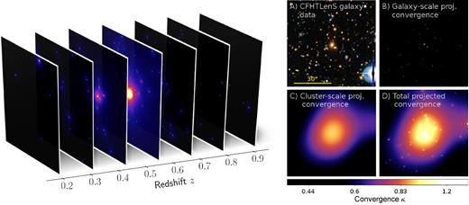
$Blind identification and modelling of overdense line-of-sight structures based on LRGs, illustrated for a region centred on a cluster-scale detection. Left: Surface density distributions $\smash{\Sigma ^{(k)}}$ of the various sheets distributed along the line of sight, in arbitrary units. Right: CFHTLenS i′r′g′-composite image (A) and line-of-sight projected maps of the predicted convergence at different levels of the modelling procedure (B–D). Shown are (B) the projected convergence $\smash{\bar{\kappa }_{\mathrm{gal}}}$ of the galaxies only, (C) the resulting projected convergence $\smash{\bar{\kappa }_{\mathrm{clus}}}$ of cluster-scale matter, and (D) the total projected convergence $\smash{\bar{\kappa }= \bar{\kappa }_{\mathrm{clus}} + \bar{\kappa }_{\mathrm{gal}}}$.$

Figure 1.

Blind identification and modelling of overdense line-of-sight structures based on LRGs, illustrated for a region centred on a cluster-scale detection. Left: Surface density distributions |$\smash{\Sigma ^{(k)}}$| of the various sheets distributed along the line of sight, in arbitrary units. Right: CFHTLenS i′r′g′-composite image (A) and line-of-sight projected maps of the predicted convergence at different levels of the modelling procedure (B–D). Shown are (B) the projected convergence |$\smash{\bar{\kappa }_{\mathrm{gal}}}$| of the galaxies only, (C) the resulting projected convergence |$\smash{\bar{\kappa }_{\mathrm{clus}}}$| of cluster-scale matter, and (D) the total projected convergence |$\smash{\bar{\kappa }= \bar{\kappa }_{\mathrm{clus}} + \bar{\kappa }_{\mathrm{gal}}}$|⁠.

Open in new tab Download slide

In analogy to cosmological weak gravitational lensing, we introduce an effective convergence |$\bar{\kappa }$| as a weighted projection of the surface density along the line of sight:

\begin{eqnarray*} \bar{\kappa }\equiv \sum _{k} \kappa ^{(k)}, \end{eqnarray*}

(3)

where the contribution by each sheet is given by

\begin{eqnarray*} \kappa ^{(k)} \equiv \frac{\Sigma ^{(k)}}{\Sigma _{\mathrm{crit}}(z^{(k)}) }, \end{eqnarray*}

(4)

and the critical surface density Σ_crit is generalized by

\begin{eqnarray*} \Sigma _{\mathrm{crit}}(z^{(k)}) \equiv \frac{c^2}{4 {\pi} G} \frac{D_s}{D_l^{(k)} \, D^{(k)}_{ls}}. \end{eqnarray*}

(5)

As usual, |$z$|_s denotes the source redshift and the symbols |$\smash{D_s \equiv D(0, z_s)}$|⁠, |$\smash{D_l^{(k)} \equiv D(0, z^{(k)})}$|⁠, and |$\smash{D^{(k)}_{ls} \equiv D(z^{(k)}, z_s)}$| abbreviate the angular-diameter distances D(⁠|$z$|₁, |$z$|₂) between two redshifts |$z$|₁ and |$z$|₂.

3.2 Surface density estimation

On each sheet, the total surface density distribution is modelled as a smooth cluster-scale component |$\smash{\Sigma ^{(k)}_{\mathrm{clus}}}$| and a superposition |$\smash{\Sigma ^{(k)}_{\mathrm{gal}}}$| of embedded galaxy-scale subhaloes:

\begin{eqnarray*} \Sigma ^{(k)} = \Sigma ^{(k)}_{\mathrm{clus}} + \Sigma ^{(k)}_{\mathrm{gal}}. \end{eqnarray*}

(6)

Here, both components refer to total surface densities, i.e. they are not further distinguished into dark, gaseous, and stellar contributions. Thus, small offsets or misalignments between the luminous and dark matter haloes are neglected.

This two-component modelling approach is motivated by a number of previous strong-lensing analyses of massive clusters, where its accuracy and efficiency has been shown (e.g. Smith et al. 2001; Broadhurst et al. 2005; Zitrin et al. 2009). The modelling of mass down to galaxy scales allows us to resolve smaller granularity in the lens matter. Although most member galaxies in groups and clusters are expected to have only little influence on the formation of arcs (Kassiola, Kovner & Fort 1992; Kneib et al. 1996; Meneghetti et al. 2000), tidal field contributions by individual bright members, such as cD-galaxies, can perturb the strong lensing cross-section significantly (Meneghetti, Bartelmann & Moscardini 2003).

The components |$\smash{\Sigma ^{(k)}_{\mathrm{clus}}}$| and |$\smash{\Sigma ^{(k)}_{\mathrm{gal}}}$| are related to the LRG observables via the blind LTM modelling approach described and explained in detail throughout Subsections 3.3 and 3.4. The LTM modelling approach is ideally suited for the purpose of a first estimation of strong lensing properties, since it provides a highly flexible mass model at a minimum number of required model parameters – allowing to recover the often important asymmetries and substructures in the cluster matter distribution (e.g. Bartelmann, Steinmetz & Weiss 1995; Meneghetti et al. 2007b). In particular, the LTM model introduced here has only five free parameters, which are calibrated by fitting critical curves to the locations of the arcs of few known lenses.

3.3 Galaxy-scale subhaloes

Galaxy-scale subhaloes are assigned to all LRGs that are selected from the line of sight according to the criteria outlined in Section 2, including the majority of galaxies that may not be bound to a strongly lensing group or cluster. Each galaxy-scale subhalo is modelled as an axially symmetric density contribution, since the influence of intrinsic ellipticities on the tidal shear perturbations is negligible.

We assign to each subhalo a power-law profile with the same free index q > 0 and an amplitude that scales linearly with the galaxy luminosity L_i (Brainerd, Blandford & Smail 1996):

\begin{eqnarray*} \Sigma _{\mathrm{gal},i}(\theta) = K_{\mathrm{gal}} L_i \, r^{-q} \quad (r \equiv D_l \theta \big). \end{eqnarray*}

(7)

Here, K_gal is a free parameter expressing the M/L proportionality, |$\theta \equiv \Vert \boldsymbol{\theta }\Vert$| refers to the angular distance from the galaxy centre and D_l denotes the angular-diameter distance to the respective redshift bin of the galaxy. When calibrating the parameters, we restrict the power-law index q to the interval q ∈ (0, 2) to ensure a well-defined lensing potential on the whole domain |$\smash{\mathbb {R}^2}$|⁠. Note that the special case of a singular isothermal sphere (q = 1) is enclosed by this choice.

The surface density contribution due to all galaxies on the sheet can be obtained by superposition:

\begin{eqnarray*} \Sigma ^{(k)}_{\mathrm{gal}}(\boldsymbol{\theta }) = K_{\mathrm{gal}} \,\, \big (D_l^{(k)} \big)^{-q} \sum _{z_i \, = \, z^{(k)} } \,\, L_i \Vert \boldsymbol{\theta }- \boldsymbol{\theta }_i \Vert ^{-q}, \end{eqnarray*}

(8)

where the index i runs over all galaxies binned to the k-th sheet at |$\smash{z^{(k)}}$|⁠. Here, |$\boldsymbol{\theta }_i$| and |$z$|_i denote the position and redshift bin of the i-th galaxy, respectively.

3.4 Cluster-scale component

According to the LTM assumption, high concentrations of LRGs trace the peaks of the underlying density field, such as cluster-scale⁴ haloes. Within these haloes, the density distribution of matter can be approximated by the smoothed distribution of LRGs (Zitrin et al. 2015). Of course, not all galaxies are associated with a cluster environment. Isolated field galaxies, for instance, need to be excluded from the |$\smash{\Sigma ^{(k)}_{\mathrm{clus}}}$| component. We distinguish between cluster and field regions by introducing a weight |$\smash{w^{(k)}}$|⁠, defined to be |$\smash{w^{(k)} = 1}$| in supercritical cluster environments and |$\smash{w^{(k)} = 0}$| in voids.

Our ansatz is to find a linear operator |$\smash{\skew8\hat{O}}$| that approximates the cluster-scale surface density distribution |$\smash{\Sigma ^{(k)}_{\mathrm{clus}}}$| as

\begin{eqnarray*} \Sigma ^{(k)}_{\mathrm{clus}} = \skew8\hat{O} \left(w^{(k)} \frac{ K_{\mathrm{clus}} }{K_{\mathrm{gal}} } \Sigma ^{(k)}_{\mathrm{gal}} \right), \end{eqnarray*}

(9)

where suitable expressions for |$\smash{\skew8\hat{O}}$| and |$\smash{w^{(k)}}$| still need to be found and where an additional free parameter |$\smash{K_{\mathrm{clus}}}$| determines the M/L ratio of the cluster-scale component. The linear scaling of mass with luminosity is expected to be a good approximation on cluster scales that should improve with richness (e.g. Lin, Mohr & Stanford 2003, 2004; Tinker et al. 2005).

In dense cluster environments (⁠|$w$|^(k) ∼ 1), the distribution |$\smash{\Sigma ^{(k)}_{\mathrm{clus}}}$| of surface mass density can be well approximated by the galaxy-scale surface density distribution |$\smash{\Sigma ^{(k)}_{\mathrm{gal}}}$|⁠, once the latter is appropriately smoothed. This suggests to idealize the operator |$\smash{\skew8\hat{O}}$| by a convolution with a smoothing window. The simplest empirically motivated choice for the latter is a Gaussian (Zitrin et al. 2013):

\begin{eqnarray*} S(\boldsymbol{\theta }) \equiv \frac{1}{2 {\pi} \sigma ^2} \mathrm{exp} \left(- \frac{\boldsymbol{\theta }^2}{2 \sigma ^2} \right), \end{eqnarray*}

(10)

which has only one free parameter, the standard deviation σ. The latter affects the scale of haloes for the component |$\smash{\Sigma ^{(k)}_{\mathrm{clus}}}$|⁠. We neglect any explicit dependence of σ on the cluster concentrations because the latter is to a large part taken into account by using the actual distribution of galaxies.

A suitable expression for the weight |$\smash{w^{(k)}}$| is determined in the following. We first quantify the local environment based on the average local number density |$n(\boldsymbol{\theta })$| of LRGs within a local region with an area A ≫ |${\pi}$|σ², where a typical value could be A = 15 arcmin × 15 arcmin. We introduce a free parameter n_c that specifies a ‘critical’ number density required for overdense regions to satisfy the criterion |$\smash{w^{(k)} = 1}$|⁠. For simplicity, a possible redshift dependence of n_c is neglected. The weight |$\smash{w^{(k)}}$| is a functional of the relative LRG abundance, |$\smash{w^{(k)} \left[ n^{(k)}(\boldsymbol{\theta })/n_\mathrm{c} \right]}$|⁠, which can be interpreted as a conditional probability for LRGs to trace a cluster-scale halo given a local number density |$\smash{n^{(k)}}$| of these LRGs. A simple expression for |$\smash{w^{(k)}}$| would be a Heaviside step function, |$\smash{\Theta (n^{(k)}-n_\mathrm{ c})}$|⁠. However, rather than a sharp threshold, we expect a gradual transition from |$\smash{w^{(k)} = 0}$| to |$\smash{w^{(k)} = 1}$|⁠, which needs to be accounted for in order not to miss possibly important galaxy- and group-scale haloes. We therefore adopt the following functional form:

\begin{eqnarray*} w^{(k)} \left[n^{(k)}\right] \equiv \left\{\begin{array}{ll} \frac{ n^{(k)}}{n_\mathrm{ c}} \mathrm{e}^{- 5.6 \left(\frac{ n^{(k)} }{n_\mathrm{ c}} -1 \right)^2} & \quad \text{for } n^{(k)} \le n_\mathrm{ c} \\ 1 & \quad \text{else} \end{array}\right., \end{eqnarray*}

(11)

which is motivated empirically to satisfy the aforementioned criteria.

In conclusion, the previous considerations suggest to describe the cluster-scale surface density distribution Σ_clus by an expression of the form:

\begin{eqnarray*} \Sigma ^{(k)}_{\mathrm{clus}}(\boldsymbol{\theta }) = K_{\mathrm{clus}} \left(S * w^{(k)} \frac{\Sigma ^{(k)}_{\mathrm{gal}}}{K_{\mathrm{gal}}} \right) (\boldsymbol{\theta }), \end{eqnarray*}

(12)

where

\begin{eqnarray*} (f * g)(\boldsymbol{\theta }) \equiv \int _{\mathbb {R}^2} f(\boldsymbol{\theta }- \boldsymbol{\theta }^{\prime }) \, g(\boldsymbol{\theta }^{\prime }) \, \mathrm{d}^2 \theta ^{\prime } \end{eqnarray*}

(13)

denotes the convolution between two functions f and g in two dimensions.

All free parameters introduced in the previous two subsections are summarized in Table 1.

Table 1.

Open in new tab

Summary of LTM model parameters.

Symbol	Description
q	Power-law index
K_gal	Σ/L conversion constant for LRGs
K_clus	Σ/L conversion constant for galaxy clusters
σ	Standard deviation for the Gaussian smoothing
n_c	Critical number density

Symbol	Description
q	Power-law index
K_gal	Σ/L conversion constant for LRGs
K_clus	Σ/L conversion constant for galaxy clusters
σ	Standard deviation for the Gaussian smoothing
n_c	Critical number density

Table 1.

Open in new tab

Summary of LTM model parameters.

Symbol	Description
q	Power-law index
K_gal	Σ/L conversion constant for LRGs
K_clus	Σ/L conversion constant for galaxy clusters
σ	Standard deviation for the Gaussian smoothing
n_c	Critical number density

Symbol	Description
q	Power-law index
K_gal	Σ/L conversion constant for LRGs
K_clus	Σ/L conversion constant for galaxy clusters
σ	Standard deviation for the Gaussian smoothing
n_c	Critical number density

4 STRONG LENSING PRESCRIPTION

4.1 General assumptions

For our physical description of lensing, we adopt an idealized version of the multiple lens-plane framework, in which we introduce multiple geometrically thin mass sheets |$\smash{\Sigma ^{(k)}}$| under the assumption that these sheets are uncorrelated and contain a dominant strongly lensing object embedded in weakly lensing structures, as stated before in Section 3.1. The lens equation and its Jacobian are expanded to first order in the lensing potential, thus neglecting corrections due to Born’s approximation or lens–lens coupling, as described in Section 4.2.

Throughout all calculations, we assume a fixed source plane that can be defined by the user. Our default choice is |$z$|_s = 2, a value representative for the typical giant arc population according to broad-band photometric (e.g. Bayliss 2012) and spectroscopic studies (e.g. Bayliss et al. 2011b; Carrasco et al. 2017). For sources at |$z$|_s = 2, lenses are expected to be most efficient at |$\smash{z^{(k)} \sim 0.5}$| (cf. Fig. A1), which is consistent with our choice equation (1) for the bounds on the lens redshifts |$\smash{z^{(k)}}$|⁠. However, it is worth to point out that the results predicted by EasyCritics are not very sensitive to this number, as we demonstrate in Section 6.

4.2 Effective lens equation

In the multiple lens-plane approximation, observed angles |$\boldsymbol{\theta }$| of images are related to the true source positions |$\boldsymbol{\beta }(\boldsymbol{\theta })$| by the following lens equation (Schneider, Ehlers & Falco 1992):

\begin{eqnarray*} \boldsymbol{\beta }(\boldsymbol{\theta }) = \boldsymbol{\theta } - \sum _{k=1}^N \boldsymbol{\alpha }^{(k)}(\boldsymbol{\theta }^{(k)}). \end{eqnarray*}

(14)

Here, N is the number of lensing mass sheets and |$\boldsymbol{\alpha }^{(k)} = D_{ls}^{(k)}/D_s \, \skew8\hat{\boldsymbol{\alpha }}^{(k)}$| are the individual reduced deflection angles. As in the single lens-plane theory, the deflection angles are derived from the gradient of lensing potentials |$\smash{\psi ^{(k)}}$| such that |$\smash{ \boldsymbol{\alpha }^{(k)} = \nabla _{\boldsymbol{\theta }^{(k)}} \psi ^{(k)}}$|⁠.

In general, the lensing distortions couple in a non-linear way because of the recursive dependence of the sheet-wise deflections. However, as discussed in Section 4.1, we assume that the lens planes are fully independent, allowing to expand equation (14) to first order in the lensing potential by replacing |$\smash{ \boldsymbol{\alpha }^{(k)}(\boldsymbol{\theta }^{(k)}) \approx \boldsymbol{\alpha }^{(k)}(\boldsymbol{\theta }) = \nabla_{\boldsymbol{\theta }} \psi ^{(k)}}$|⁠. Hereafter, we will abbreviate |$\nabla \equiv \nabla_{\boldsymbol{\theta }}$|⁠. It follows that the total deflection in the lens equation 14 can be expressed as the gradient of an effective lensing potential |$\smash{\bar{\psi }\equiv \sum _k \psi ^{(k)}}$|⁠:

\begin{eqnarray*} \boldsymbol{\beta }(\boldsymbol{\theta }) = \boldsymbol{\theta } - {\nabla } \bar{\psi }(\boldsymbol{\theta }). \end{eqnarray*}

(15)

The critical curves are derived as the sets of points with a singular Jacobian |$\smash{\mathbf {J}_{ij} \equiv \partial \beta _i / \partial \theta _j}$|⁠:

\begin{eqnarray*} \det \mathbf {J} = 1 - {\nabla }^2 \bar{\psi }+ (\partial _1^2 \bar{\psi })(\partial _2^2 \bar{\psi }) - (\partial _1 \partial _2 \bar{\psi })^2 = 0. \end{eqnarray*}

(16)

Accordingly, the decomposition of the Jacobian yields radial (+) and tangential critical curves (−) as the individual roots

\begin{eqnarray*} \lambda _{\pm } = 1 - \frac{{\nabla }^2 \bar{\psi }}{2} \pm \sqrt{ \left[ \frac{1}{2} (\partial _1^2 - \partial _2^2) \bar{\psi }\right]^2 + (\partial _1 \partial _2 \bar{\psi })^2} = 0 \end{eqnarray*}

(17)

of the radial and tangential eigenvalues λ_±, respectively.

4.3 The lensing potential

The Poisson equation determines the effective lensing potential |$\bar{\psi }$| for a given |$\bar{\kappa }$| and boundary or gauge conditions. Due to the linearity of the Laplacian, we can express the Poisson equation in the following compact form:

\begin{eqnarray*} {\nabla }^2 \bar{\psi }(\boldsymbol{\theta }) = 2 \bar{\kappa }(\boldsymbol{\theta }), \end{eqnarray*}

(18)

where |$\bar{\kappa }$| is the effective convergence defined in equation (3). A numerically convenient integral form of the Poisson equation can be derived from the superposition principle, which allows us to construct solutions by means of the Green’s function for the Laplacian. For a system composed of multiple, axially symmetric haloes, we can sum the single halo potentials, for which the analytic solution is straightforward.

In order to maximize the numerical efficiency, we derive all lensing properties starting from the lensing potential instead of the deflection angle, in contrast to previous studies. This has the advantage of capturing all physical properties of lensing in a scalar instead of a vector field, thus (1) enabling an efficient handling of memory; (2) providing a significant reduction of the runtime by reducing the number of convolutions necessary for deriving the Jacobian; and (3) avoiding possible artefacts that may arise from the convolutions because of border effects and the cuspy profiles of galaxies. In the particular case of the power-law halo density profiles equation (7), an additional benefit of deriving all quantities from the lensing potential instead of the deflection angle is the finiteness of |$\bar{\psi }$| at the galaxy centres, where the deflections become singular for q > 1. We now discuss in detail the analytic and numerical steps in computing the gravitational lensing potential for our LTM model.

4.4 Galaxy-scale subhalo lensing potential

We start with the analytic solution of the lensing potential for a single galaxy-scale subhalo i on a given sheet at angular-diameter distance D_l. For brevity, we temporarily drop superscripts throughout the next paragraphs. The most general axially symmetric solution of equation (18) for the power-law surface density profile in equation (7) is given by

\begin{eqnarray*} \psi _{\mathrm{gal}, i}(\theta) = \frac{2 K_{\mathrm{gal}} L_i D_l^{-q}}{\Sigma _{\mathrm{crit}} (2-q)^2} \theta ^{2-q} + C_1 \ln \theta + C_2. \quad \,\,\,\,\,\, \end{eqnarray*}

(19)

Without loss of generality and since we made the assumption q < 2, we may fix the gauge such that ψ(0) = 0, implying C₁ = 0 = C₂. The remaining expression can be written in the form:

\begin{eqnarray*} \psi _{\mathrm{gal}, i}(\theta) = \tilde{K}_{\mathrm{gal}} L_i \theta ^{2-q}, \end{eqnarray*}

(20)

where we abbreviated the constant prefactors by

\begin{eqnarray*} \tilde{K}_{\mathrm{gal}} \equiv \frac{2 D_l^{-q} K_{\mathrm{gal}} }{\Sigma _{\mathrm{crit}} (2-q)^2} . \end{eqnarray*}

(21)

As a next step, we generalize the result to N galaxies on the same sheet by superposition:

\begin{eqnarray*} \psi _{\mathrm{gal}}(\boldsymbol{\theta }) &=& \sum _{k = 1}^N \psi _{\mathrm{gal}, k} (\boldsymbol{\theta }- \boldsymbol{\theta }_k) \\ &=& \tilde{K}_{\mathrm{gal}} \sum _{k = 1}^N L_k \Vert \boldsymbol{\theta }- \boldsymbol{\theta }_k \Vert ^{2-q}, \end{eqnarray*}

(22),(23)

where |$\boldsymbol{\theta }_k$| denotes the k-th galaxy position.

The linear superposition of all galaxy contributions, equation (23), is formally equivalent to a convolution

\begin{eqnarray*} \psi _{\mathrm{gal}} = \tilde{K}_{\mathrm{gal}} \, (G * L) \end{eqnarray*}

(24)

of an effective luminosity density L, defined via the Dirac delta distribution |$\smash{\delta _{D}^{(2)}}$| in two dimensions:

\begin{eqnarray*} L(\boldsymbol{\theta }) \equiv \sum _{k = 1}^N L_k \, \delta _{D}^{(2)}(\boldsymbol{\theta } - \boldsymbol{\theta }_k), \end{eqnarray*}

(25)

with the kernel:

\begin{eqnarray*} G (\boldsymbol{\theta }) \equiv \Vert \boldsymbol{\theta }\Vert ^{2-q}. \end{eqnarray*}

(26)

Despite the generally divergent Fourier transform of G for q ∈ [0, 2), its fast Fourier transform, after discretizing its spatial representation over the pixel coordinates, is well defined everywhere and enables a very efficient evaluation of equation (23). The convolution technique of equation (24) for lens modelling in Fourier space has been applied earlier by Bartelmann & Weiss (1994) and Puchwein et al. (2005), who gave a detailed discussion on the limits of its accuracy.

4.5 Cluster-scale halo lensing potential

For the contribution ψ_clus of smooth cluster-scale haloes to the lensing potential, we proceed in full analogy to the galaxy-scale case. First, we note that the superposition principle relates ψ_clus to κ_clus by the convolution:

\begin{eqnarray*} \psi _{\mathrm{clus}} = \mathcal {G} * 2\kappa _{\mathrm{clus}}, \end{eqnarray*}

(27)

where |$\mathcal {G}(\boldsymbol{\theta }) = \ln \Vert \boldsymbol{\theta }\Vert /(2\pi)$| is the Green’s function for the Laplacian in two dimensions. For κ_clus, we insert equation (12) and arrive at the following expression:

\begin{eqnarray*} \psi _{\mathrm{clus}} \propto S * \mathcal {G} * \left(w \, \kappa _{\mathrm{gal}} \right). \end{eqnarray*}

(28)

Since the weight |$w$| is assumed to vary significantly only on scales much larger than the cluster halo scale, |$d \gg \sqrt{{\pi} } \sigma$| (cf. Section 3.4), we can safely approximate equation (28) by

\begin{eqnarray*} \psi _{\mathrm{clus}} \propto w \, (S * \psi _{\mathrm{gal}}). \end{eqnarray*}

(29)

Inserting the previous result for ψ_gal from equation (24) and combining the proportionality constants and the weight as |$\smash{\tilde{K}_{ \mathrm{clus}} \equiv w \tilde{K}_{\mathrm{gal}} K_{\mathrm{clus}} / K_{\mathrm{gal}}}$|⁠, we obtain:

\begin{eqnarray*} \psi _{\mathrm{clus}} = \tilde{K}_{ \mathrm{clus}} \, (S * G) * L, \end{eqnarray*}

(30)

with the brackets denoting the most efficient convolution scheme. In particular, it is important to note that the smoothed kernel

\begin{eqnarray*} C(\boldsymbol{\theta }) \equiv (S * G)(\boldsymbol{\theta }) \end{eqnarray*}

(31)

needs to be evaluated only once and stored so that it can be used for any arbitrary data set L.

As before, we explicitly derive an analytic expression for the spatial representation of the kernel |$\smash{C}$|⁠, from which the discrete Fourier transform is computed. This avoids the aforementioned problem of singularities in the kernel. Compared to a numerically performed Gaussian smoothing of G, the evaluation of the analytic result saves a significant amount of runtime. The convolution in equation (31) yields (cf. Appendix B):

\begin{eqnarray*} C(\boldsymbol{\theta }) &=& \frac{1}{2{\pi} \sigma ^2} \int _{\mathbb {R}^2} \exp \left(- \frac{\Vert \boldsymbol{\theta }- \boldsymbol{\theta }^{\prime } \Vert ^2}{2 \sigma ^2} \right) \Vert \boldsymbol{\theta }^{\prime } \Vert ^{2-q} \, \mathrm{d}^2 \theta ^{\prime } \,\,\,\, \\ &=& \frac{2^{1- \frac{q}{2}}}{\sigma ^{q-2}} \, \Gamma \left(2- \frac{q}{2} \right) {}_1 F_1 \bigg (\frac{q}{2} - 1\, 1\, -\frac{\theta ^2}{2 \sigma ^2} \bigg), \end{eqnarray*}

(32),(33)

where ₁F₁(α; β; |$z$|⁠) is the Kummer confluent hypergeometric function of the first kind, as defined by (e.g. Gradshteyn & Ryzhik 1980, eq. 9.210.1):

\begin{eqnarray*} {}_1 F_1 (\alpha ;\beta ;z) \equiv \sum _{k= 0}^{\infty } \frac{(\alpha)_k}{(\beta)_k} \frac{z^k}{k!}, \quad (\beta \notin \mathbb {Z}_{\le 0}) \end{eqnarray*}

(34)

with the Pochhammer symbols (x)_k ≡ Γ(x + k)/Γ(x).

An alternative way to arrive at the solution would be to evaluate the convolution (S*G) in Fourier space using the discrete Fourier transforms of S and G. However, this does not improve the accuracy or the computational performance on the set-up tested here and would be less elegant.

4.6 Total lensing potential

Combining equation (24) with equation (30) and reintroducing the superscript notation for the sheet indices, we obtain the following expression for the lensing potential for a single sheet |$\smash{\Sigma ^{(l)}}$|⁠:

\begin{eqnarray*} \psi ^{(l)} &=& \psi ^{(l)}_{\mathrm{gal}} + \psi ^{(l)}_{\mathrm{clus}} \\ &=& \tilde{K}_{\mathrm{gal}}^{(l)} \, (G * L^{(l)}) + \tilde{K}^{(l)}_{\mathrm{clus}} \left(C * L^{(l)} \right). \end{eqnarray*}

(35),(36)

By superposing the single-sheet solutions and interchanging the order of superposition and convolutions, we can simplify this expression to two convolution integrals:

\begin{eqnarray*} \bar{\psi }= G * \sum _{l} \tilde{K}^{(l)}_{\mathrm{gal}} L^{(l)} + C * \sum _{l} \tilde{K}^{(l)}_{\mathrm{clus}} L^{(l)}. \end{eqnarray*}

(37)

Note that two is the minimum number of convolutions to be performed numerically because of the sheet-wise density-dependent weight terms |$\smash{w^{(l)}}$| that enter into |$\smash{\tilde{K}^{(l)}_{\mathrm{clus}}}$|⁠.

5 NUMERICAL IMPLEMENTATION

After having introduced the mathematical formalism adopted in this work, we now briefly summarize the most important details of the numerical implementation.

5.1 Parallel computation on mesh grids

The EasyCritics code is highly optimized both for a sequential and a parallel processing on the most common CPUs. An efficient memory management ensures that EasyCritics is optimized for large field of views covered by the current and upcoming wide-field surveys.

The total search area on the sky is divided into an array of tiles, which are processed independently and parallelly by multiple threads. The number and size of these tiles, as well as the number of threads, are defined by the user. During the computations, each tile is temporarily extended by a buffer area necessary to account for the most important gravitational contributions by adjacent matter, as illustrated in Fig. 2. Without such an extended area, the prediction would become increasingly inaccurate towards the tile boundaries and could lead to the loss of critical curves extending over neighbouring tiles. In addition, the temporary buffer alleviates numerical artefacts introduced by the discrete Fourier transform used to solve equations (24) and (30). The relative increase in the area of the tiles is specified by the user. A typical example setting would be an effective area of 5 arcmin × 5 arcmin, temporarily extended on each side by up to a factor of 3 to ensure continuity in the lensing potential at the tile boundaries.

Figure 2.

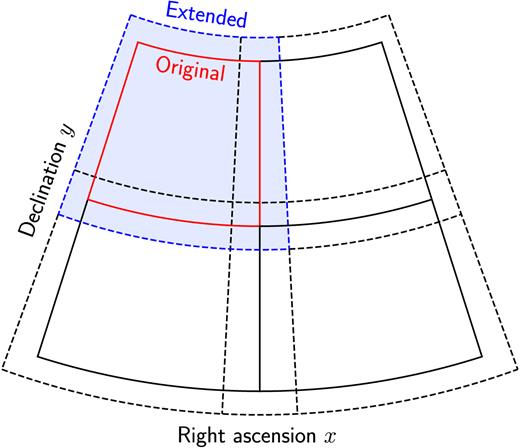
Illustration of the tiled geometry in the gnomonic projection. Solid boxes: Original tiles. Dashed boxes: Temporarily extended tiles. For a better distinction, the first tile is coloured.

Open in new tab Download slide

The computations are performed on regular mesh grids with default resolutions of 0.25 arcsec/px. Celestial coordinates are locally mapped to the tangent plane by a gnomonic projection (e.g. Calabretta & Greisen 2002). A vector-valued grid is defined for the weighted effective luminosity maps |$\smash{\tilde{K}^{(l)}_{\mathrm{gal}} L^{(l)}}$| and |$\smash{\tilde{K}^{(l)}_{\mathrm{clus}} L^{(l)}}$|⁠, from which scalar-valued grids are derived via line-of-sight projection and convolved with the kernels G and C according to equation (37). The confluent hypergeometric function ₁F₁ is evaluated using common approximation schemes (e.g. Muller 2001; Pearson, Olver & Porter 2017).

For the numerical solution of the convolutions, we use discrete Fast Fourier methods (Cooley & Tukey 1965) and exploit the discrete convolution theorem (Cochran et al. 1967), which allows us to substitute the Fourier transform of a convolution by a product of Fourier transforms. For the subsequent differentiation of the lensing potential, we apply suitable definitions of forward, backward, and central finite differences. The angular finite differences are locally approximated by Cartesian finite differences.

5.2 Critical curve recognition

EasyCritics computes the Jacobian eigenvalues and the determinant based on equation (17) by finite differentiation of the lensing potential. It derives a binary map of regions with a negative determinant by applying a Heaviside step function:

\begin{eqnarray*} B(\boldsymbol{\theta }) = \Theta (-\det \mathbf {J}). \end{eqnarray*}

(38)

It then retrieves the contours of all connected components |$\lbrace \boldsymbol{\theta }: B(\boldsymbol{\theta }) = 1 \rbrace$| via border following (Suzuki & Abe 1985). As an option, radial critical curves can be removed or grouped together with the tangential lines.

For each contour, the centroid |$(\bar{\theta }_1, \bar{\theta }_2)$|⁠, the orientation ϕ, and the principal axis lengths a, b are determined by an analysis of second-order image moments (Hu 1962; Stobie 1986), as defined in Appendix C. The geometrical parameters determined in this way enable a selection of targets for subsequent searches based on position and size. In order to avoid pixel artefacts due to the central cusp in our power-law description of the galaxy-scale subhaloes, EasyCritics discards all detections with an effective Einstein radius below a certain threshold, defined as the equivalent circle radius, |$\theta _{\mathrm{E,eff}} \equiv \sqrt{A/{\pi} }$| (Puchwein & Hilbert 2009; Zitrin et al. 2011a). In this study, we apply the empirically motivated value θ_{E, eff} ∼ 1.5 arcsec.

The different steps of the recognition algorithm are illustrated for an example cluster-scale detection in Fig. 3. For each set of critical pixels, the pixel coordinates are stored in critical curve catalogues together with the geometrical parameters |$\bar{\theta }_1$|⁠, |$\bar{\theta }_2$|⁠, ϕ, a, b and the effective Einstein radius θ_{E, eff}.

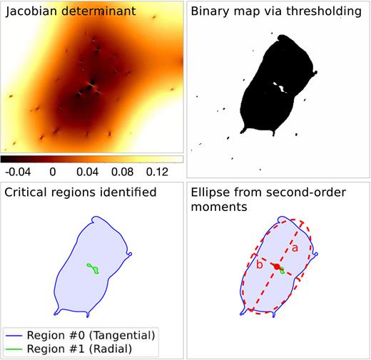
$Illustration of the critical curve recognition for a region centred on a cluster-scale detection. Top left: Jacobian determinant. Top right: Binary map $B(\boldsymbol{\theta })$ from thresholding. Bottom left: Detected regions and their contours, displayed as filled polygons. Bottom right: Ellipse from the moment calculation for the tangential critical curve.$

Figure 3.

Illustration of the critical curve recognition for a region centred on a cluster-scale detection. Top left: Jacobian determinant. Top right: Binary map |$B(\boldsymbol{\theta })$| from thresholding. Bottom left: Detected regions and their contours, displayed as filled polygons. Bottom right: Ellipse from the moment calculation for the tangential critical curve.

Open in new tab Download slide

5.3 Parameter calibration

The free model parameters |$\smash{P = \lbrace q, \sigma , \tilde{K}_{\mathrm{gal}}, \tilde{K}_{\mathrm{clus}}, n_\mathrm{ c} \rbrace }$| are calibrated by fitting critical curves to the arcs of previously known lenses. During the calibration, we use a physically equivalent, but more convenient representation of the model parameters, |$\smash{P^{\prime } = \lbrace q, \sigma , K, \mu _{\mathrm{clus}}, n_\mathrm{ c}\rbrace }$|⁠, by introducing the two independent quantities:

\begin{eqnarray*} K &\equiv& K_{\mathrm{gal}} + K_{\mathrm{clus}}, \nonumber \\ \mu _{\mathrm{clus}} &\equiv& \frac{K_{\mathrm{clus}}}{K_{\mathrm{gal}} + K_{\mathrm{clus}}}. \end{eqnarray*}

(39)

This allows us to consider the relative amplitudes of the two mass components independently and to better cope with inherent lensing degeneracies between q, |$\smash{K_{\mathrm{gal}}}$|⁠, and |$\smash{K_{\mathrm{clus}}}$|⁠.

Since arcs and multiple images are expected to form in the vicinity of critical curves, we use their locations and geometry to constrain the approximate positions of the critical curves (e.g. Narayan & Bartelmann 1996; Meneghetti et al. 2007a). In a least-squares approach, we derive the free parameters P by fitting the squared tangential⁵ Jacobian eigenvalues |$\lambda (P, \boldsymbol{\theta }_i)$| within a set of N ‘arc pixels’ Θ_crit that are assigned to be part of the critical curve:

\begin{eqnarray*} \chi ^2(P) = \frac{1}{N} \sum _{ \boldsymbol{\theta }_i \in \Theta _{\mathrm{crit}}} \vert \lambda (P, \boldsymbol{\theta }_i) \vert ^2. \end{eqnarray*}

(40)

This expresses the expectation that the eigenvalues vanish along the critical curve traced by the reference pixels, given a set of parameters P. The eigenvalue-based criterion provides a local and robust least-squares estimate that generalizes the determinant-based objective function used by Cacciato et al. (2006). The specific positions and number of the pixels Θ_crit are defined by the user in order to keep the method flexible. Depending on the specific data set under consideration, the Θ_crit could represent pixels containing giant arcs, the positions of multiple images, or model-independent constraints from lensed images (e.g. Merten et al. 2009; Wagner 2017). In this study we use pixels randomly sampled over giant arcs, as explained in Section 6. These trace the critical curves to good approximation within the uncertainties of the LTM approach (Meneghetti et al. 2007a).

For an efficient minimization procedure, we have developed a parallelized generalization of the Metropolis–Hastings algorithm (Metropolis et al. 1953; Hastings 1970), which is able to perform up to 10 |$\smash{\chi ^2}$|-evaluations per second by combining Markov Chain Monte Carlo (MCMC) sampling with an innovative use of adaptive grid methods. In particular, the randomly drawn variates for q and σ characterizing the shapes of the kernels G and C are binned on a regular grid (cf. Fig. 4) in order to reuse intermediate results between the sampling steps, while retaining the Gaussian distribution of the priors. The parameter space is explored by multiple threads in parallel, which update the mean values of their prior distributions periodically according to the global χ² minimum. Around this minimum, the grid can be iteratively refined to achieve a higher accuracy and precision. With this scheme, the runtime is reduced by orders of magnitude when compared with a standard MCMC approach (see Section 5.4 for runtime measurements). The MCMC approach is optimally suited for our purpose, because it enables to deal with non-convex objective functions as well. Moreover, it requires no additional parameters to tune the algorithm.

Figure 4.

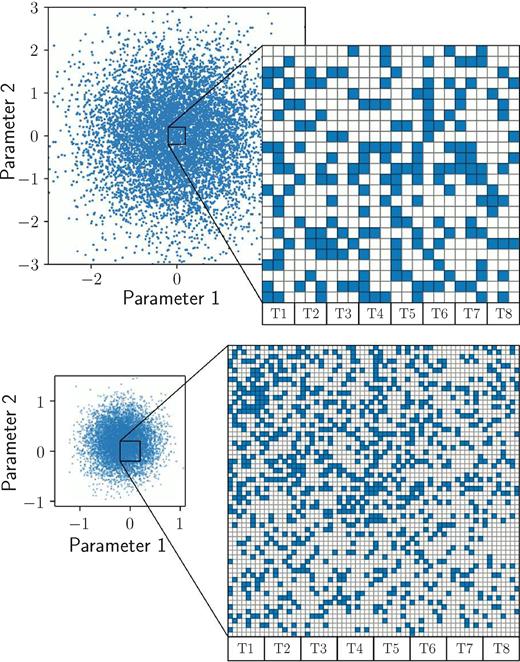
Illustration of the adaptive grid-based MCMC method for a two-dimensional parameter space: Gaussian random variates are sampled on a fine regular grid (top), which is iteratively refined in size and resolution (bottom) according to the previous optimum. The computation is performed column-wise, distributed on a given number of threads, in this example eight (T1–T8).

Open in new tab Download slide

In contrast to the other parameters, the critical number density n_c is defined based on the number of LRGs used. In the current implementation, we keep n_c constant at an empirically determined value of n_c ≈ 65/(15 arcmin × 15 arcmin) per sheet.

Currently, the calibration can be performed on individual known lenses to obtain independent sets of parameters, which then need to be combined appropriately. In an upcoming implementation, we are going to introduce a multilens calibration, in which all parameters are fitted to a larger set of known lenses simultaneously, optimizing the detection rate and the number of predictions to obtain the most efficient set of parameters, which is able to provide the best description for a broad range of lensing mass distributions.

5.4 Performance

Due to the large area that needs to be explored with the calibrated parameter sets, as well as the large number of MCMC sampling steps to be evaluated during the calibration itself, an optimization of the code design for cost-efficiency, i.e. for a low consumption of time and memory, is of critical importance. For the cost-efficiency to scale well with both the number of parallel processes and the problem size, we aim at a maximal parallel portion⁶ (Amdahl 1967) and weak scalability. In our implementation, we apply these criteria by using discrete fast Fourier methods for the convolutions and by parallelizing the computation of lensing quantities using the OpenMP⁷ interface. As an option, specific instructions can be accelerated on a CUDA⁸-capable GPU, if available.

In Appendix D, we present runtime measurements for the calibration and application phases on a recent 64-bit consumer PC⁹ when EasyCritics is applied to a realistic scenario and using different numbers of CPU cores. We compare and discuss these results in the context of strong and weak scalability. The typical runtime for a single calibration step remains below a second even in single-thread mode, demonstrating the advantages of the adaptive, grid-based MCMC method. The application to a |$\smash{1 \, \mathrm{deg^2}}$| region takes less than a minute on a commercial CPU. In comparison with crowdsourced visual inspection, these time-scales represent a significant improvement. The visual inspection of a |$\smash{154 \, \mathrm{deg^2}}$| region by 37 000 volunteers can require up to eight months (Marshall et al. 2016). For upcoming |$\smash{\gtrsim 10^4 \, \mathrm{deg^2}}$| surveys, such an analysis would require the same number of people to inspect the images for half a lifetime, highlighting the high costs and low efficiency of visual inspection. In contrast, EasyCritics is able to analyse |$\smash{10^4 \, \mathrm{deg^2}}$| on time-scales of days or weeks¹⁰ on a consumer PC, once calibrated.

6 APPLICATION EXAMPLES

As a first test to investigate and demonstrate the concepts discussed in this work, we apply EasyCritics to the CFHTLenS data set (Heymans et al. 2012; Erben et al. 2013; Miller et al. 2013). CFHTLenS is a wide-field photometric survey that covers |$\smash{154 \, \mathrm{deg}^2}$| and provides optical images in the five broad-band filters u*, g′, r′, i′, |$z$|′. With a depth of m_lim = 25.5 in the i′-band, sub-arcsecond seeing conditions and accurate photometric redshifts, the CFHTLenS imaging data and object catalogues are well suited for gravitational lensing studies (Hildebrandt et al. 2012; Erben et al. 2013).

For the use with EasyCritics, we filter the object catalogues for early-type galaxies by removing all stellar sources and objects with a spectral type¹¹T_B > 1.7 according to the classification by Coleman, Wu & Weedman (1980). We apply a k-correction to the fluxes and magnitudes of the galaxies using the template spectra described by Capak (2004) and the final transmittance curves of the MegaCam filters.¹² However, the k-correction does not have a strong impact on the results because it is to a large part degenerate with the free model parameter K and, over small redshift ranges, could be absorbed into the calibration. For the computation of cosmological distances, we use a ΛCDM model with Planck 2015 parameter values (Planck Collaboration XIII 2016).

We apply EasyCritics to a subset of four individual lenses, selecting well-studied objects that cover small and large structures. We start by calibrating the parameters on two known lenses, a small group (‘A’) and a rich cluster (‘B’). This yields the two independent parameter sets P_A and P_B. Applying both sets one after each other, we then test whether EasyCritics is able to predict critical curves around two further known lenses ‘C’ and ‘D’. As a consistency check, we perform also a reverse test by calibrating the model parameters against the lenses C and D and applying them to the lenses A and B. Moreover, we apply EasyCritics to a |$\smash{1 \, \mathrm{deg}^2}$| field in which no group- and cluster-scale lens candidates have been reported yet. The four calibrations are summarized in Section 6.2 and the resulting predictions are presented and discussed in Section 6.3. In Section 6.4, we estimate how the results are affected by uncertainties with regard to the lens and source redshifts .

Note that a full assessment of the detection efficiency, using the entire survey area and simulations, is beyond the scope of this work and will be presented in our upcoming papers (Carrasco et al. 2018; Stapelberg et al. , in preparation).

6.1 Selection of known lenses

The lenses A–D are representative for the group- and cluster-scale lenses reported in CFHTLens. Three of the lenses (A, B, C) are extracted from the CFHTLS Strong Lensing Legacy Survey (SL2S; Cabanac et al. 2007; More et al. 2012) and one (D) from the newly reported lenses by SpaceWarps (SW; Marshall et al. 2016; More et al. 2016) that has so far been missed by automated methods. The four examples are chosen to ‘challenge’ EasyCritics by including lenses with very different properties: (1) The lenses are located in areas with different depths and environmental properties; (2) The lenses represent different regimes in Einstein radii, masses, and redshifts; (3) The lenses have different numbers of arcs, ranging from 1 to 3 arcs/images. Below, we briefly introduce all four objects and describe their main characteristics:

Lens A: The first object is a compact group of galaxies, SL2S J021408-053532 or SA22,¹³ located at |$z$|_phot = 0.48 ± 0.02 (More et al. 2012). It shows a fold configuration of two arcs (A1, cf. Fig. 5) at |$z$|_spec = 1.628 ± 0.001 and a possible third feature (A2, cf. Fig. 5) observed at |$z$|_spec = 1.017 ± 0.001 (Verdugo et al. 2011, 2016). The apparent Einstein radius amounts to θ_E ∼ 7.1 arcsec. A combined dynamical and parametric lensing mass reconstruction carried out by Verdugo et al. (2016) suggests that the centres and orientations of the main dark matter halo, the intracluster gas halo, and the luminosity contours are in good agreement if fitting a NFW profile for the main group halo and pseudo-isothermal ellipses to the central galaxy haloes.
Lens B: The second object is the galaxy cluster SL2S J141447 + 544703 or SA100 (Cabanac et al. 2007) at |$z$|_phot = 0.63 ± 0.02 (More et al. 2012), which is known to be a Sunyaev-Zel’dovich bright cluster (PSZ1 G099.84 + 58.45; Planck Collaboration XXIX 2014; Gruen et al. 2014). It shows a tangential giant arc (B1, cf. Fig. 5), whose redshift, however, has not yet been measured spectroscopically. With an apparent Einstein radius of θ_E ∼ 14.7 arcsec, the cluster belongs to the largest strong lenses imaged by CFHTLenS.
Lens C: The third object is the galaxy group SL2S J08544-0121 or SA66 at |$z$|_spec = 0.351 (Limousin et al. 2009), which stands out by a bimodal light distribution with luminosity peaks separated by |$\smash{\gtrsim 50\rm{\,arcsec}}$|⁠. One of these peaks is associated with a bright, double-cored galaxy, near which a typical cusp configuration at |$z$|_spec = 1.2680 ± 0.0003 (Limousin et al. 2010) is observed. The latter shows three images merging into a giant arc and a bright counter image (cf. Fig. 6). The lens has an Einstein radius of 4.8 arcsec and appears to be dominated by a single massive galaxy, which makes this candidate an ideal application target for testing the limits of EasyCritics towards smaller scales.
Lens D: The fourth object is the small cluster J220257 + 023432 or SW7 at redshift¹⁴|$z$|_phot ∼ 0.51, which shows two very promising, although partially faint and overblended giant arc candidates (cf. Fig. 6) at a radius θ_E ∼ 6.8 arcsec. These have been newly reported as secure detections by SW (More et al. 2016) after they were missed by various automated algorithms applied within the region (e.g. More et al. 2012). The strongly lensing system is an interesting case to test the potential of the arc-free search approach underlying EasyCritics, since a successful detection and identification of this object as a strong lens would be the first achieved with a fully automated method.

Figure 5.

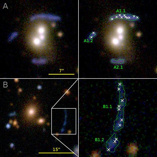
Illustration of the calibration for lenses A and B. The figure shows CFHTLenS i′r′g′-composite images with the arc regions (green contours) and the random χ²-minimization pixels Θ_crit (white crosses) used in Section 6.2.

Open in new tab Download slide

Figure 6.

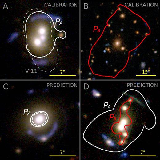
Calibrated and predicted tangential critical curves for the first test scenario, shown on CFHTLenS i′r′g′-composite images. Top row: Calibrations P_A and P_B on the two lenses A and B (solid lines) and literature comparison showing the model of Verdugo et al. (2011, V’11). Bottom row: Predictions for lenses C and D using P_A and P_B and assuming |$z$|_s = 2 (solid lines) and for lens C the known value |$z$|_s = 1.268 (dashed line).

Open in new tab Download slide

6.2 Calibrations

In the following, we describe the four independent calibrations on lenses A–D and discuss their results. For each lens, the model parameters are estimated via the MCMC-based critical curve fitting method described in Section 5.3. In case that there is more than one configuration of known arcs, we select that covering the largest area. Where available, we use spectroscopic information on the source redshift. For the initial parameter values and ranges, we apply empirically motivated values, which are specified in Table 2. The MCMC sampler is initialized with a Gaussian random distribution that has a width σ_r = 0.4Δ_r, with Δ_r denoting the interval considered for the respective parameter.

Table 2.

Open in new tab

Initial parameter values and ranges considered for the calibration, where K is given in arbitrary units.

	q	K	μ_clus	σ (arcsec)
Lower limit:	1.10	\|$\hphantom{10}5$\|	0.70	\|$\hphantom{1}3$\|
Initial value:	1.25	\|$\hphantom{1}47$\|	0.85	10
Upper limit:	1.40	100	0.95	20

	q	K	μ_clus	σ (arcsec)
Lower limit:	1.10	\|$\hphantom{10}5$\|	0.70	\|$\hphantom{1}3$\|
Initial value:	1.25	\|$\hphantom{1}47$\|	0.85	10
Upper limit:	1.40	100	0.95	20

Table 2.

Open in new tab

Initial parameter values and ranges considered for the calibration, where K is given in arbitrary units.

	q	K	μ_clus	σ (arcsec)
Lower limit:	1.10	\|$\hphantom{10}5$\|	0.70	\|$\hphantom{1}3$\|
Initial value:	1.25	\|$\hphantom{1}47$\|	0.85	10
Upper limit:	1.40	100	0.95	20

	q	K	μ_clus	σ (arcsec)
Lower limit:	1.10	\|$\hphantom{10}5$\|	0.70	\|$\hphantom{1}3$\|
Initial value:	1.25	\|$\hphantom{1}47$\|	0.85	10
Upper limit:	1.40	100	0.95	20

The positions of the pixels Θ_crit to be used for the eigenvalue minimization are sampled randomly over the areas covered by the arcs, as illustrated in Fig. 5. These areas are defined by a visual selection of suitable g′-band contours. As discussed in Section 5.3, the true path of the critical curve is in principle unknown, but it can be approximated to good accuracy by the positions of the arcs for an estimation of the LTM model parameters. The uncertainty Δχ² is estimated based on the largest difference in the squared Jacobian eigenvalues within the selection area. The final outcome of the calibration is given by the set sitting in the global minimum within Δχ². The uncertainties of the individual parameters are estimated by computing the second moments among all MCMC samples within a separation of Δχ² from the optimum. These are used to compare different calibrations in order to test for compatibility between data sets and to probe the influence of other uncertainties, as it will be addressed in Section 6.4.

We present the four results P_A to P_D together with their 1σ uncertainties due to Δχ² in Table 3 and show the associated best-fitting critical curves in Figs 6 and 7. The fits converged within |$\smash{N \lesssim \mathcal {O}(10^5)}$| sampling steps, resulting in final least-square deviations between |$\smash{\chi ^2 \sim \mathcal {O}(10^{-3})}$| and |$\smash{\chi ^2 \sim \mathcal {O}(10^{-2}})$|⁠. The calibrated critical curves qualitatively match our expectation. For instance, the result for lens A resembles the lens modelling reconstruction of Verdugo et al. (2011) well. In Fig. 6, we compare the critical curve obtained with our approach (solid line) and the result of Verdugo et al. (dashed line). A slight deviation can be noted in the bottom image region, but this is well explained by a slight misalignment between the smoothed r′-band luminosity isocontours and the total mass. For lens D, the shape of the predicted critical curve might have been affected slightly too much by local galaxies in the proximity of the northern giant arc candidate. However, its location and size match the arcs well.

Figure 7.

Calibrated and predicted tangential critical curves for the second test scenario. Top row: Calibrations P_C and P_D on the lenses C and D. Bottom row: Tangential critical curves predicted for lenses A and C by P_C and P_D, assuming |$z$|_s = 2 where the source redshift is not known.

Open in new tab Download slide

Table 3.

Open in new tab

Calibration results for all four lenses A–D. The parameter K is given in arbitrary units.

Lens	q	K	μ_clus	σ (arcsec)
A	1.24 ± 0.02	37 ± 7	0.84 ± 0.01	10 ± 1
B	1.22 ± 0.02	35 ± 7	0.93 ± 0.01	18 ± 1
C	1.28 ± 0.01	68 ± 6	0.81 ± 0.01	5 ± 1
D	1.26 ± 0.02	40 ± 7	0.81 ± 0.02	10 ± 1

Lens	q	K	μ_clus	σ (arcsec)
A	1.24 ± 0.02	37 ± 7	0.84 ± 0.01	10 ± 1
B	1.22 ± 0.02	35 ± 7	0.93 ± 0.01	18 ± 1
C	1.28 ± 0.01	68 ± 6	0.81 ± 0.01	5 ± 1
D	1.26 ± 0.02	40 ± 7	0.81 ± 0.02	10 ± 1

Table 3.

Open in new tab

Calibration results for all four lenses A–D. The parameter K is given in arbitrary units.

Lens	q	K	μ_clus	σ (arcsec)
A	1.24 ± 0.02	37 ± 7	0.84 ± 0.01	10 ± 1
B	1.22 ± 0.02	35 ± 7	0.93 ± 0.01	18 ± 1
C	1.28 ± 0.01	68 ± 6	0.81 ± 0.01	5 ± 1
D	1.26 ± 0.02	40 ± 7	0.81 ± 0.02	10 ± 1

Lens	q	K	μ_clus	σ (arcsec)
A	1.24 ± 0.02	37 ± 7	0.84 ± 0.01	10 ± 1
B	1.22 ± 0.02	35 ± 7	0.93 ± 0.01	18 ± 1
C	1.28 ± 0.01	68 ± 6	0.81 ± 0.01	5 ± 1
D	1.26 ± 0.02	40 ± 7	0.81 ± 0.02	10 ± 1

Table 4.

Open in new tab

Summary of quantitative results from Sections 6.2 and 6.3.

Lens	Right ascension	Declination δ	Lens	Detected?	Arc radius	Calibrated eff. Einstein	Predicted eff. Einstein
	α (J2000) (deg)	(J2000) (deg)	redshift \|$z$\|_l	(No. of curves)	θ_E (arcsec)	radius θ_{E, eff} (arcsec)	radii θ_{E, eff} (arcsec)
A	33.5336	−5.5922	0.48	Yes (2)	7.1	5	P_C: 15;	P_D: 4
B	213.6965	+54.7842	0.63	Yes (2)	14.7	21	P_C: 29;	P_D: 12
C	133.6940	−1.3603	0.351	Yes (1)	4.8	5	P_A: 2	–
D	330.7372	+2.5760	0.51	Yes (2)	6.8	6	P_A: 8;	P_B: 3
\|$1 \, \mathrm{deg}^2$\| field	215.3273	+55.2480	0.3...0.4	–	–	–	P_C: 3	–

Lens	Right ascension	Declination δ	Lens	Detected?	Arc radius	Calibrated eff. Einstein	Predicted eff. Einstein
	α (J2000) (deg)	(J2000) (deg)	redshift \|$z$\|_l	(No. of curves)	θ_E (arcsec)	radius θ_{E, eff} (arcsec)	radii θ_{E, eff} (arcsec)
A	33.5336	−5.5922	0.48	Yes (2)	7.1	5	P_C: 15;	P_D: 4
B	213.6965	+54.7842	0.63	Yes (2)	14.7	21	P_C: 29;	P_D: 12
C	133.6940	−1.3603	0.351	Yes (1)	4.8	5	P_A: 2	–
D	330.7372	+2.5760	0.51	Yes (2)	6.8	6	P_A: 8;	P_B: 3
\|$1 \, \mathrm{deg}^2$\| field	215.3273	+55.2480	0.3...0.4	–	–	–	P_C: 3	–

Table 4.

Open in new tab

Summary of quantitative results from Sections 6.2 and 6.3.

Lens	Right ascension	Declination δ	Lens	Detected?	Arc radius	Calibrated eff. Einstein	Predicted eff. Einstein
	α (J2000) (deg)	(J2000) (deg)	redshift \|$z$\|_l	(No. of curves)	θ_E (arcsec)	radius θ_{E, eff} (arcsec)	radii θ_{E, eff} (arcsec)
A	33.5336	−5.5922	0.48	Yes (2)	7.1	5	P_C: 15;	P_D: 4
B	213.6965	+54.7842	0.63	Yes (2)	14.7	21	P_C: 29;	P_D: 12
C	133.6940	−1.3603	0.351	Yes (1)	4.8	5	P_A: 2	–
D	330.7372	+2.5760	0.51	Yes (2)	6.8	6	P_A: 8;	P_B: 3
\|$1 \, \mathrm{deg}^2$\| field	215.3273	+55.2480	0.3...0.4	–	–	–	P_C: 3	–

Lens	Right ascension	Declination δ	Lens	Detected?	Arc radius	Calibrated eff. Einstein	Predicted eff. Einstein
	α (J2000) (deg)	(J2000) (deg)	redshift \|$z$\|_l	(No. of curves)	θ_E (arcsec)	radius θ_{E, eff} (arcsec)	radii θ_{E, eff} (arcsec)
A	33.5336	−5.5922	0.48	Yes (2)	7.1	5	P_C: 15;	P_D: 4
B	213.6965	+54.7842	0.63	Yes (2)	14.7	21	P_C: 29;	P_D: 12
C	133.6940	−1.3603	0.351	Yes (1)	4.8	5	P_A: 2	–
D	330.7372	+2.5760	0.51	Yes (2)	6.8	6	P_A: 8;	P_B: 3
\|$1 \, \mathrm{deg}^2$\| field	215.3273	+55.2480	0.3...0.4	–	–	–	P_C: 3	–

A quantitative comparison of the best-fitting parameter values for the lenses P_A to P_D listed in Table 3 shows that the scatter in q and K between the lenses within the estimated uncertainties is low despite the large difference in the redshift and Einstein radii of the lenses. As expected, the largest differences between all four parameter sets are found between lenses B and C. Despite a possible impact of the low number of satellites on the M/L estimate in the case of lens C (Lu, Yang & Shen 2015), the different values obtained for K are consistent with the expected scatter in the M/L ratios of groups and clusters (e.g. Lin et al. 2004; Tinker et al. 2005; Bahcall & Kulier 2014; Lu et al. 2015; Viola et al. 2015; Mulroy et al. 2017).

6.3 Identification of known lenses

For each of the four lenses, we apply EasyCritics to a 5 arcmin × 5 arcmin (extended: 15 arcmin × 15 arcmin) region around the cD galaxies. The precise centre of the region is not relevant because in a general application, the algorithm is run over the entire data set. For a positive detection, we require that at least one of the parameter sets produces a critical curve with a centroid separated by less than 40 arcsec from the expected lens centre.¹⁵ The choice of this maximum distance accounts for intrinsic offsets between the dark and luminous matter components. In addition, we investigate the agreement of the predicted critical curves with those obtained from the calibrations, which represent the best fit of our LTM model. This allows us to study the impact of the intrinsic variation of lens parameters on the model predictions.

In general, the variation of parameters from lens to lens is expected to yield slight deviations of the predicted Einstein radii from the true ones. These, however, are well within the aims of lens detection. In fact, the goal is not a precise reconstruction of the mass, which can be achieved only via a subsequent fit, but to find the regions in which strong lensing features are produced. Thus, the sensitivity of the predicted critical curves to variations in the model parameters should become relevant only to the extent to which it may affect the detection rate or the area for follow-up inspection. An extensive analysis of the detection efficiency of EasyCritics for different settings will be the subject of upcoming papers (Carrasco et al. 2018). Here, we focus on the individual performance of the parameter sets P_A to P_D.

The tests yield positive outcomes for all four lenses. Each lens is identified by each parameter set, except for lens C, for which a critical curve is produced only by the group-scale set P_A. This, however, is not surprising given the very low richness of lens C, for which P_A may provide a better description than P_B. A more remarkable result is the successful identification of the SW lens candidate D, as it had been missed by several automated methods before (More et al. 2012). This demonstrates the importance and benefits of using foreground search criteria complementary to arc data, thus avoids problems due to low signal-to-noise ratios, complex morphologies, or overblending.

A comparison of all four predicted critical curves is shown in Figs 6 and 7. Not surprisingly, the parameters obtained from small/large lenses perform best when applied to the other small/large lenses. At the same time, the smallest scale calibrations P_C and P_D show an overall better performance than the cluster-scale calibration P_B by predicting critical curves with either large or compatible Einstein radii for all mass regimes, while P_B strongly underestimates the surface density on group scales. This is because a small Gaussian width σ (resulting from the calibration on a small lens) applied to large lenses is still going to result in cluster-scale haloes concentrated enough to produce critical curves close to the Einstein radii, which is no longer the case when applying a large σ to small lenses. In this case, the predicted cluster-scale component is spread over a large area producing an excessive dilution that can prevent the appearance of critical regions. This effect is illustrated in Fig. 8 for the example of lens B, where it gets further enhanced by the fact that multiple haloes are superposed. In contrast, the remaining parameters q, K, μ_clus have a much smaller influence on the model. This would allow to fix fiducial values for these parameters and to perform an optimization on the parameter σ in order to reduce the degrees of freedom of the model, at least for the sample of lenses studied here.

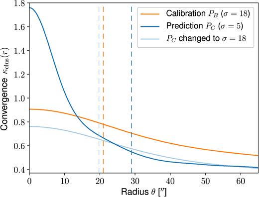
$Comparison of the convergence profile $\bar{\kappa }_{\mathrm{clus}}(r)$ for the smooth cluster-scale component of lens B, illustrating the behaviour of different sizes σ for the Gaussian smoothing kernel. The curves show the profiles computed for PB, PC and when using PC with the value σ from PB. The dashed lines mark the predicted effective Einstein radii θE, eff.$

Figure 8.

Comparison of the convergence profile |$\bar{\kappa }_{\mathrm{clus}}(r)$| for the smooth cluster-scale component of lens B, illustrating the behaviour of different sizes σ for the Gaussian smoothing kernel. The curves show the profiles computed for P_B, P_C and when using P_C with the value σ from P_B. The dashed lines mark the predicted effective Einstein radii θ_{E, eff}.

Open in new tab Download slide

In the remaining part of our tests, we apply EasyCritics to a |$\smash{1 \, \mathrm{deg}^2}$| field for which no group- or cluster-scale strong lens candidates have been reported by the SL2S (Cabanac et al. 2007; More et al. 2012), by SW¹⁶ (More et al. 2016), or in NED¹⁷ (Helou et al. 1995). In contrast to the previous examples, we display a case for a low-density region in which we expect to find either new or no critical regions. In this field, EasyCritics produces only a single critical curve on group or cluster scales with θ_{E, eff} ≈ 3 arcsec, found by the set P_C and centred around what appears to be an elongated small cluster (‘E’). The latter can be estimated to be at |$z$| ∼ 0.3…0.4 based on the photometric redshifts of the elliptical galaxies in the region. In addition, very few critical curves are produced around single isolated field galaxies, all having Einstein radii θ_{E, eff} < 2.75 arcsec. These features are mostly artificial detections due to the central cusp in our description of galaxies, which can give rise to few pixels with supercritical surface densities. They can be avoided easily by increasing the critical curve size threshold or by a slight modification of the parameter values. For instance, in configuration P_B, only one of these objects is created. A map of the convergence for the entire region and a zoom-in on the central region of candidate E is presented in Fig. 9.

An overview of the calibration and detection results is presented in Table 4.

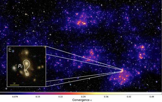
$Cluster-scale convergence predicted with parameter set PC for the candidate-free $1 \, \mathrm{deg}^2$ region, superimposed on a CFHTLenS i′r′g′-composite image. The box on the left shows a zoom-in on the critical curve of the only group-scale critical curve detection.$

Figure 9.

Cluster-scale convergence predicted with parameter set P_C for the candidate-free |$1 \, \mathrm{deg}^2$| region, superimposed on a CFHTLenS i′r′g′-composite image. The box on the left shows a zoom-in on the critical curve of the only group-scale critical curve detection.

Open in new tab Download slide

6.4 Impact of redshift uncertainties

Apart from the intrinsic variation in the best-fitting parameters, some impacts on the models may arise due to the photometric redshift measurement uncertainty, Δ|$z$|_phot, and the intrinsic scatter of the source redshifts, Δ|$z$|_s. Both could mildly affect the detection statistics by altering the calibration and the predicted sizes of critical curves. In order to estimate at least the order of magnitude of these effects, we study how the critical curves are affected by small displacements in the lens and source redshifts and compare this to the previously discussed sources of uncertainty. The results obtained in this way are very similar for all four lenses and in the following discussed in detail for the example of the cluster-scale lens B, which is farthest away in redshift and thus may be affected the most by the photometric uncertainties.

We first investigate the sensitivity of predicted critical curve sizes to the average photometric measurement uncertainty Δ|$z$|_phot = 0.04(1 + |$z$|⁠) of the CFHTLenS data (cf. Hildebrandt et al. 2012). We displace all redshift bins by Gaussian random variates with a mean μ_r = |$z$|^(k) and a standard deviation σ_r = Δ|$z$|_phot, while keeping the parameters fixed at the calibration set P_B. The procedure is performed 200 times, yielding the critical curves shown in the left-hand panel of Fig. 10. The mean Einstein radius is θ_{E, eff} = 21 arcsec with a standard deviation of 2.6 arcsec. The results confirm our expectation that the photometric measurement uncertainties influence the sizes of the critical curves mildly, although leaving the overall outcome unchanged. We repeat the calibration for the random displacements that yielded critical curve sizes closest to the 1σ neighbourhood around the mean to estimate the impact of Δ|$z$|_phot on the parameter values. The results are shown in Table 5.

Figure 10.

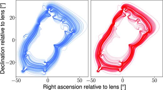
Impact of the mean photo-|$z$| uncertainties (left/blue) and the source redshift uncertainties (right/red). Shown are in both cases the tangential critical curves of lens B produced with P_B for different random displacements of the redshifts, as described in Section 6.4. For a clearer presentation, we only show every second of the 200 lines.

Open in new tab Download slide

Table 5.

Open in new tab

Comparison of absolute uncertainties in the calibrated parameter values due to (1) redshift misestimations, (2) the degeneracy between optimization points, and (3) the intrinsic deviation of P_B from P_A.

Parameter	Dev. due	Dev. due	Dev. due	Dev.
	to Δ\|$z$\|_phot	to Δ\|$z$\|_s	to Δχ²	from P_A
q	0.05	0.01	0.02	0.02
K	16	4.5	7	2
μ_clus	0.04	0.01	0.01	0.09
σ	2	2	1	8

Parameter	Dev. due	Dev. due	Dev. due	Dev.
	to Δ\|$z$\|_phot	to Δ\|$z$\|_s	to Δχ²	from P_A
q	0.05	0.01	0.02	0.02
K	16	4.5	7	2
μ_clus	0.04	0.01	0.01	0.09
σ	2	2	1	8

Table 5.

Open in new tab

Comparison of absolute uncertainties in the calibrated parameter values due to (1) redshift misestimations, (2) the degeneracy between optimization points, and (3) the intrinsic deviation of P_B from P_A.

Parameter	Dev. due	Dev. due	Dev. due	Dev.
	to Δ\|$z$\|_phot	to Δ\|$z$\|_s	to Δχ²	from P_A
q	0.05	0.01	0.02	0.02
K	16	4.5	7	2
μ_clus	0.04	0.01	0.01	0.09
σ	2	2	1	8

Parameter	Dev. due	Dev. due	Dev. due	Dev.
	to Δ\|$z$\|_phot	to Δ\|$z$\|_s	to Δχ²	from P_A
q	0.05	0.01	0.02	0.02
K	16	4.5	7	2
μ_clus	0.04	0.01	0.01	0.09
σ	2	2	1	8

In a second test, we investigate the change in the calibrated and predicted critical curves when the source redshift differs from our default expectation value |$z$|_s = 2. This does not represent a test of the lens model itself, but of its dependence on the source redshift only. We first study the change in predicted critical curves by re-applying the parameter values P_B calibrated under the assumption |$z$|_s = 2 to lens B, using 200 random redshift displacements within the empirically motivated range of bright giant arcs, |$z$|_s = 2.0 ± 0.1 (Bayliss 2012). The critical curves predicted for these different source redshifts are visualized in the right-hand panel of Fig. 10. The effective Einstein radii are distributed with a mean of θ_{E, eff} = 21 arcsec and a standard deviation of 2 arcsec. As before, we also study the impact on the calibration by repeating the calibration for the various source redshifts, which yields the maximum differences Δ|$z$|_s in the final best-fitting parameters P_B listed in Table 5.

The tests show that the detection of the critical curve itself is stable with respect to the redshift uncertainties Δ|$z$|_phot and Δ|$z$|_s, although the critical curve may vary in size. In extreme cases, this might affect the completeness of predictions due to underestimating the size of critical curves.

7 SUMMARY AND CONCLUSIONS

We have developed an algorithm to detect group- and cluster-scale strong lenses in wide-field surveys, based on the distribution of fluxes from LRGs as a tracer for dense structures. EasyCritics models these structures in a blind and automated way to identify the most likely strongly lensing groups and clusters of galaxies. This promises to avoid a large number of spurious detections and to decrease the required amount of post-processing, as it significantly reduces and restricts the area that needs to be validated or inspected by a follow-up study. The main advantage of EasyCritics is that it enables a simple, physically motivated selection criterion based on few model assumptions and without relying on the identification of arcs. In addition, EasyCritics provides a first characterization of the properties of lens candidates, such as their positions, surface densities, Einstein radii, and orientations of the critical curves.

In this work, we presented a modified and numerically improved version of the LTM modelling approach, based on the brightest early-type galaxies distributed along the line of sight. In particular, EasyCritics blindly models the lensing distortion produced within the entire line of sight (not only pre-selected, isolated structures) and derives lensing quantities from a potential instead of working with the deflection angle. In combination with the use of parallelization and fast Fourier and matrix calculation routines, this allows us to obtain a substantial speed-up in the identification and modelling of strongly lensing structures. The optimization of time and memory resources is important to enable the analysis of very large portions of the sky and to automate the estimation of the model parameters based on the adaptive MCMC methods we introduced in this work.

We applied EasyCritics to regions centred on known lens candidates to provide a detailed description of actual cases. In an analysis of the primary uncertainties, we showed that the accuracy of the predicted critical curves returns stable results. In one of the presented examples, the lens candidate detected by EasyCritics had previously been missed by automated searches and was eventually discovered through crowdsourced visual inspection. Its successful identification by EasyCritics is very encouraging, considering that it required no community efforts and that the overall area of CFHTLenS can be processed with two parameter sets in a few hours to days. The result demonstrates the power of combining lens detection with LTM modelling for an improved automated search based on foreground observables. A full assessment of the purity and completeness of the catalogue of strong lensing features is going to be presented in the two forthcoming papers, in which EasyCritics will be applied to the entire CFHTLenS survey and tested against simulations. For the near future, we furthermore prepare a release of the EasyCritics code, which is going to be made available on request at a suitable time.

EasyCritics enables a reliable, fast, and automated detection and characterization of strongly lensing galaxy groups and galaxy clusters in wide-field optical surveys. It will thus be able to contribute to various near-future studies exploring the dark Universe.

ACKNOWLEDGEMENTS

We gratefully acknowledge valuable discussions and comments from Matthias Bartelmann, Jenny Wagner, Thomas Erben, Gregor Seidel, and Lars Henkelmann. We thank the anonymous referee for constructive criticisms, suggestions, and comments that helped to improve the manuscript. This work was supported by the Transregional Collaborative Research CenterTRR33‘The Dark Universe’ (MC, MM).

Footnotes

1

Especially in the case of arcs with small length-to-width ratios and images blurred by atmospheric turbulence.

2

E.g. the CFHTLenS – r′ or CFHTLenS – i′ band.

3

Selected, for example according to their spectral energy distribution.

4

In order to simplify the nomenclature, we will use the term ‘cluster’ to refer to groups as well unless an explicit distinction is made.

5

The method is, however, not limited to tangential eigenvalues. Radial arc data could be included as well, with each of the two eigenvalues minimized at the respective arc locations.

6

Defined as the proportion of parallelizable workload.

7

Open Multi-Processing (http://openmp.org/).

8

https://developer.nvidia.com/cuda-zone

9

The test machine runs on a |$4.20 \, \mathrm{GHz}$|Core i7-7700K quad-core processor with |$32 \, \mathrm{GB}$| RAM (⁠|$2400 \, \mathrm{MHz}$|DDR4).

10

Depending on the details of the set-up

11

Where T_B = 1 corresponds to E/S0 galaxies, T_B = 2 to SBc barred spirals, and T_B ≥ 2 to spiral and irregular galaxies.

12

http://www1.cadc-ccda.hia-iha.nrc-cnrc.gc.ca/community/CFHTLS-SG/docs/extra/filters.html

13

Referring to the object IDs defined by More et al. (2012) and More et al. (2016).

14

Estimated by the mean photometric redshift of the central galaxies according to the CFHTLenS catalogues.

15

Defined as the predicted maximum |$\boldsymbol{\theta }_{\mathrm{c}}$| of the convergence within the region enclosed by the visible arcs.

16

As of 2015 November 10.

17

NASA/IPAC Extragalactic Database, https://ned.ipac.caltech.edu/.

18

Here, we refer to physical, not logical, cores.

19

If ignoring a variety of additional factors, such as communication overheads, load imbalance, or superlinear speed-up.

REFERENCES

Abramowitz

M.

,

Stegun

I.

,

1972

,

Natl. Bur. Stand. Appl. Math. Ser.

,

55

:

Alard

C.

,

2006

,

preprint

(astro-ph/0606757)

Allen

S. W.

,

Evrard

A. E.

,

Mantz

A. B.

,

2011

,

ARA&A

,

49

,

409

10.1146/annurev-astro-081710-102514

Crossref

Search ADS

Amdahl

G. M.

,

1967

, in

Proceedings of the April 18-20, 1967, Spring Joint Computer Conference

,

New York

. p.

483

Google Scholar

Google Preview

OpenURL Placeholder Text

WorldCat

Ammons

S. M.

,

Wong

K. C.

,

Zabludoff

A. I.

,

Keeton

C. R.

,

2014

,

ApJ

,

781

,

2

10.1088/0004-637X/781/1/2

Crossref

Search ADS

Bahcall

N. A.

,

Kulier

A.

,

2014

,

MNRAS

,

439

,

2505

10.1093/mnras/stu107

Crossref

Search ADS

Bartelmann

M.

,

Huss

A.

,

Colberg

J. M.

,

Jenkins

A.

,

Pearce

F. R.

,

1998

,

A&A

,

330

,

1

Bartelmann

M.

,

Steinmetz

M.

,

Weiss

A.

,

1995

,

A&A

,

297

,

1

Bartelmann

M.

,

Weiss

A.

,

1994

,

A&A

,

287

,

1

Bayliss

M. B.

,

2012

,

ApJ

,

744

,

156

10.1088/0004-637X/744/2/156

Crossref

Search ADS

Bayliss

M. B.

,

Gladders

M. D.

,

Oguri

M.

,

Hennawi

J. F.

,

Sharon

K.

,

Koester

B. P.

,

Dahle

H.

,

2011b

,

ApJ

,

727

,

L26

10.1088/2041-8205/727/1/L26

Crossref

Search ADS

Bayliss

M. B.

,

Hennawi

J. F.

,

Gladders

M. D.

,

Koester

B. P.

,

Sharon

K.

,

Dahle

H.

,

Oguri

M.

,

2011a

,

ApJS

,

193

,

8

10.1088/0067-0049/193/1/8

Crossref

Search ADS

Bayliss

M. B.

,

Johnson

T.

,

Gladders

M. D.

,

Sharon

K.

,

Oguri

M.

,

2014

,

ApJ

,

783

,

41

10.1088/0004-637X/783/1/41

Crossref

Search ADS

Boldrin

M.

,

Giocoli

C.

,

Meneghetti

M.

,

Moscardini

L.

,

2012

,

MNRAS

,

427

,

3134

10.1111/j.1365-2966.2012.22120.x

Crossref

Search ADS

Boldrin

M.

,

Giocoli

C.

,

Meneghetti

M.

,

Moscardini

L.

,

Tormen

G.

,

Biviano

A.

,

2016

,

MNRAS

,

457

,

2738

10.1093/mnras/stw140

Crossref

Search ADS

Bom

C. R.

,

Makler

M.

,

Albuquerque

M. P.

,

Brandt

C. H.

,

2017

,

A&A

,

597

,

A135

10.1051/0004-6361/201629159

Crossref

Search ADS

Brainerd

T. G.

,

Blandford

R. D.

,

Smail

I.

,

1996

,

ApJ

,

466

,

623

10.1086/177537

Crossref

Search ADS

Broadhurst

T.

et al. ,

2005

,

ApJ

,

621

,

53

10.1086/426494

Crossref

Search ADS

Broadhurst

T. J.

,

Barkana

R.

,

2008

,

MNRAS

,

390

,

1647

10.1111/j.1365-2966.2008.13852.x

Crossref

Cabanac

R. A.

et al. ,

2007

,

A&A

,

461

,

813

10.1051/0004-6361:20065810

Crossref

Search ADS

Cacciato

M.

,

Bartelmann

M.

,

Meneghetti

M.

,

Moscardini

L.

,

2006

,

A&A

,

458

,

349

10.1051/0004-6361:20054582

Crossref

Search ADS

Calabretta

M. R.

,

Greisen

E. W.

,

2002

,

A&A

,

395

,

1077

10.1051/0004-6361:20021327

Crossref

Search ADS

Caminha

G. B.

et al. ,

2017

,

A&A

,

600

,

A90

10.1051/0004-6361/201629297

Crossref

Search ADS

Capak

P. L.

,

2004

,

PhD thesis

,

University of Hawai’i

Google Scholar

Google Preview

OpenURL Placeholder Text

WorldCat

Carrasco

M.

,

Stapelberg

S.

,

Maturi

M.

,

Bartelmann

M.

,

Seidel

G.

,

Erben

T.

,

2018

,

preprint

(arXiv:1807.03793)

Carrasco

M.

et al. ,

2017

,

ApJ

,

834

,

210

10.3847/1538-4357/834/2/210

Crossref

Search ADS

Cochran

W. T.

et al. ,

1967

,

Proc. IEEE

,

55

,

1664

10.1109/PROC.1967.5957

Crossref

Search ADS

Coleman

G. D.

,

Wu

C.-C.

,

Weedman

D. W.

,

1980

,

ApJS

,

43

,

393

10.1086/190674

Crossref

Search ADS

Cooley

J. W.

,

Tukey

J. W.

,

1965

,

Math. Comput.

,

19

,

297

10.1090/S0025-5718-1965-0178586-1

Crossref

Search ADS

Erben

T.

et al. ,

2013

,

MNRAS

,

433

,

2545

10.1093/mnras/stt928

Crossref

Search ADS

Fedeli

C.

,

Bartelmann

M.

,

Meneghetti

M.

,

Moscardini

L.

,

2008

,

A&A

,

486

,

35

10.1051/0004-6361:200809725

Crossref

Search ADS

Gavazzi

R.

,

Mellier

Y.

,

Fort

B.

,

Cuillandre

J.-C.

,

Dantel-Fort

M.

,

2004

,

A&A

,

422

,

407

10.1051/0004-6361:20047109

Crossref

Search ADS

Gladders

M. D.

,

Hoekstra

H.

,

Yee

H. K. C.

,

Hall

P. B.

,

Barrientos

L. F.

,

2003

,

ApJ

,

593

,

48

10.1086/376518

Crossref

Search ADS

Gradshteyn

I.

,

Ryzhik

I.

,

1980

,

Table of Integrals, Series and Products

.

Academic Press

,

New York

Google Scholar

Google Preview

OpenURL Placeholder Text

WorldCat

Grillo

C.

et al. ,

2018

,

ApJ

,

860

,

94

10.3847/1538-4357/aac2c9

Crossref

Search ADS

Gruen

D.

et al. ,

2014

,

MNRAS

,

442

,

1507

10.1093/mnras/stu949

Crossref

Search ADS

Hastings

W. K.

,

1970

,

Biometrika

,

57

,

97

10.1093/biomet/57.1.97

Crossref

Search ADS

Helou

G.

et al. ,

1995

, in

Egret

D.

,

Albrecht

M. A.

, eds,

Information & On-line Data in Astronomy

.

Springer

.

Dordrecht

, p.

95

Google Scholar

Google Preview

OpenURL Placeholder Text

WorldCat

Heymans

C.

et al. ,

2012

,

MNRAS

,

427

,

146

10.1111/j.1365-2966.2012.21952.x

Crossref

Search ADS

Hildebrandt

H.

et al. ,

2012

,

MNRAS

,

421

,

2355

10.1111/j.1365-2966.2012.20468.x

Crossref

Search ADS

Horesh

A.

,

Maoz

D.

,

Hilbert

S.

,

Bartelmann

M.

,

2011

,

MNRAS

,

418

,

54

10.1111/j.1365-2966.2011.19293.x

Crossref

Search ADS

Horesh

A.

,

Ofek

E. O.

,

Maoz

D.

,

Bartelmann

M.

,

Meneghetti

M.

,

Rix

H.-W.

,

2005

,

ApJ

,

633

,

768

10.1086/466519

Crossref

Search ADS

Hu

M.-K.

,

1962

,

IRE Trans. Inf. Theory

,

8

,

179

10.1109/TIT.1962.1057692

Crossref

Ishigaki

M.

,

Kawamata

R.

,

Ouchi

M.

,

Oguri

M.

,

Shimasaku

K.

,

Ono

Y.

,

2015

,

ApJ

,

799

,

12

10.1088/0004-637X/799/1/12

Crossref

Search ADS

Jacobs

C.

,

Glazebrook

K.

,

Collett

T.

,

More

A.

,

McCarthy

C.

,

2017

,

MNRAS

,

471

,

167

10.1093/mnras/stx1492

Crossref

Search ADS

Jauzac

M.

et al. ,

2015

,

MNRAS

,

452

,

1437

10.1093/mnras/stv1402

Crossref

Search ADS

Kassiola

A.

,

Kovner

I.

,

Fort

B.

,

1992

,

ApJ

,

400

,

41

10.1086/171971

Crossref

Search ADS

Kawamata

R.

,

Oguri

M.

,

Ishigaki

M.

,

Shimasaku

K.

,

Ouchi

M.

,

2016

,

ApJ

,

819

,

114

10.3847/0004-637X/819/2/114

Crossref

Search ADS

King

L.

,

Corless

V.

,

2007

,

MNRAS

,

374

,

L37

10.1111/j.1745-3933.2006.00260.x

Crossref

Search ADS

Kneib

J.-P.

,

Ellis

R. S.

,

Smail

I.

,

Couch

W. J.

,

Sharples

R. M.

,

1996

,

ApJ

,

471

,

643

10.1086/177995

Crossref

Search ADS

Laureijs

R.

et al. ,

2011

,

preprint

(arXiv:1110.3193)

Lenzen

F.

,

Schindler

S.

,

Scherzer

O.

,

2004

,

A&A

,

416

,

391

10.1051/0004-6361:20034619

Crossref

Search ADS

Li

G. L.

,

Mao

S.

,

Jing

Y. P.

,

Mo

H. J.

,

Gao

L.

,

Lin

W. P.

,

2006

,

MNRAS

,

372

,

L73

10.1111/j.1745-3933.2006.00230.x

Crossref

Search ADS

Limousin

M.

et al. ,

2007

,

ApJ

,

668

,

643

10.1086/521293

Crossref

Search ADS

Limousin

M.

et al. ,

2009

,

A&A

,

502

,

445

10.1051/0004-6361/200811473

Crossref

Search ADS

Limousin

M.

et al. ,

2010

,

A&A

,

524

,

A95

10.1051/0004-6361/200912747

Crossref

Search ADS

Limousin

M.

et al. ,

2012

,

A&A

,

544

,

A71

10.1051/0004-6361/201117921

Crossref

Search ADS

Lin

Y.-T.

,

Mohr

J. J.

,

Stanford

S. A.

,

2003

,

ApJ

,

591

,

749

10.1086/375513

Crossref

Search ADS

Lin

Y.-T.

,

Mohr

J. J.

,

Stanford

S. A.

,

2004

,

ApJ

,

610

,

745

10.1086/421714

Crossref

Search ADS

LSST Science Collaboration

,

2009

,

preprint

(arXiv:0912.0201)

Lu

Y.

,

Yang

X.

,

Shen

S.

,

2015

,

ApJ

,

804

,

55

10.1088/0004-637X/804/1/55

Crossref

Search ADS

Magnus

W.

,

Oberhettinger

F.

,

Soni

R. P.

,

1966

,

Formulas and Theorems for the Special Functions of Mathematical Physics

.

Springer

,

Berlin

Google Scholar

Google Preview

OpenURL Placeholder Text

WorldCat

Marshall

P. J.

et al. ,

2016

,

MNRAS

,

455

,

1171

10.1093/mnras/stv2009

Crossref

Search ADS

Maturi

M.

,

Mizera

S.

,

Seidel

G.

,

2014

,

A&A

,

567

,

A111

10.1051/0004-6361/201321634

Crossref

Search ADS

Meneghetti

M.

,

Argazzi

R.

,

Pace

F.

,

Moscardini

L.

,

Dolag

K.

,

Bartelmann

M.

,

Li

G.

,

Oguri

M.

,

2007b

,

A&A

,

461

,

25

10.1051/0004-6361:20065722

Crossref

Search ADS

Meneghetti

M.

,

Bartelmann

M.

,

Dahle

H.

,

Limousin

M.

,

2013

,

Space Sci. Rev.

,

177

,

31

10.1007/s11214-013-9981-x

Crossref

Search ADS

Meneghetti

M.

,

Bartelmann

M.

,

Jenkins

A.

,

Frenk

C.

,

2007a

,

MNRAS

,

381

,

171

10.1111/j.1365-2966.2007.12225.x

Crossref

Search ADS

Meneghetti

M.

,

Bartelmann

M.

,

Moscardini

L.

,

2003

,

MNRAS

,

346

,

67

10.1046/j.1365-2966.2003.07068.x

Crossref

Search ADS

Meneghetti

M.

,

Bolzonella

M.

,

Bartelmann

M.

,

Moscardini

L.

,

Tormen

G.

,

2000

,

MNRAS

,

314

,

338

10.1046/j.1365-8711.2000.03350.x

Crossref

Search ADS

Merten

J.

,

Cacciato

M.

,

Meneghetti

M.

,

Mignone

C.

,

Bartelmann

M.

,

2009

,

A&A

,

500

,

681

10.1051/0004-6361/200810372

Crossref

Search ADS

Metropolis

N.

,

Rosenbluth

A. W.

,

Rosenbluth

M. N.

,

Teller

A. H.

,

Teller

E.

,

1953

,

J. Chem. Phys.

,

21

,

1087

10.1063/1.1699114

Crossref

Search ADS

Miller

L.

et al. ,

2013

,

MNRAS

,

429

,

2858

10.1093/mnras/sts454

Crossref

Search ADS

More

A.

,

Cabanac

R.

,

More

S.

,

Alard

C.

,

Limousin

M.

,

Kneib

J.-P.

,

Gavazzi

R.

,

Motta

V.

,

2012

,

ApJ

,

749

,

38

10.1088/0004-637X/749/1/38

Crossref

Search ADS

More

A.

et al. ,

2016

,

MNRAS

,

455

,

1191

10.1093/mnras/stv1965

Crossref

Search ADS

Muller

K. E.

,

2001

,

Numer. Math.

,

90

,

179

10.1007/s002110100285

Crossref

Search ADS

Mulroy

S. L.

,

McGee

S. L.

,

Gillman

S.

,

Smith

G. P.

,

Haines

C. P.

,

Démoclès

J.

,

Okabe

N.

,

Egami

E.

,

2017

,

MNRAS

,

472

,

3246

10.1093/mnras/stx2108

Crossref

Search ADS

Narayan

R.

,

Bartelmann

M.

,

1996

,

preprint

(astro-ph/9606001)

Pearson

J. W.

,

Olver

S.

,

Porter

M. A.

,

2017

,

Numer. Algorithms

,

74

,

821

10.1007/s11075-016-0173-0

Crossref

Search ADS

Planck Collaboration XIII

,

2016

,

A&A, 594, A13

10.1051/0004-6361/201525830

.

Crossref

Planck Collaboration XXIX

,

2014

,

A&A

,

571

,

A29

10.1051/0004-6361/201321523

Crossref

Search ADS

Puchwein

E.

,

Bartelmann

M.

,

Dolag

K.

,

Meneghetti

M.

,

2005

,

A&A

,

442

,

405

10.1051/0004-6361:20053216

Crossref

Search ADS

Puchwein

E.

,

Hilbert

S.

,

2009

,

MNRAS

,

398

,

1298

10.1111/j.1365-2966.2009.15227.x

Crossref

Search ADS

Richard

J.

et al. ,

2014

,

MNRAS

,

444

,

268

10.1093/mnras/stu1395

Crossref

Search ADS

Schechter

P.

,

1976

,

ApJ

,

203

,

297

10.1086/154079

Crossref

Search ADS

Schneider

P.

,

2014

,

preprint

(arXiv:1409.0015)

Schneider

P.

,

Ehlers

J.

,

Falco

E. E.

,

1992

,

Gravitational Lenses

.

Springer

,

Berlin

10.1007/978-3-662-03758-4

Google Scholar

Google Preview

OpenURL Placeholder Text

WorldCat

Crossref

Seidel

G.

,

Bartelmann

M.

,

2007

,

A&A

,

472

,

341

10.1051/0004-6361:20066097

Crossref

Search ADS

Smith

G. P.

,

Kneib

J.

,

Ebeling

H.

,

Czoske

O.

,

Smail

I.

,

2001

,

ApJ

,

552

,

493

10.1086/320557

Crossref

Search ADS

Stobie

R.

,

1986

,

Pattern Recognit. Lett.

,

4

,

317

10.1016/0167-8655(86)90052-8

Crossref

Search ADS

Suzuki

S.

,

Abe

K.

,

1985

,

Comput. Vis. Graph. Image Process.

,

30

,

32

10.1016/0734-189X(85)90016-7

Crossref

Search ADS

Tinker

J. L.

,

Weinberg

D. H.

,

Zheng

Z.

,

Zehavi

I.

,

2005

,

ApJ

,

631

,

41

10.1086/432084

Crossref

Search ADS

Vega-Ferrero

J.

,

Diego

J. M.

,

Miranda

V.

,

Bernstein

G. M.

,

2018

,

ApJ

,

853

,

L31

10.3847/2041-8213/aaa95f

Crossref

Search ADS

Verdugo

T.

,

Motta

V.

,

Muñoz

R. P.

,

Limousin

M.

,

Cabanac

R.

,

Richard

J.

,

2011

,

A&A

,

527

,

A124

10.1051/0004-6361/201014965

Crossref

Search ADS

Verdugo

T.

et al. ,

2016

,

A&A

,

595

,

A30

10.1051/0004-6361/201628629

Crossref

Search ADS

Viola

M.

et al. ,

2015

,

MNRAS

,

452

,

3529

10.1093/mnras/stv1447

Crossref

Search ADS

Voit

G. M.

,

2005

,

Rev. Mod. Phys.

,

77

,

207

10.1103/RevModPhys.77.207

Crossref

Search ADS

Wagner

J.

,

2017

,

A&A

,

601

,

A131

10.1051/0004-6361/201630200

Crossref

Search ADS

Wambsganss

J.

,

Bode

P.

,

Ostriker

J. P.

,

2005

,

ApJ

,

635

,

L1

10.1086/498976

Crossref

Search ADS

Wong

K. C.

,

Zabludoff

A. I.

,

Ammons

S. M.

,

Keeton

C. R.

,

Hogg

D. W.

,

Gonzalez

A. H.

,

2013

,

ApJ

,

769

,

52

10.1088/0004-637X/769/1/52

Crossref

Search ADS

Xu

B.

et al. ,

2016

,

ApJ

,

817

,

85

10.3847/0004-637X/817/2/85

Crossref

Search ADS

Zheng

Z.

,

Zehavi

I.

,

Eisenstein

D. J.

,

Weinberg

D. H.

,

Jing

Y. P.

,

2009

,

ApJ

,

707

,

554

10.1088/0004-637X/707/1/554

Crossref

Search ADS

Zitrin

A.

,

Broadhurst

T.

,

Barkana

R.

,

Rephaeli

Y.

,

Benítez

N.

,

2011a

,

MNRAS

,

410

,

1939

10.1111/j.1365-2966.2010.17574.x

Crossref

Zitrin

A.

,

Broadhurst

T.

,

Bartelmann

M.

,

Rephaeli

Y.

,

Oguri

M.

,

Benítez

N.

,

Hao

J.

,

Umetsu

K.

,

2012a

,

MNRAS

,

423

,

2308

10.1111/j.1365-2966.2012.21041.x

Crossref

Search ADS

Zitrin

A.

et al. ,

2009

,

MNRAS

,

396

,

1985

10.1111/j.1365-2966.2009.14899.x

Crossref

Search ADS

Zitrin

A.

et al. ,

2011b

,

ApJ

,

742

,

117

10.1088/0004-637X/742/2/117

Crossref

Search ADS

Zitrin

A.

et al. ,

2012b

,

ApJ

,

747

,

L9

10.1088/2041-8205/747/1/L9

Crossref

Search ADS

Zitrin

A.

et al. ,

2013

,

ApJ

,

762

,

L30

10.1088/2041-8205/762/2/L30

Crossref

Search ADS

Zitrin

A.

et al. ,

2015

,

ApJ

,

801

,

44

10.1088/0004-637X/801/1/44

Crossref

Search ADS

APPENDIX A: REDSHIFT DEPENDENCE OF THE CRITICAL SURFACE DENSITY

Figure A1.

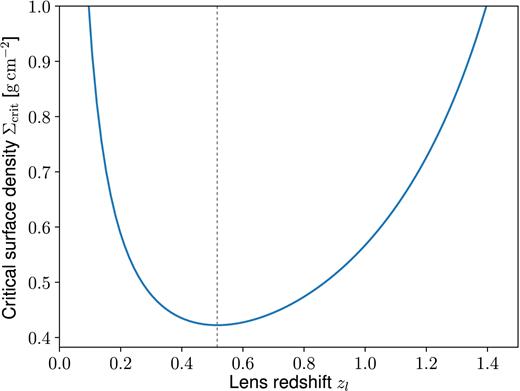
Dependence of the critical surface density for lensing on the lens redshift, computed for a source redshift of |$z$|_s = 2 and cosmological parameters from the Planck 2015 results (Planck Collaboration XIII 2016). The dotted grey line marks the minimum at |$z$| ∼ 0.5.

Open in new tab Download slide

APPENDIX B: SMOOTHED CLUSTER KERNEL

In the following, we briefly outline the steps for solving the convolution integral in equation (33),

\begin{eqnarray*} C(\boldsymbol{\theta }) = \frac{1}{2{\pi} \sigma ^2} \int _{\mathbb {R}^2} \exp \left(- \frac{\Vert \boldsymbol{\theta }- \boldsymbol{\theta }^{\prime } \Vert ^2}{2 \sigma ^2} \right) \Vert \boldsymbol{\theta }^{\prime } \Vert ^{2-q} \, \mathrm{d}^2 \theta ^{\prime }. \end{eqnarray*}

(B1)

Applying the convenient choice of polar coordinates (θ′, ϕ′) such that the orientation of the basis vector |$\boldsymbol{\mathrm{u}_{\theta }}$| coincides with the ϕ′ = 0 axis, the angular integration simply yields a Bessel function of the first kind at order zero:

\begin{eqnarray*} C(\boldsymbol{\theta }) = \frac{\exp \left({- \frac{ \theta ^2}{2 \sigma ^2}} \right)}{\sigma ^2} \int _0^{\infty } I_0 \left(\frac{\theta \theta ^{\prime }}{\sigma ^2} \right) \exp \left(- \frac{\theta ^{\prime 2}}{2 \sigma ^2} \right) \theta ^{\prime \, 3-q} \,\, \mathrm{d}\theta ^{\prime } . \nonumber \\ \end{eqnarray*}

(B2)

It then turns out useful to rewrite the Bessel function I₀ in terms of the confluent hypergeometric limit function ₀F₁ by exploiting the relation (9.63 and 9.6.47, Abramowitz & Stegun 1972):

\begin{eqnarray*} I_{0}(z) = {}_0F_1 \left(; 1; - \frac{z^2}{4} \right). \end{eqnarray*}

(B3)

This simplifies the integral to

\begin{eqnarray*} C(\boldsymbol{\theta }) = \frac{\mathrm{e}^{- \frac{ \theta ^2}{2 \sigma ^2}} }{\sigma ^2} \int _0^{\infty } \exp \left({- \frac{\theta ^{\prime 2} }{2 \sigma ^2} } \right) \theta ^{\prime 3-q} \, {}_0F_1\left(;1; \frac{(\theta \theta ^{\prime })^2}{4 \sigma ^4} \right) \mathrm{d}\theta ^{\prime }. \nonumber \\ \end{eqnarray*}

(B4)

Applying the substitutions |$\smash{\alpha \equiv 2 - \frac{q}{2}}$|⁠, |$\smash{\beta \equiv 1}$| and |$\smash{z \equiv \theta ^2/(2 \sigma ^2)}$|⁠, the remaining expression can be identified as an integral representation of the confluent hypergeometric function ₁F₁ (6.5.1, Magnus, Oberhettinger & Soni 1966):

\begin{eqnarray*} _1F_1(\alpha ; \beta ; z) = \frac{1}{\Gamma (\alpha)} \int _0^{\infty } \mathrm{e}^{-x} \, x^{\alpha -1} \, {}_0F_1(;\beta ; zx) \,\,\mathrm{d}x. \,\,\,\, \end{eqnarray*}

(B5)

This representation is valid for ℜ(α) > 0 and thus q < 4, which is true for all cases we consider (cf. Section 3.3).

Both the integral and the exponential prefactor in equation (B4) can be replaced by a single confluent hypergeometric function if applying Kummer’s transformation rule (6.12, Magnus et al. 1966):

\begin{eqnarray*} \mathrm{e}^{x} \, {}_1F_1(\alpha ; \beta ;-x) = {}_1F_1(\beta - \alpha ; \beta ;x). \end{eqnarray*}

(B6)

With this, the result in equation (33) follows immediately:

\begin{eqnarray*} C(\boldsymbol{\theta }) = \frac{2^{1- \frac{q}{2}}}{\sigma ^{q-2}} \, \Gamma \left(2- \frac{q}{2} \right) {}_1 F_1 \bigg (\frac{q}{2} - 1; 1; -\frac{\theta ^2}{2 \sigma ^2} \bigg). \end{eqnarray*}

(B7)

APPENDIX C: CRITICAL CURVE SHAPE PARAMETERS

The orientation ϕ and the principal axis lengths a and b are defined by (Hu 1962; Stobie 1986)

\begin{eqnarray*} a^2 = 2 \left(\mu _{20} + \mu _{02} \right) + 2 \sqrt{ 4 \mu _{11}^2 + (\mu _{20} - \mu _{02})^2 }; \end{eqnarray*}

(C1)

\begin{eqnarray*} b^2 = 2 \left(\mu _{20} + \mu _{02} \right) - 2 \sqrt{ 4 \mu _{11}^2 + (\mu _{20} - \mu _{02})^2 }; \end{eqnarray*}

(C2)

\begin{eqnarray*} \phi = \frac{1}{2} \arctan \left(\frac{2 \mu _{11}}{\mu _{20} - \mu _{02}} \right). \end{eqnarray*}

(C3)

Here, the normalized centred second-order image moment is defined by

\begin{eqnarray*} \mu _{pq} = \frac{1}{A} \int _{\partial A} (\theta _1 - \bar{\theta }_1)^p \, (\theta _2 - \bar{\theta }_2)^q \,\, \mathrm{d} s, \end{eqnarray*}

(C4)

and the centroid is given by

\begin{eqnarray*} \boldsymbol{\bar{\theta }} = \frac{1}{A} \displaystyle \int _{\partial A} \boldsymbol{\theta }\,\, \mathrm{d} s. \end{eqnarray*}

(C5)

APPENDIX D: PERFORMANCE AND SCALABILITY

For the calibration mode, we measured the average durations of single iterations when using the CPU only and when using GPU acceleration. The average is performed over all sampling iterations (=10⁶) by measuring the total calibration runtime in seconds and dividing by the number of iteration steps. Note that the speed-up of the iterations due to a usage of multiple CPU cores¹⁸ depends on a variety of parameters related to the MCMC sampling procedure. Thus, the values in Table D1 are presented only to give an impression of the order of the involved time-scales; and error bars have been omitted. The duration of a single iteration needs to be kept as short as possible because a large number of MCMC steps are necessary for a reliable estimation of the model parameters. Most of the acceleration is achieved by the reuse of resources in the adaptive MCMC method (cf. Section 5.3), which enables a speed-up by a factor of 10 compared to conventional MCMC methods. The remaining gain from the GPU acceleration contributes only a small part of the speed-up for our set-up due to the unavoidable bottleneck arising from the data transfer between host and GPU device.

Table D1.

Open in new tab

Average duration (in milliseconds) of a single MCMC sampling step for a region of |$\smash{15\,\rm{arcmin} \times 15\,\rm{arcmin}}$| as a function of used CPU cores on our test system.

Number of CPU cores:	1	2	3	4
Time in CPU-only mode (ms):	360	240	170	130
Time in GPU-accelerated mode (ms):	280	190	140	110

Table D1.

Open in new tab

Average duration (in milliseconds) of a single MCMC sampling step for a region of |$\smash{15\,\rm{arcmin} \times 15\,\rm{arcmin}}$| as a function of used CPU cores on our test system.

Number of CPU cores:	1	2	3	4
Time in CPU-only mode (ms):	360	240	170	130
Time in GPU-accelerated mode (ms):	280	190	140	110

For the application mode, we measured the total process runtime averaged over 10 runs. The results are shown in Table D2. Here, the parallel portion is determined primarily by the search area and not expected to change significantly when applying different settings. Thus, we performed millisecond-precision measurements for two different regions – a ‘local cutout’ region of 15 arcmin × 15 arcmin, without temporary buffer, and a |$1\, \mathrm{deg^2}$| region, the latter both with and without temporary extension. Since EasyCritics spends most of its runtime in application mode, we perform a more detailed analysis of the gains that can be expected from the use of parallelization and how this behaviour scales with the problem size. In particular, we evaluate and compare the speed-up for n cores with respect to the single-core performance not only for both regions, but also against the theoretically expected ideal¹⁹ speed-up proposed by Amdahl (1967):

\begin{eqnarray*} S_n = \frac{1}{1 - p + \frac{p}{n}}. \end{eqnarray*}

(D1)

Here, the parallel fraction is set to values derived from direct measurements of the sequential and parallel workloads, which are p = 0.7867 ± 0.0024 for the 15 arcmin × 15 arcmin region, p = 0.9064 ± 0.0023 for the |$1 \, \mathrm{deg^2}$| region, and p = 0.9563 ± 0.0052 for the temporarily extended |$1 \, \mathrm{deg^2}$| region.

Table D2.

Open in new tab

Average runtimes (in seconds) and their statistical uncertainties for application runs on our test system for different region sizes as a function of used CPU cores.

No. of CPU cores:	1	2	3	4
Time for \|$\smash{15\rm{\,arcmin} \times 15\rm{\,arcmin}}$\| (4 tiles, not extended) (s):	5.81 ± 0.18	3.69 ± 0.13	2.84 ± 0.01	2.596 ± 0.003
Time for \|$\smash{\, 1 \, \mathrm{deg}^2}$\| (16 tiles, not extended) (s):	73.35 ± 0.47	39.92 ± 0.35	29.24 ± 0.37	24.65 ± 0.42
Time for \|$\smash{1 \, \mathrm{deg}^2 }$\| (16 tiles, sides extended by 1.5) (s):	160.9 ± 3.9	83.71 ± 0.49	57.40 ± 0.48	41.16 ± 0.35

No. of CPU cores:	1	2	3	4
Time for \|$\smash{15\rm{\,arcmin} \times 15\rm{\,arcmin}}$\| (4 tiles, not extended) (s):	5.81 ± 0.18	3.69 ± 0.13	2.84 ± 0.01	2.596 ± 0.003
Time for \|$\smash{\, 1 \, \mathrm{deg}^2}$\| (16 tiles, not extended) (s):	73.35 ± 0.47	39.92 ± 0.35	29.24 ± 0.37	24.65 ± 0.42
Time for \|$\smash{1 \, \mathrm{deg}^2 }$\| (16 tiles, sides extended by 1.5) (s):	160.9 ± 3.9	83.71 ± 0.49	57.40 ± 0.48	41.16 ± 0.35

Table D2.

Open in new tab

Average runtimes (in seconds) and their statistical uncertainties for application runs on our test system for different region sizes as a function of used CPU cores.

No. of CPU cores:	1	2	3	4
Time for \|$\smash{15\rm{\,arcmin} \times 15\rm{\,arcmin}}$\| (4 tiles, not extended) (s):	5.81 ± 0.18	3.69 ± 0.13	2.84 ± 0.01	2.596 ± 0.003
Time for \|$\smash{\, 1 \, \mathrm{deg}^2}$\| (16 tiles, not extended) (s):	73.35 ± 0.47	39.92 ± 0.35	29.24 ± 0.37	24.65 ± 0.42
Time for \|$\smash{1 \, \mathrm{deg}^2 }$\| (16 tiles, sides extended by 1.5) (s):	160.9 ± 3.9	83.71 ± 0.49	57.40 ± 0.48	41.16 ± 0.35

No. of CPU cores:	1	2	3	4
Time for \|$\smash{15\rm{\,arcmin} \times 15\rm{\,arcmin}}$\| (4 tiles, not extended) (s):	5.81 ± 0.18	3.69 ± 0.13	2.84 ± 0.01	2.596 ± 0.003
Time for \|$\smash{\, 1 \, \mathrm{deg}^2}$\| (16 tiles, not extended) (s):	73.35 ± 0.47	39.92 ± 0.35	29.24 ± 0.37	24.65 ± 0.42
Time for \|$\smash{1 \, \mathrm{deg}^2 }$\| (16 tiles, sides extended by 1.5) (s):	160.9 ± 3.9	83.71 ± 0.49	57.40 ± 0.48	41.16 ± 0.35

The measured speed-ups are shown together with the ideal Amdahl speed-ups in Fig. D1. The error bars presented label the statistical errors. Note that the systematic uncertainties due to factors such as the number or luminosity density of galaxies in the volume or due to numerical settings can be larger. The data suggest a good qualitative agreement with the expectation, although small systematic deviations can be observed, which are most likely due to parallel overheads. As expected, the speed-up improves for a larger area due to the increased parallel portion, indicating a partial weak performance scalability as well. The latter is of interest since EasyCritics is intended for the application to very large data sets.

Figure D1.

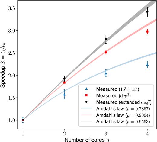
Measured versus ideal speed-up of the computation time for the application mode as a function of CPU cores. The expected ideal speed-up is derived from Amdahl’s law for parallel portions p determined by direct time measurements.

Open in new tab Download slide

This article is published and distributed under the terms of the Oxford University Press, Standard Journals Publication Model (https://dbpia.nl.go.kr/journals/pages/open_access/funder_policies/chorus/standard_publication_model)

Download all slides

Month:	Total Views:
October 2018	5
November 2018	30
December 2018	12
January 2019	9
February 2019	12
March 2019	5
April 2019	9
May 2019	1
June 2019	6
July 2019	2
August 2019	3
September 2019	6
October 2019	6
November 2019	2
December 2019	1
January 2020	1
February 2020	2
March 2020	2
May 2020	1
June 2020	5
July 2020	2
August 2020	2
October 2020	2
December 2020	1
August 2021	1
October 2021	2
December 2021	1
January 2022	3
February 2022	7
March 2022	11
April 2022	35
May 2022	5
June 2022	10
July 2022	17
August 2022	15
September 2022	16
October 2022	16
November 2022	3
December 2022	7
January 2023	2
February 2023	5
March 2023	14
April 2023	9
May 2023	8
June 2023	2
July 2023	10
August 2023	5
September 2023	9
October 2023	2
November 2023	5
December 2023	15
January 2024	13
February 2024	7
March 2024	8
April 2024	6
May 2024	11
June 2024	7
July 2024	13
August 2024	9
September 2024	17
October 2024	17
November 2024	10
December 2024	3
March 2025	31
April 2025	6
May 2025	4

Article Contents

EasyCritics – I. Efficient detection of strongly lensing galaxy groups and clusters in wide-field surveys

Abstract

1 INTRODUCTION

2 OBSERVABLES AND GALAXY SELECTION

3 MASS MODEL

3.1 Stacked mass sheets

3.2 Surface density estimation

3.3 Galaxy-scale subhaloes

3.4 Cluster-scale component

4 STRONG LENSING PRESCRIPTION

4.1 General assumptions

4.2 Effective lens equation

4.3 The lensing potential

4.4 Galaxy-scale subhalo lensing potential

4.5 Cluster-scale halo lensing potential

4.6 Total lensing potential

5 NUMERICAL IMPLEMENTATION

5.1 Parallel computation on mesh grids

5.2 Critical curve recognition

5.3 Parameter calibration

5.4 Performance

6 APPLICATION EXAMPLES

6.1 Selection of known lenses

6.2 Calibrations

6.3 Identification of known lenses

6.4 Impact of redshift uncertainties

7 SUMMARY AND CONCLUSIONS

ACKNOWLEDGEMENTS

Footnotes

REFERENCES

APPENDIX A: REDSHIFT DEPENDENCE OF THE CRITICAL SURFACE DENSITY

APPENDIX B: SMOOTHED CLUSTER KERNEL

APPENDIX C: CRITICAL CURVE SHAPE PARAMETERS

APPENDIX D: PERFORMANCE AND SCALABILITY

Citations

Views

Altmetric

Email alerts

Astrophysics Data System

Citing articles via

Latest

Most Read

Most Cited

This Feature Is Available To Subscribers Only