


ABSTRACT
This paper is the first in a set that analyses the covariance matrices of clustering statistics obtained from several approximate methods for gravitational structure formation. We focus here on the covariance matrices of anisotropic two-point correlation function measurements. Our comparison includes seven approximate methods, which can be divided into three categories: predictive methods that follow the evolution of the linear density field deterministically (ice-cola, peak patch, and pinocchio), methods that require a calibration with N-body simulations (patchy and halogen), and simpler recipes based on assumptions regarding the shape of the probability distribution function (PDF) of density fluctuations (lognormal and Gaussian density fields). We analyse the impact of using covariance estimates obtained from these approximate methods on cosmological analyses of galaxy clustering measurements, using as a reference the covariances inferred from a set of full N-body simulations. We find that all approximate methods can accurately recover the mean parameter values inferred using the N-body covariances. The obtained parameter uncertainties typically agree with the corresponding N-body results within 5 per cent for our lower mass threshold and 10 per cent for our higher mass threshold. Furthermore, we find that the constraints for some methods can differ by up to 20 per cent depending on whether the halo samples used to define the covariance matrices are defined by matching the mass, number density, or clustering amplitude of the parent N-body samples. The results of our configuration-space analysis indicate that most approximate methods provide similar results, with no single method clearly outperforming the others.
1 INTRODUCTION
The statistical analysis of the large-scale structure (LSS) of the Universe is one of the primary tools of observational cosmology. The analysis of the signature of baryon acoustic oscillations (BAO) and redshift-space distortions (RSD) on anisotropic two-point clustering measurements can be used to infer constraints on the expansion history of the Universe (Blake & Glazebrook 2003; Linder 2003) and the redshift evolution of the growth rate of cosmic structures (Guzzo et al. 2008). Thanks to this information, LSS observations have shaped our current understanding of some of the most challenging open problems in cosmology, such as the nature of dark energy, the behaviour of gravity on large scales, and the physics of inflation (e.g. Efstathiou et al. 2002; Cole et al. 2005; Eisenstein et al. 2005; Sánchez et al. 2006, 2012; Anderson et al. 2012, 2014a,b; Alam et al. 2017).
Future galaxy surveys such as Euclid (Laureijs et al. 2011) or the Dark Energy Spectroscopic Instrument (DESI) Survey (DESI Collaboration 2016) will contain millions of galaxies covering large cosmological volumes. The small statistical uncertainties associated with clustering measurements based on these samples will push the precision of our tests of the standard Λ cold dark matter scenario even further. In this context, it is essential to identify all components of the systematic error budget affecting cosmological analyses based on these measurements, as well as to define strategies to control or mitigate them.
A key ingredient to extract cosmological information out of anisotropic clustering statistics is robust estimates of their covariance matrices. In most analyses, covariance matrices are computed from a set of mock catalogues designed to reproduce the properties of a given survey. Ideally, these mock catalogues should be based on N-body simulations, which can reproduce the impact of non-linear structure formation on the clustering properties of a sample with high accuracy. Due to the finite number of mock catalogues, the estimation of the covariance matrix is affected by statistical errors and the resulting noise must be propagated into the final cosmological constraints (Dodelson & Schneider 2013; Taylor, Joachimi & Kitching 2013; Percival et al. 2014; Sellentin & Heavens 2016). Reaching the level of statistical precision needed for future surveys might require the generation of several thousands of mock catalogues. As N-body simulations are expensive in terms of run-time and memory, the construction of a large number of mock catalogues might be infeasible. The required number of realizations can be reduced by means of methods such as resampling the phases of N-body simulations (Hamilton, Rimes & Scoccimarro 2006; Schneider et al. 2011), shrinkage (Pope & Szapudi 2008), calibrating the non-Gaussian contributions of an empirical model against N-body simulations (O’Connell et al. 2016), or covariance tapering (Paz & Sánchez 2015). However, even after applying such methods, the generation of multiple N-body simulations with the required number density and volume to be used for the clustering analysis of future surveys would be extremely demanding.
During the last decades, several approximate methods for gravitational structure formation and evolution have been developed, which allow for a faster generation of mock catalogues; see Monaco (2016) for a review. The accuracy with which these methods reproduce the covariance matrices estimated from N-body simulations must be thoroughly tested to avoid introducing systematic errors or biases on the parameter constraints derived from LSS measurements.
The nIFTy comparison project by Chuang et al. (2015) presented a detailed comparison of major approximate methods regarding their ability to reproduce clustering statistics (two-point correlation function, power spectrum and bispectrum) of halo samples drawn out of N-body simulations. Here, we take the comparison of different approximate methods one step further. We compare the covariance matrices inferred from halo samples obtained from different approximate methods to the corresponding ones derived from full N-body simulations. Furthermore, we also test the performance of the different covariance matrices at reproducing parameter constraints obtained using N-body simulations. We include seven approximate methods, which can be divided into three classes: predictive methods that evolve the linear density field deterministically on Lagrangian trajectories, including ice-cola (Tassev, Zaldarriaga & Eisenstein 2013; Izard, Crocce & Fosalba 2016), peak patch (Bond & Myers 1996), and pinocchio (Monaco, Theuns & Taffoni 2002; Munari et al. 2017), methods that require higher calibration with N-body simulations, such as halogen (Avila et al. 2015) and patchy (Kitaura, Yepes & Prada 2014), and two simpler recipes based on models of the probability distribution function (PDF) of the density fluctuations, the Gaussian recipes of Grieb et al. (2016) and realizations of lognormal density fields constructed using the code of Agrawal et al. (2017). For the predictive and calibrated methods, we generate the same number of halo catalogues as the reference N-body simulations using identical initial conditions. We focus here on the comparison of the covariance matrices of two-point anisotropic clustering measurements in configuration space, considering Legendre multipoles (Padmanabhan & White 2008) and clustering wedges (Kazin, Sánchez & Blanton 2012). Our companion papers, Blot et al. (2018) and Colavincenzo et al. (2018), perform an analogous comparison based on power spectrum and bispectrum measurements.
The structure of the paper is as follows. Section 2 presents a brief description of the reference N-body simulations and the different approximate methods and recipes included in our comparison. In Section 3, we summarize the methodology used in this analysis, including a description of the halo samples that we consider (Section 3.1), our clustering measurements (Section 3.2), the estimation of the corresponding covariance matrices (Section 3.3), and the modelling for the correlation function used to assess the impact of the different methods when estimating parameter constraints (Section 3.4). We present a comparison of the clustering properties of the different halo samples in Section 4.1 and their corresponding covariance matrices in Section 4.2. In Section 4.3, we compare the performance of the different covariance matrices by analysing parameter constraints obtained from representative fits, using as a reference the ones obtained when the analysis is based on N-body simulations. We discuss the results from this comparison in Section 5. Finally, Section 6 presents our main conclusions.
2 APPROXIMATE METHODS FOR COVARIANCE MATRIX ESTIMATES
2.1 Methods included in the comparison
In this comparison project, we included covariance matrices inferred from different approximate methods and recipes, which we compared to the estimates obtained from a set of reference N-body simulations. Approximate methods have recently been revived by high-precision cosmology, due to the need of producing a large number of realizations to compute covariance matrices of clustering measurements. This topic has been reviewed by Monaco (2016), where methods have been roughly divided into two broad classes. ‘Lagrangian’ methods, as N-body simulations, are applied to a grid of particles subject to a perturbation field. They reconstruct the Lagrangian patches that collapse into dark matter (DM) haloes, and then displace them to their Eulerian positions at the output redshift, typically with Lagrangian Perturbation Theory (hereafter LPT). ice-cola, peak patch, and pinocchio fall in this class. These methods are predictive, in the sense that, after some cosmology-independent calibration of their free parameters [that can be thought at the same level as the linking length of friends-of-friends (FoF) halo finders], they give their best reproduction of halo masses and clustering without any further tuning. This approach can be demanding in terms of computing resources and can have high memory requirements. In particular, ice-cola belongs to the class of Particle-Mesh codes; these are in fact N-body codes that converge to the true solution (at least on large scales) for sufficiently small time-steps. As such, Particle-Mesh codes are expected to be more accurate than other approximate methods, at the expense of higher computational costs.
The second class of ‘bias-based’ methods is based on the idea of creating a mildly non-linear density field using some version of LPT, and then populate the density field with haloes that follow a given mass function and a specified bias model. The parameters of the bias model must be calibrated on a simulation, so as to reproduce halo clustering as accurately as possible. The point of strength of these methods is their very low computational cost and memory requirement, that makes it possible to generate thousands of realizations in a simple workstation, and to push the mass limit to very low masses. This is however achieved at the cost of lower predictivity, and need of recalibration when the sample selection changes. halogen and patchy fall in this category.
In the following, we will refer to the two classes as ‘predictive’ and ‘calibrated’ models. All approximate methods used here have been applied to the same set of 300 initial conditions (ICs) of the reference N-body simulations, so as to be subject to the same sample variance; as a consequence, the comparison, though limited to a relatively small number of realizations, is not affected by sample variance.
Additionally, we included in the comparison two simple recipes for the shape of the PDF of the density fluctuations, a Gaussian analytic model that is only valid in linear theory and a lognormal model. The latter was implemented by generating 1000 catalogues of ‘haloes’ that Poisson-sample a lognormal density field; in this test case, we do not match the ICs with the reference simulations, and use a higher number of realizations to lower sample variance.
2.2 Reference N-body halo catalogue: Minerva
Our reference catalogues for the comparison of the different approximate methods is derived from a set of 300 N-body simulations called Minerva, which were performed using gadget-3 (last described in Springel 2005). To the first set of 100 realizations, which is described in more detail in Grieb et al. (2016) and was used in the recent BOSS analyses by Sánchez et al. (2017) and Grieb et al. (2017), 200 new independent realizations were added, which were generated with the same set-up as the first simulations. The ICs were derived from second-order Lagrangian perturbation theory (2LPT) and use the cosmological parameters that match the best-fitting results of the WMAP |$+$| BOSS DR9 analysis by Sánchez et al. (2013) at a starting redshift |$z$|ini = 63. Each realization is a cubic box of side length |$L_{\text{box}} =1.5\, h^{-1}$| Gpc with 10003 DM particles and periodic boundary conditions. For the approximate methods described in the following sections we use the same box size and exactly the same ICs for each realization as in the Minerva simulations. Haloes were identified with a standard FoF algorithm at a snapshot of the simulations at z = 1.0. FoF haloes were then subject to the unbinding procedure provided by the subfind code (Springel et al. 2001), where particles with positive total energy are removed and haloes that were artificially linked by FoF are separated. Given the particle mass resolution of the Minerva simulations, the minimum halo mass is 2.667 × 10¹² h−1 M|${\odot}$|.
2.3 Predictive methods
2.3.1 ice-cola
ice-cola (Izard et al. 2016; Izard, Fosalba & Crocce 2018) is a modification of the parallel version of cola developed in Koda et al. (2016) that produces all-sky light-cone catalogues on-the-fly. Izard et al. (2016) presented an optimal configuration for the production of accurate mock halo catalogues and Izard et al. (2018) explains the light-cone production and the modelling of weak lensing observables.
Mock halo catalogues were produced with ice-cola placing 30 time-steps between an initial redshift of |$z$|i = 19 and |$z$| = 01 and forces were computed in a grid with a cell size three times smaller than the mean inter-particle separation distance. For the FoF algorithm, a linking length of b = 0.2 was used. Each simulation reached redshift 0 and used 200 cores for 20 min in the MareNostrum3 supercomputer at the Barcelona Supercomputing Center,2 consuming a total of 20 CPU kh for the 300 realizations.
2.3.2 PEAK PATCH
From each of the 300 initial density field maps of the Minerva suite, we generate halo catalogues following the peak patch approach initially introduced by Bond & Myers (1996). In particular, we use a new massively parallel implementation of the peak patch algorithm to create efficient and accurate realizations of the positions and peculiar velocities of DM haloes (Stein, Alvarez & Bond 2018). The peak patch approach is essentially a Lagrangian space halo finder that associates haloes with the largest regions that have just collapsed by a given time. The pipeline can be separated into four subprocesses: (1) the generation of a random linear density field with the same phases and power spectrum as the Minerva simulations; (2) identification of collapsed regions using the homogeneous ellipsoidal collapse approximation; (3) exclusion and merging of the collapsed regions in Lagrangian space; and (4) assignment of displacements to these haloes using 2LPT.
The identification of collapsed regions is a key step of the algorithm. The determination of whether any given region will have collapsed or not is made by approximating it as an homogeneous ellipsoid, the fate of which is determined completely by the principal axes of the deformation tensor of the linear displacement field (i.e. the strain) averaged over the region. In principle, the process of finding these local mass peaks would involve measuring the strain at every point in space, smoothed on every scale. However, experimentation has shown that equivalent results can be obtained by measuring the strain around density peaks found on a range of scales.3 This is done by smoothing the field on a series of logarithmically spaced scales with a top-hat kernel, from a minimum radius of Rf,min = 2alatt, where alatt is the lattice spacing, to a maximum radius of |$R_{f,{\rm max}} = 40\, {\rm Mpc}$|, with a ratio of 1.2. For each candidate peak, we then find the largest radius for which a homogeneous ellipsoid with the measured mean strain would collapse by the redshift of interest. If a candidate peak has no radius for which a homogeneous ellipsoid with the measured strain would have collapsed, then that point is thrown out. Each candidate point is then stored as a peak patch at its location with its radius. We then proceed down through the filter bank to all scales and repeat this procedure for each scale, resulting in a list of peak patches which we refer to as the unmerged catalogue.
The next step is to account for exclusion, an essential step to avoid double counting of matter, since distinct haloes should not overlap, by definition. We choose here to use binary exclusion (Bond & Myers 1996). Binary exclusion starts from a ranked list of candidate peak patches sorted by mass or, equivalently, Lagrangian peak patch radius. For each patch we consider every other less massive patch that overlaps it. If the smaller patch is outside of the larger one, then the radius of the two patches is reduced until they are just touching. If the centre of the smaller patch is inside the large one, then that patch is removed from the list. This process is repeated until the least massive remaining patch is reached.
Finally, we move haloes according to 2LPT using displacements computed at the scale of the halo.
This method is very fast: each realization ran typically in 97 s on 64 cores of the GPC supercomputer at the SciNet HPC Consortium in Toronto (1.72 h in total). It allows to get accurate – and fast – halo catalogues without any calibration, achieving high precision on the mass function typically for masses above a few |$10^{13} \, \mathrm{M}_{\odot }$|.
2.3.3 PINOCCHIO
The PINpointing Orbit Crossing Collapsed HIerarchical Objects (pinocchio) code (Monaco et al. 2002) is based on the following algorithm.
A linear density contrast field is generated in Fourier space, in a way similar to N-body simulations. As a matter of fact, the code version used here implements the same loop in k-space as the initial condition generator (N-GenIC) used for the simulations, so the same realization is produced just by providing the code with the same random seed. The density is then smoothed using several smoothing radii. For each smoothing radius, the code computes the time at which each grid point (particle) is expected to get to the highly non-linear regime. The dynamics of grid points, as mass elements, is treated as the collapse of a homogeneous ellipsoid, whose tidal tensor is given by the Hessian of the potential at that point. Collapse is defined as the time at which the ellipsoid collapses on the first axis, going through orbit crossing and into the highly non-linear regime; this is a difference with respect to peak patch, where the collapse of extended structures is modelled. The equations for ellipsoidal collapse are solved using third-order Lagrangian perturbation theory (3LPT). Following the ideas behind excursion-sets theory, for each particle we consider the earliest collapse time as obtained by varying the smoothing radius.
Collapsed particles are then grouped together using an algorithm that mimics the hierarchical assembly of haloes: particles are addressed in chronological order of collapse time; when a particle collapses the six nearest neighbours in the Lagrangian space are checked, if none has collapsed yet then the particle is a peak of the inverse collapse time (defined as F = 1/Dc, where Dc = D(tc) is the growth rate at the collapse time) and it becomes a new halo of one particle. If the collapsed particle is touching (in the Lagrangian space) a halo, then both the particle and the halo are displaced using LPT, and if they get ‘near enough’ the particle is accreted to the halo, otherwise it is considered as a ‘filament’ particle, belonging to the filamentary network of particles that have suffered orbit crossing but do not belong to haloes. If a particle touches two haloes, then their merging is decided by moving them and checking whether they get again ‘near enough’. Here, ‘near enough’ implies a parametrization that is well explained in the original papers (see Munari et al. 2017, for the latest calibration). This results in the construction of haloes together with their merger histories, obtained with continuous time sampling. Haloes are then moved to the final position using 3LPT. The so-produced haloes have discrete masses, proportional to the particle mass Mp, as the haloes found in N-body simulations. To ease the procedure of number density matching described below in Section 3, halo masses were made continuous using the following procedure. It is assumed that a halo of N particles has a mass that is distributed between N × Mp and (N|$+$| 1) × Mp, and the distribution is obtained by interpolating the mass function as a power law between two values computed in successive bins of width Mp. This procedure guarantees that the cumulative mass function of haloes of mass >N × Mp does not change, but it does affect the differential mass function.
We use the latest code version presented in Munari et al. (2017), where the advantage of using 3LPT is demonstrated. No further calibration was required before starting the runs. That paper presents scaling tests of the massively parallel version V4.1 and timings. The 300 runs were produced in the GALILEO@CINECA Tier-1 facility, each run required about 8 min on 48 cores.
2.4 Calibrated methods
2.4.1 HALOGEN
halogen (Avila et al. 2015) is an approximate method designed to generate halo catalogues with the correct two-point correlation function as a function of mass. It constructs the catalogues following four simple steps:
Generate a 2LPT DM field, and distribute their particles on a grid with cell size lcell.
Draw halo masses Mh from an input halo mass function (HMF).
Place the halo masses (from top to bottom) in the cells with a probability that depends on the cell density and the halo mass |$P\propto \rho _{\rm cell}^{\ \ \alpha (M_\mathrm{ h})}$|. Within cells we choose random particles to assign the halo position. We further ensure mass conservation within cells and avoid halo overlap.
Assign halo velocities from the particle velocities, with a velocity bias factor: vhalo = fvel(Mh) · vpart
Following the study in Avila et al. (2015), we fix the cell size at |$l_{\rm cell}=5\, h^{-1}\, {\rm Mpc}$|. In this paper, we take the input HMF from the mean of the 300 Minerva simulations, but in other studies analytical HMF have been used. The parameter α(Mh) controls the clustering as a function of halo mass and has been calibrated using the two-point function from the Minerva simulations in logarithmic mass bins (Mh = 1.06 × 10¹³, 2.0 × 10¹³, 4.0 × 10¹³, 8.0 × 10¹³, |$1.6\times 10^{14}\, h^{-1}\, \mathrm{M}_{ {\odot} }$|). The factor f(Mh) is also tuned to match the variance of the halo velocities from the N-body simulations.
halogen is a code that advocates for the simplicity and low needs of computing resources. The fact that it does not resolve haloes (i.e. using a halo finder), allows to probe low halo masses while keeping low the computing resources. This has the disadvantage of needing to introduce free parameters. However, halogen only needs one clustering parameter α and one velocity parameter fvel, making the fitting procedure simple.
2.4.2 PATCHY
The patchy code (Kitaura et al. 2014, 2015) relies on modelling the large-scale density field with an efficient approximate gravity solver, which is populated with the halo density field using a non-linear, scale dependent, and stochastic biasing description. Although it can be applied to directly paint the galaxy distribution on the density mesh (see Kitaura et al. 2016).
The gravity solver used in this work is based on Augmented Lagrangian Perturbation Theory (ALPT; Kitaura & Heß 2013), fed with the same ICs as those implemented in the Minerva simulations. In the ALPT model, 2LPT is modified by employing a spherical collapse model on small comoving scales, splitting the displacement field into a long- and a short-range component. Better results can in principle be obtained using a Particle-Mesh gravity solver at a higher computational cost (see Vakili et al. 2017).
Once the DM density field is computed, a deterministic bias relating it to the expected number density of haloes is applied. This deterministic bias model consists of a threshold, an exponential cut-off, and a power-law bias relation. The number density is fixed by construction using the appropriate normalization of the bias expression.
The patchy code then associates the number of haloes in each cell by sampling from a negative binomial distribution modelling the deviation from Poissonity with an additional stochastic bias parameter.
In order to provide peculiar velocities, these are split into a coherent and a quasi-virialized component. The coherent flow is obtained from ALPT and the dispersion term is sampled from a Gaussian distribution assuming a power law with the local density.
The masses are associated with the haloes by means of the hadron code (Zhao et al. 2015). In this approach, the masses coming from the N-body simulation are classified in different density bins and in different cosmic web types (knots, filaments, sheets, and voids) and their distribution information is extracted. Then hadron uses this information to assign masses to haloes belonging to mock catalogues. This information is independent of ICs, meaning it will be the same for each of the 300 Minerva realizations.
We used the MCMC python wrapper published by Vakili et al. (2017) to infer the values of the bias parameters from Minerva simulations using one of the 300 random realizations. Once these parameters are fixed one can produce all of the other mock catalogues without further fitting. The patchy mocks were produced using a down-sampled white noise of 5003 instead of the 10003 original Minerva ones with an effective cell side resolution of |$3\, h^{-1}\, {\rm Mpc }$| to produce the DM field.
2.5 Models of the density PDF
2.5.1 Lognormal distribution
The lognormal mocks were produced using the public code presented in Agrawal et al. (2017), which models the matter and halo density fields as lognormal fields, and generates the velocity field from the matter density field, using the linear continuity equation.
To generate a lognormal field |$\delta (\boldsymbol x)$|, a Gaussian field |$G(\boldsymbol x)$| is first generated, which is related to the lognormal field as |$\delta (\boldsymbol x) = \mathrm{ e}^{-\sigma ^2_G+G(\boldsymbol x)}-1$| (Coles & Jones 1991). The pre-factor with the variance |$\sigma ^2_G$| of the Gaussian field |$G(\boldsymbol x)$| ensures that the mean of |$\delta (\boldsymbol x)$| vanishes. Because different Fourier modes of a Gaussian field are uncorrelated, the Gaussian field |$G(\boldsymbol x)$| is generated in Fourier space. The power spectrum of |$G(\boldsymbol x)$| is found by Fourier transforming its correlation function ξG(r), which is related to the correlation function ξ(r) of the lognormal field |$\delta (\boldsymbol x)$| as ξG(r) = ln[1 |$+$| ξ(r)] (Coles & Jones 1991). Having generated the Gaussian field |$G(\boldsymbol x)$|, the code transforms it to the lognormal field |$\delta (\boldsymbol x)$| using the variance |$\sigma ^2_G$| measured from |$G(\boldsymbol x)$| in all cells.
In practice, we use the measured real-space matter power spectrum from Minerva and Fourier transform it to get the matter correlation function. For haloes we use the measured real-space correlation function. We then generate the Gaussian matter and halo fields with the same phases, so that the Gaussian fields are perfectly correlated with each other. Note however, that we use random realizations for these mocks, and so, these phases are not equal to those of the Minerva ICs. We then exponentiate the Gaussian fields, to get matter (|$\delta _m(\boldsymbol x)$|) and halo (|$\delta _g(\boldsymbol x)$|) density fields, following a lognormal distribution.
The expected number of haloes in a cell is given as |$N_g(\boldsymbol x) = \bar{n}_g[1+\delta _g(\boldsymbol x)]V_{\text{cell}}$|, where |$\bar{n}_g$| is the mean number density of the halo sample from Minerva, |$\delta _g(\boldsymbol x)$| is the halo density at position |$\boldsymbol x$|, and Vcell is the volume of the cell. However, this is not an integer. So, to obtain an integer number of haloes from the halo density field, we draw a random number from a Poisson distribution with mean |$N_g(\boldsymbol x)$|, and populate haloes randomly within the cell. The lognormal matter field is then used to generate the velocity field using the linear continuity equation. Each halo in a cell is assigned the three-dimensional velocity of that cell.
Since the lognormal mocks use random phases, we generate 1000 realizations for each mass bin, with the real-space clustering and mean number density measured from Minerva as inputs. Also note that because haloes in this prescription correspond to just discrete points, we do not assign any mass to them. An effective bias relation can still be established using the cross-correlation between the halo and matter fields, or using the input clustering statistics (Agrawal et al. 2017).
The key advantage of using this method is its speed. Once we had the target power spectrum of the matter and halo Gaussian fields, each realization of a 2563 grid, as in Minerva, was produced in 20 s using 16 cores at the RZG in Garching. The resulting catalogues agree perfectly with the Minerva realizations in their real-space clustering as expected. Because we use linear velocities, they also agree with the redshift-space predictions on large scales (Agrawal et al. 2017).
2.5.2 Gaussian distribution
3 METHODOLOGY
3.1 Halo samples
In this section, we describe the criteria used to construct the halo samples on which we base our covariance matrix comparison.
We define two parent halo samples from the Minerva simulations by selecting haloes with masses |$M\ge 1.12\times 10^{13}\, h^{-1}\, \mathrm{M}_{ {\odot} }$| and M ≥ 2.667 × 10¹³ h−1 M|${\odot}$|, corresponding to 42 and 100 DM particles, respectively. We apply the same mass cuts to the catalogues produced by the approximated methods included in our comparison. We refer to the resulting samples as ‘mass1’ and ‘mass2’.
Note that the patchy and lognormal catalogues do not have mass information for individual objects and match the number density and bias of the parent samples from Minerva by construction. The Gaussian model predictions are also computed for the specific clustering amplitude and number density as the mass1 and mass2 samples. For the other approximate methods, the samples obtained by applying these mass thresholds do not reproduce the clustering and the shot noise of the corresponding samples from Minerva. These differences are in part caused by the different applied methods for identifying or assigning haloes, e.g. peak patch uses spherical overdensities in Lagrangian space to define halo masses while most other methods are closer to FoF masses, as described in Section 2. Therefore, for the ice-cola, halogen, peak patch, and pinocchio catalogues we also define samples by matching number density and clustering amplitude of the halo samples from Minerva. For the number-density-matched samples, we find the mass cuts where the total number of haloes in the samples drawn from each approximate method best matches that of the two parent Minerva samples. We refer to these samples as ‘dens1’ and ‘dens2’. Analogously, we define bias-matched samples by identifying the mass thresholds for which the clustering amplitude in the catalogues drawn from the approximate methods best agrees with that of the mass1 and mass2 samples from Minerva. More concretely, we define the clustering-amplitude-matched samples by selecting the mass thresholds that minimize the difference between the mean correlation function measurements from the catalogues drawn from the approximate methods and the Minerva parent samples on scales |$40\, h^{-1}\, {\rm Mpc} \lt s \lt 80\, h^{-1}\, {\rm Mpc}$|. We refer to these samples as ‘bias1’ and ‘bias2’.
The mass thresholds defining the different samples, the number of particles corresponding to these limits, their halo number densities, and bias ratios with respect to the Minerva parent samples are listed in Table 1. Note that, as the halo masses of the pinocchio and peak patch catalogues are made continuous for this analysis, the mass cuts defining the density- and bias-matched samples do not correspond to an integer number of particles. Also note for the calibrated methods that the halogen catalogue was calibrated using the input HMF from the mean of the 300 Minerva simulations in logarithmic mass bins for this analysis, whereas the patchy mass samples were calibrated for each mass cut individually. For the case of the halogen catalogue, the selected high-mass threshold lies nearly half way (in logarithmic scale) between two of the mass thresholds of the logarithmic input HMF. This explains why whereas for the first mass cut, bias and number density are matched by construction, that is not the case for the second mass cut. This has the effect that the bias2 sample of the halogen catalogue has 15 per cent fewer haloes than the corresponding Minerva sample. Comparisons of the ratios of the number densities and bias of the different samples drawn from the approximate methods to the corresponding ones from Minerva are shown in Fig. 1. Since the catalogues drawn from lognormal and patchy match the number density and bias of the Minerva parent samples by construction, they are not included in the tables and figures.
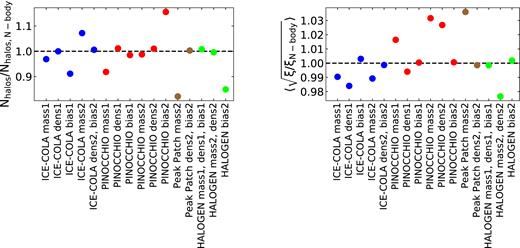
Ratios of the total halo number (left-hand panel) and the clustering amplitude (right-hand panel) of samples drawn from the approximate methods to the corresponding quantity in the Minerva parent samples. By definition, for the dens samples the halo number is matched to the corresponding N-body samples and therefore the corresponding ratio is close to one in the left-hand panel, while the ratios from the bias samples are meant to be close to one in the right-hand panel. For some cases, two or three samples are represented with the same symbol, e.g. ice-cola dens2, bias2 which means that the ice-cola dens2 sample is the same as the ice-cola bias2 sample.
Overview of the different samples, including the mass limits, Mlim, expressed in units of |$h^{-1}\, {\rm M}_{ {\odot} }$|, the corresponding number of particles, Np, the mean number density, |$\bar{n}$|, and the bias ratio to the corresponding Minerva parent sample, 〈(ξapp/ξMin)1/2〉. The sample names ‘mass’, ‘dens’, and ‘bias’, indicate if the samples were constructed by matching the mass threshold, number density, or clustering amplitude of the parent halo samples from Minerva.
| Code | Sample name | |$M_{\rm lim}\left(h^{-1}\,{\rm M}_{ {\odot} }\right)$| | Np | |$\bar{n}\left(h^3\, {\rm Mpc}^{-3}\right)$| | Bias ratio |
|---|---|---|---|---|---|
| Minerva | mass1 | 1.12 × 10¹³ | 42 | 2.12 × 10⁻⁴ | 1.00 |
| Minerva | mass2 | 2.67 × 10¹³ | 100 | 5.42 × 10⁻⁵ | 1.00 |
| ice-cola | mass1 | 1.12 × 10¹³ | 42 | 2.06 × 10⁻⁴ | 0.99 |
| ice-cola | dens1 | 1.09 × 10¹³ | 41 | 2.12 × 10⁻⁴ | 0.98 |
| ice-cola | bias1 | 1.17 × 10¹³ | 44 | 1.93 × 10⁻⁴ | 1.00 |
| ice-cola | mass2 | 2.67 × 10¹³ | 100 | 5.81 × 10⁻⁵ | 0.99 |
| ice-cola | dens2, bias2 | 2.77 × 10¹³ | 104 | 5.45 × 10⁻⁵ | 1.00 |
| halogen | mass1, dens1, bias1 | 1.12 × 10¹³ | 42 | 2.14 × 10⁻⁴ | 1.00 |
| halogen | mass2, dens2 | 2.67 × 10¹³ | 100 | 5.40 × 10⁻⁵ | 0.98 |
| halogen | bias2 | 2.91 × 10¹³ | 109 | 4.61 × 10⁻⁵ | 1.00 |
| peak patcha | mass2 | 2.67 × 10¹³ | 100 | 4.45 × 10⁻⁵ | 1.04 |
| peak patch | dens2, bias2 | 2.35 × 10¹³ | 88.3 | 5.44 × 10⁻⁵ | 1.00 |
| pinocchio | mass1 | 1.12 × 10¹³ | 42 | 1.95 × 10⁻⁴ | 1.02 |
| pinocchio | dens1 | 1.04 × 10¹³ | 39.1 | 2.15 × 10⁻⁴ | 1.00 |
| pinocchio | bias1 | 1.06 × 10¹³ | 39.9 | 2.09 × 10⁻⁴ | 1.00 |
| pinocchio | mass2 | 2.67 × 10¹³ | 100 | 5.35 × 10⁻⁵ | 1.03 |
| pinocchio | dens2 | 2.63 × 10¹³ | 98.6 | 5.48 × 10⁻⁵ | 1.03 |
| pinocchio | bias2 | 2.42 × 10¹³ | 90.7 | 6.27 × 10⁻⁵ | 1.00 |
Note. aAs the halo masses corresponding to our low-mass threshold are not correctly resolved in the peak patch catalogues, only the high-mass threshold (mass2) is considered in this case.
In the following, we refer to all samples corresponding to the first mass limit, mass1, dens1, and bias1 as ‘sample1’, and the samples corresponding to the second mass limit, mass2, dens2, and bias2 as ‘sample2’.
3.2 Clustering measurements in configuration space
3.3 Covariance matrix estimation
We use equation (10) to compute the covariance matrices associated with the measurements of the multipoles and clustering wedges of the halo samples defined in Section 3.1. In order to reduce the noise in these measurements due to the limited number of realizations, we obtain three separate estimates of |$\sf{C}$| from each sample by treating each axis of the simulation boxes as the line-of-sight direction when computing ξ(s, μ). Our final estimates correspond to the average of the covariance matrices measured on the different lines of sight. The Gaussian theoretical covariance matrices were computed for the specific number density and clustering of the halo samples from Minerva. We used as input the model of the two-dimensional power spectrum described in Section 3.4, whose parameters were fitted to reproduce the clustering of parent halo samples.
3.4 Testing the impact of approximate methods for covariance matrix estimates
The constraints on these parameters are sensitive to details in the definition of the likelihood function, such as the way in which the covariance matrix of the measurements is estimated. In order to assess the impact of using approximate methods to estimate |$\sf{C}$|, we perform full-shape fits of anisotropic clustering measurements in configuration space to obtain constraints on α⊥, α∥, and fσ8(|$z$|) assuming the Gaussian likelihood function of equation (9). We compare the constraints obtained when |$\sf{C}$| is estimated from a set of full N-body simulations with the results inferred from the same set of measurements when the covariance matrix is computed using the approximate methods described in Section 2.
Our fits are based on the same model of the full two-dimensional correlation function ξ(μ, s) as in the analyses of the final BOSS galaxy samples (Grieb et al. 2017; Salazar-Albornoz et al. 2017; Sánchez et al. 2017) and the eBOSS DR12 catalogue (Hou et al. 2018). This model includes the effects of the non-linear evolution of density fluctuations based on gRPT (Crocce, Scoccimarro & Blas, in preparation) bias (Chan & Scoccimarro 2012), and RSD (Scoccimarro, in preparation). The only difference between the model implemented in these studies and the one used here is that, since we analyse halo samples instead of galaxies, we do not include the so-called fingers-of-God factor, W∞(k, μ) (see equation 18 in Sánchez et al. 2017). In total, our parameter space contains six free parameters, the BAO and RSD parameters α∥, α⊥, and fσ8, and the nuisance parameters associated with the linear and quadratic local bias, b1 and b2, and the non-local bias |$\gamma _3^-$|. We explore this parameter space by means of the Monte Carlo Markov Chain (MCMC) technique. This analysis set-up matches that of the covariance matrix comparison in Fourier space of our companion paper Blot et al. (2018).
In order to ensure that the model used for the fits has no impact on the covariance matrix comparison, we do not fit the measurements of the Legendre multipoles and wedges obtained from the N-body simulations. Instead, we use our baseline model to construct synthetic clustering measurements, which we then use for our fits. For this, we first fit the mean Legendre multipoles measured from the parent Minerva halo samples using our model and the N-body covariance matrices. We fix all cosmological parameters to their true values and only vary the bias parameters b1, b2, and |$\gamma _3^-$|. We then use the mean values of the parameters inferred from the fits, together with the true values of the cosmological parameters, to generate multipoles and clustering wedges of the correlation function using our baseline model. Fig. 2 shows the mean multipoles and clustering wedges measured from the Minerva halo sample for both mass cuts and the resulting fits. In all cases, our model gives a good description of the simulation results. The parameter values recovered from these fits were also used to compute the input power spectra when computing the Gaussian predictions of |$\sf{C}$|. As these synthetic data are perfectly described by our baseline model by construction, their analysis should recover the true values of the BAO parameters α∥ = α⊥ = 1.0, and the growth-rate parameter fσ8 = 0.4402. The comparison of the parameter values and their uncertainties recovered using different covariance matrices allows us to test the ability of the approximate methods described in Section 2 to reproduce the results obtained when |$\sf{C}$| is inferred from full N-body simulations.
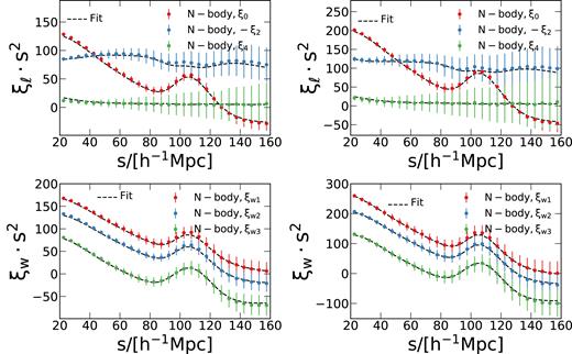
Comparison of the mean correlation function multipoles (upper panels) and clustering wedges (lower panels) of the mass1 and mass2 samples (left-hand and right-hand panels, respectively) drawn from our Minerva N-body simulations, and the model described in Section 3.4. The points with error bars show to the simulation results and the dashed lines correspond to the fit to these measurements. The error bars on the measurements correspond to the dispersion inferred from the 300 Minerva realizations. In all cases, the model predictions show good agreement with the N-body measurements.
4 RESULTS
In this section, we present a detailed comparison of the covariance matrix measurements in configuration space obtained from the approximate methods described in Section 2 and their performance at recovering the correct parameter estimates.
4.1 Two-point correlation function measurements
In order to estimate the covariance matrices from all the samples introduced in Section 3.1, we first measure configuration-space Legendre multipoles and clustering wedges for each sample and in each realization as described in Section 3.2.
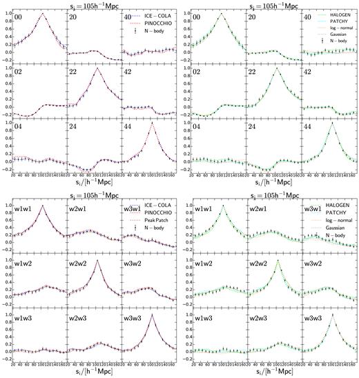
As an illustration of the agreement between the clustering measurements obtained from the approximate methods and the Minerva simulations we focus here on two cases: (i) the multipoles of the density-matched samples for the first mass cut (dens1 samples) and (ii) the clustering wedges of the bias-matched samples for the second mass cut (bias2 samples). As described in Section 3.1, for patchy and the lognormal realizations, the density- and bias-matched samples are identical to the mass-matched samples by construction.
The upper panel of Fig. 3 shows the mean multipole measurements from all realizations for the dens1 samples obtained from the predictive methods ice-cola and pinocchio (left-hand panels) and the calibrated methods halogen, patchy, and the lognormal recipe (right-hand panels). The predictive methods are in excellent agreement with the measurements from the Minerva parent sample, showing only differences of less than 3 per cent for the ice-cola monopole measurements on scales |$ \lt 40\, h^{-1}$| Mpc. The monopole measurements obtained from the calibrated methods and the lognormal model are also in good agreement with the results from Minerva. However, the quadrupole and hexadecapole measurements obtained from halogen and the lognormal samples exhibit deviations of more than 20 per cent on scales |$ \lt 60\, h^{-1}\, {\rm Mpc}$|.

Upper panel: Measurements of the mean multipoles for the density matched samples for the first mass cut (dens1 samples). The first, third, and fifth row show the monople, quadrupole and hexadecapole, respectively. Lower panel: measurements of the mean clustering wedges for the bias matched samples for the second mass cut (bias2 samples). The first, third and fifth row show the transverse, intermediate, and parallel wedge, respectively. Comparison of the measurements drawn from the results of the predictive methods ice-cola and pinocchio (left-hand panels) and the calibrated methods halogen and patchy and the lognormal model (right panels) to the corresponding N-body parent sample. The error bars correspond to the dispersion of the results inferred from the 300 N-body catalogues. The remaining rows show the difference of the mean measurements drawn from the results of the approximate methods to the corresponding N-body measurement.
The lower panel of Fig. 3 shows the mean wedges measurements from all realizations for the bias2 samples obtained from the predictive methods ice-cola, pinocchio, and peak patch (left-hand panels), and for the corresponding samples obtained from calibrated methods halogen, patchy, and the lognormal recipe (right-hand panels). Here, we find that the measurements obtained from the predictive methods and the lognormal model agree well within the error bars with the corresponding Minerva measurements. We notice that the strongest deviations are present in the measurements of the transverse and parallel wedge from the halogen samples, of up to 6 per cent and 20 per cent, respectively, on scales |$ \lt 60\, h^{-1}$| Mpc. The measurements recovered from patchy show deviations ranging between 5 per cent and 10 per cent on small scales.
4.2 Covariance matrix measurements
In this section, we focus on the comparison of the covariance matrix estimates obtained from the different approximate methods, which we computed as described in Section 3.3.
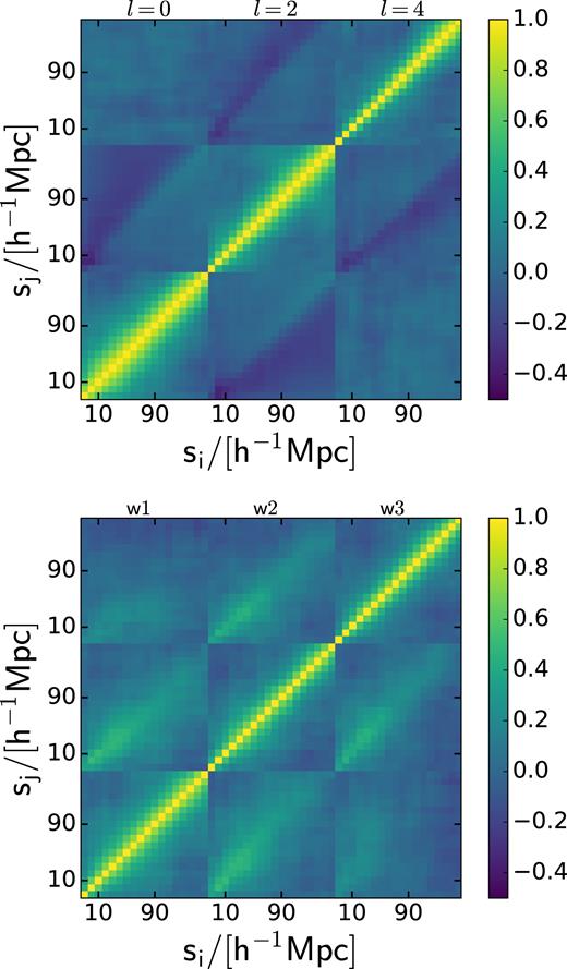
The full correlation matrix inferred from the multipoles of the N-body parent sample for the low-mass cut (mass1, upper panel) and from the clustering wedges of the mass2 N-body parent sample (lower panel).
The estimates of |$\sf{R}$| obtained from the approximate methods are indistinguishable by eye from the ones inferred from the Minerva parent samples and therefore not shown here. Instead, we compare the variances and cuts through the correlation function matrices derived from the different samples. Fig. 5 shows the ratios of the variances drawn from the approximate methods with respect to those of the corresponding Minerva parent catalogues. We focus here on the same example cases as in Section 4.1: the multipoles measured from the dens1 samples, and the clustering wedges measured from the bias2 samples. We notice that in both cases the predictive methods perform better than the calibrated schemes and the PDF-based recipes. On average, the variance from Minerva is recovered within 10 per cent, with a maximum difference of 20 per cent for the variance of the monopole inferred from the pinocchio dens1 sample at scales around |$80\, h^{-1}\, {\rm Mpc}$|. The variances recovered from the other methods show larger deviations, in some cases up to 40 per cent.
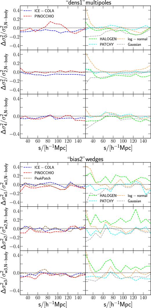
Upper panel: Relative variance of the multipoles of the correlation function measurements from the density matched samples for the first mass cut (dens1 samples).The first, third, and fifth row show the measurements for monople, quadrupole, and hexadecapole, respectively. Lower panel: Relative variance of the clustering wedges of the two-point correlation function for the bias matched samples for the second mass cut (bias2 samples). The first, third, and fifth row show the measurements for transverse, intermediate, and parallel wedge, respectively. Comparison of the relative variance drawn from the results of the predictive methods ice-cola, pinocchio, peak patch (left-hand panel) and halogen, patchy, and the lognormal model (right-hand panel) to the corresponding N-body parent sample.
Cuts at |$s_j = 105\, h^{-1}$| Mpc through the correlation matrices for the two example cases drawn from the results of the approximate methods and the corresponding N-body parent sample. Upper, left panel: Correlation matrices measured from the multipoles of the correlation function drawn from dens1 samples from the predictive methods ice-cola and pinocchio. Upper, right panel: Correlation matrices measured from the multipoles of the correlation function drawn from dens1 samples from the calibrated methods halogen and patchy and the Gaussian and lognormal recipes. Lower, left panel: Correlation matrices measured from the clustering wedges of the correlation function drawn from the bias2 samples from the predictive methods ice-cola, pinocchio, and peak patch. Lower, right panel: Correlation matrices measured from the clustering wedges of the correlation function drawn from bias2 samples from the calibrated methods halogen and p atchy and the Gaussian and lognormal recipes. The error bars are obtained from a jackknife estimate using the 300 Minerva realizations.
| Code | Sample | |$\chi _{\mathrm{ rel}} ^2$| for |$\sf{C}$| from ξ024 | |$\chi _{\mathrm{ rel}} ^2$| for |$\sf{C}$| from ξ|$w$| | |$\chi _{\mathrm{ rel}} ^2$| for |$\sf{R}$| from ξ024 | |$\chi _{\mathrm{ rel}} ^2$| for |$\sf{R}$| from ξ|$w$| | DKL for ξ024 | DKL for ξ|$w$| |
|---|---|---|---|---|---|---|---|
| ice-cola | mass1 | 0.19 | 0.21 | 0.17 | 0.16 | 0.24 | 0.24 |
| ice-cola | dens1 | 0.31 | 0.42 | 0.17 | 0.15 | 0.28 | 0.27 |
| ice-cola | bias1 | 0.20 | 0.11 | 0.19 | 0.19 | 0.27 | 0.27 |
| pinocchio | mass1 | 0.48 | 0.51 | 0.27 | 0.26 | 0.33 | 0.33 |
| pinocchio | dens1 | 0.76 | 0.67 | 0.78 | 0.70 | 0.77 | 0.77 |
| pinocchio | bias1 | 0.23 | 0.20 | 0.24 | 0.22 | 0.28 | 0.29 |
| halogen | mass1 | 1.22 | 0.90 | 1.09 | 0.77 | 1.28 | 1.14 |
| patchy | mass1 | 0.67 | 0.40 | 0.73 | 0.44 | 0.82 | 0.79 |
| Gaussian | mass1 | 2.50 | 2.20 | 2.04 | 0.91 | 0.82 | 1.08 |
| Lognormal | mass1 | 1.76 | 1.09 | 1.31 | 0.97 | 0.96 | 0.98 |
| ice-cola | mass2 | 0.40 | 0.36 | 0.38 | 0.33 | 0.43 | 0.45 |
| ice-cola | dens2 | 0.36 | 0.23 | 0.35 | 0.27 | 0.28 | 0.28 |
| pinocchio | mass2 | 1.03 | 1.20 | 0.44 | 0.41 | 0.46 | 0.44 |
| pinocchio | dens2 | 0.81 | 0.83 | 0.44 | 0.40 | 0.41 | 0.40 |
| pinocchio | bias2 | 0.70 | 0.31 | 0.42 | 0.54 | 0.41 | 0.73 |
| peak patch | mass2 | 1.84 | 2.02 | 0.69 | 0.69 | 1.05 | 1.03 |
| peak patch | dens2 | 0.48 | 0.47 | 0.48 | 0.45 | 0.46 | 0.48 |
| halogen | mass2 | 1.77 | 1.32 | 1.70 | 1.29 | 1.07 | 1.07 |
| halogen | bias2 | 2.24 | 1.76 | 2.06 | 1.59 | 1.28 | 1.32 |
| patchy | mass2 | 1.41 | 1.26 | 1.21 | 0.97 | 0.99 | 1.01 |
| Gaussian | mass2 | 2.02 | 1.77 | 1.75 | 1.03 | 0.78 | 1.14 |
| Lognormal | mass2 | 2.27 | 2.57 | 1.64 | 1.88 | 1.02 | 1.07 |
4.3 Performance of the covariance matrices
For the final validation of the covariance matrices inferred from the different approximate methods, we analyse their performance on cosmological parameter constraints. We perform fits to the synthetic clustering measurements described in Section 3.4, using the estimates of |$\sf{C}$| obtained from the different halo samples and approximate methods. We focus on the constraints on the BAO shift parameters α∥, α⊥, and the growth rate fσ8.
Fig. 7 shows the two-dimensional marginalized constraints in the α⊥–fσ8 plane for the analysis of our two examples cases, the Legendre multipoles measured from the dens1 samples (upper panels), and the clustering wedges recovered from the bias2 samples (lower panel).
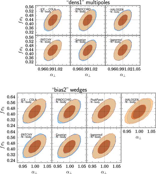
Comparison of the marginalized two-dimensional constraints in the α⊥–fσ8 plane for the analysis of samples from the approximate methods with the corresponding constraints obtained from analysis of the parent Minerva sample. The contours correspond to the 68 per cent and 95 per cent confidence levels.Upper panel: Results from the analysis of the multipoles measured from the dens1 samples. Lower panel: Results from the analysis of the clustering wedges measured from the bias2 samples.
In general, the allowed regions for these parameters obtained using the estimates of |$\sf{C}$| inferred from the different approximate methods (shown by the solid lines) agree well with those obtained using the covariance matrices from Minerva (indicated by the dotted lines in all panels). However, most cases exhibit small deviations, either slightly under- or overestimating the statistical uncertainties. We find that, for all samples and clustering statistics, the mean parameter values inferred using approximate methods are in excellent agreement with the ones from the corresponding N-body analysis, showing differences that are much smaller than their associated statistical errors. The parameter uncertainties recovered using covariances from the approximate methods show differences with respect to the N-body constraints ranging between 0.3 per cent and 8 per cent for the low-mass samples, while most of the results agree within 5 per cent with the N-body results, and between 0.1 per cent and 20 per cent for the high-mass cut, while most of the results agree within 10 per cent with the N-body results. For the comparison of the obtained parameter uncertainties it is important to point out that in our companion paper, Blot et al. (2018) estimate that the statistical limit of our parameter estimation is about 4–5 per cent. Fig. 8 shows the ratios of the marginalized parameter errors drawn from the analysis with the different approximate methods with respect to the N-body results. We observe that for the samples corresponding to the first mass cut, all methods reproduce the N-body errors within 10 per cent for all parameters, and in most cases within 5 per cent corresponding to the statistical limit of our analysis. For the samples corresponding to the second mass cut also most methods reproduce the N-body errors within 10 per cent with exception of the peak patch mass-matched and the halogen bias-matched samples. This might be due to the fact that these two samples have 15–20 per cent less haloes than the corresponding N-body sample.

Comparison of the marginalized error on the parameters α∥, α⊥, and fσ8 which are obtained from the analysis using the covariance matrices from the approximate methods to the corresponding ones from the N-body catalogues. The light grey band indicates a range of |$\pm 10{{\ \rm per\ cent}}$| deviation from a ratio equal to 1. The different panels show the results obtained from the analysis of upper, left panel: the multipoles drawn from the samples corresponding to the first N-body parent sample with the lower mass cut, upper, right panel: the multipoles drawn from the samples corresponding to the second N-body parent sample with the higher mass cut, lower, left panel: the wedges drawn from the samples corresponding to the first N-body sample, lower, right panel: the wedges drawn from the samples corresponding to the second N-body sample.
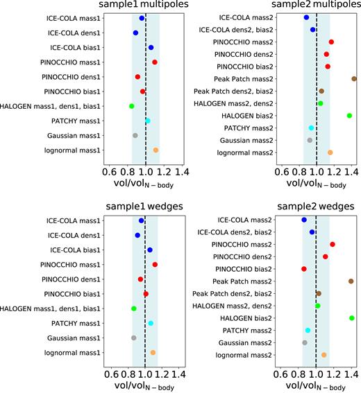
Comparison of the volume ratios between the allowed statistical volumes obtained from the analysis using the covariance matrices from the approximate methods to the corresponding ones from the N-body catalogues. The light grey band indicates a range of |$\pm 10{{\ \rm per\ cent}}$| deviation from a ratio equal to 1. The different panels show the results obtained from the analysis of upper, left panel: the multipoles drawn from the samples corresponding to the first N-body parent sample with the lower mass cut, upper, right panel: the multipoles drawn from the samples corresponding to the second N-body parent sample with the higher mass cut, lower, left panel: the wedges drawn from the samples corresponding to the first N-body sample, lower, right panel: the wedges drawn from the samples corresponding to the second N-body sample.
5 DISCUSSION
In this section, we discuss our results on the allowed parameter space volumes obtained in Section 4.3. Fig. 9 clearly shows that there are significant differences in the volume ratios between samples drawn from the same approximate method when applying different selection criteria to define the halo catalogues. Matching the parent samples from Minerva by mass limit, number density or bias can lead to differences of up to 20 per cent on the obtained results.
For each approximate method, mass limit, and clustering statistic, we identified the best selection criteria for matching to the N-body parent samples. As discussed in Section 3.1, for patchy, lognormal, and the Gaussian model we only have samples characterized by the same mass cuts as the N-body catalogues. The best cases in decreasing order of the accuracy with which the results of the N-body covariances are reproduced are as follows:
Lower mass cut, Legendre multipoles: patchy (V/VMin = 1.02), pinocchio bias matched (V/VMin = 0.97), ice-cola mass matched (V/VMin = 0.96), lognormal (V/VMin = 1.11), Gaussian (V/VMin = 0.88), halogen mass, density, bias matched (V/VMin = 0.85).
Lower mass cut, clustering wedges: pinocchio bias matched (V/VMin = 1.01), ice-cola mass matched (V/VMin = 0.96), patchy (V/VMin = 1.07), lognormal (V/VMin = 1.09), halogen mass, density, bias matched (V/VMin = 0.87), Gaussian (V/VMin = 0.87).
Higher mass cut, Legendre multipoles: ice-cola density matched (V/VMin = 0.96), halogen mass, density matched (V/VMin = 1.04), peak patch density, biased matched (V/VMin = 1.06), patchy (V/VMin = 0.94), Gaussian (V/VMin = 0.92), pinocchio density matched (V/VMin = 1.11), lognormal (V/VMin = 1.16).
Higher mass cut, clustering wedges: halogen mass, density matched (V/VMin = 1.02), ice-cola density matched (V/VMin = 0.97), peak patch density, biased matched (V/VMin = 1.03), patchy (V/VMin = 0.91), lognormal (V/VMin = 1.09), pinocchio density matched (V/VMin = 1.1), Gaussian (V/VMin = 0.87).
For a better illustration, Fig. 10 shows the two-dimensional marginalized constraints on α⊥ and fσ8 obtained from the Legendre multipoles for the low (upper panels) and high (lower panels) mass limits. The different panels show the results obtained from the different approximate methods when the best selection criteria for each case is implemented. The overall agreement with the results derived from the N-body covariances is better in this case than when the same definition is applied to all methods.
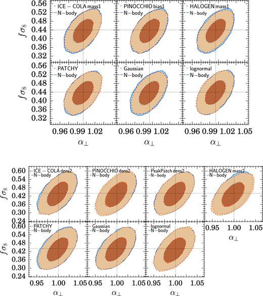
Comparison of the marginalized two-dimensional constraints in the α⊥–fσ8 plane for the multipole analysis using the best choice of matching for each approximate method individually to the corresponding constraints obtained from the N-body analysis. The contours correspond to the 68 per cent and 95 per cent confidence levels.Upper panel: Results for the samples corresponding to the first mass cut. Lower panel: Results for the samples corresponding to the second mass cut.
The best strategy to define the halo samples for a given approximate method is often different for our two mass limits. For example, considering the results from pinocchio, while for our first mass limit the bias-matched halo samples lead to the best agreement with the constraints inferred from the N-body covariances, for the second mass threshold the density-matched samples provide a better performance. Focusing on the results from the multipole analysis, we observe that for the first mass limit patchy, ice-cola, and pinocchio perform slightly better than the other methods. These methods reproduce the statistical volume of the allowed parameter regions obtained using the N-body covariances within 5 per cent while the other methods only reach a 10–15 per cent agreement. For the second mass limit ice-cola, halogen, and peak patch can reproduce the N-body results within 5 per cent, patchy and the Gaussian model within 10 per cent, and pinocchio and the lognormal model within 15 per cent. It is also interesting to note that the order of performance of the methods is slightly different for the multipole and the wedges analysis. For example, the multipole analysis using the patchy covariance matrix leads to a better than 2 per cent agreement with the N-body results, whereas the wedge analysis only reaches 7 per cent.
Our analysis is part of a general comparison project of approximate methods involving also the covariances of power spectrum and bispectrum measurements (Blot et al. 2018; Colavincenzo et al. 2018). The power spectrum analysis of Blot et al. (2018) is more closely related to the one presented here, as it is based on the same baseline model of the two-dimensional power spectrum and explore constraints on the same nuisance and cosmological parameters. The bispectrum covariance analysis of Colavincenzo et al. (2018) is different in terms of the model and the parameter constraints included in the comparison. Both of our companion papers consider the same approximate methods and mass cuts used here, but focus on the abundance-matched samples. A comparison of the results of the three studies shows that the differences between the predictive, calibrated and PDF-based approximate methods are less evident for the correlation function analysis than for the power spectrum and bispectrum. This can be clearly seen by comparing the variations of the statistically allowed volumes recovered from the different approximate methods when applied to the correlation function, power spectrum and bispectrum covariances. Since our companion papers focus on the density-matched samples, we also show the allowed volumes only for the ‘dens’ samples in Fig. 11. The differences between the approximate methods are less evident in configuration space, become more evident for the power spectrum and are strongest for the bispectrum analysis.
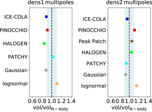
Volume ratios between the allowed statistical volumes obtained from the analysis using the covariance matrices from the approximate methods to the corresponding ones from the N-body catalogues for the density matched samples. The light grey band indicates a range of |$\pm 10{{\ \rm per\ cent}}$| deviation from a ratio equal to 1.
In summary, our results and those of our companion papers indicate that approximate methods can provide robust covariance matrix estimates for cosmological parameter constraints. However, the differences seen between the various recipes, statistics, and selection criteria considered here highlight the importance of performing detailed tests to find the best strategy to draw halo samples from any given approximate method.
6 SUMMARY AND CONCLUSIONS
We have analysed the performance of several approximate methods at providing estimates of the covariance matrices of anisotropic two-point clustering measurements in configuration space. Our analysis is part of a comparison project, including also detailed studies of the covariance matrices of power spectrum and bispectrum measurements, which are summarized in our companion papers Blot et al. (2018) and Colavincenzo et al. (2018), respectively.
Our comparison included seven approximate methods, which we divided into three categories: predictive methods (ice-cola, peak patch, and pinocchio), methods that require calibration with N-body simulations (halogen and patchy), and recipes based on assumptions regarding the shape of the density PDF (lognormal and Gaussian density fields). We compared these methods against the results obtained from the Minerva simulations. We generated sets of 300 halo catalogues using the predictive and calibrated methods, matching the ICs of the reference N-body simulations. For the lognormal predictions we generated a set of 1000 catalogues designed to match the number density and mean correlation function measured from the N-body simulations.
We defined two halo samples from the Minerva simulations by applying mass thresholds corresponding to 42 and 100 DM particles. We then selected different halo samples from the approximate methods by matching the mass threshold, number density and clustering amplitude of the parent samples from the N-body simulations. We estimated the covariance matrices of the Legendre multipoles and clustering wedges corresponding to all halo samples and compared the results with the corresponding ones from the parent catalogues.
Our main comparison was focused on the accuracy with which the covariance matrices inferred from the approximate methods reproduce the cosmological parameter constraints obtained from the N-body results. For this, we first used a model of the two-dimensional power spectrum applied in recent LSS analyses (Grieb et al. 2017; Salazar-Albornoz et al. 2017; Sánchez et al. 2017; Hou et al. 2018) to construct synthetic clustering measurements, and then fitted these data with the same baseline model, using the covariances from the different methods and assuming a Gaussian likelihood function. We analysed the obtained parameter constraints on α∥, α⊥ and fσ8. The mean values obtained from the fits agree perfectly with the N-body results for all the samples. Most methods recover the marginalized N-body parameter errors within 5 per cent for the lower mass cut, which corresponds also to the statistical limit of our analysis, and 10 per cent for the higher mass cut. The comparison of the statistically allowed volumes in the three-dimensional parameter space of α∥, α⊥, and fσ8 shows that the results obtained from any given approximate method by implementing different selection criteria, i.e. by matching the mass, number density, or bias of the parent N-body samples, can differ by up to 20 per cent. Therefore, for each approximate method and mass limit we identified the selection scheme that provided the closest agreement with the results obtained using the estimates of |$\sf{C}$| from the N-body simulations. For the first mass cut, we found that the methods ice-cola, pinocchio, and patchy reproduce the N-body results slightly better than the other methods, with differences of less than 10 per cent in the allowed volumes. The remaining methods show a 10–15 per cent agreement with the N-body results. For the second mass cut, ice-cola, halogen, and peak patch perform the best, recovering the N-body allowed volumes within 5 per cent. The fits using the other methods lead to a 5–15 per cent agreement. It is noteworthy that the simple Gaussian prediction performs similar to the other approximate methods.
We conclude that, with respect to the covariance matrices of configuration-space clustering measurements, there is no clear preference for one of the approximate methods. The predictive methods ice-cola, peak patch, and pinocchio do not outperform the calibrated methods and simpler recipes significantly. The advantage of using the calibrated methods is that they are computationally less expensive. However, the calibration using full N-body simulations can also be challenging and time-consuming. In future studies, we will include additional effects, such as the impact of survey geometry, that will allow us to extend our analysis to assess the impact of applying approximate methods to the analysis of real galaxy surveys.
ACKNOWLEDGEMENTS
This paper and companion papers have benefited of discussions and the stimulating environment of the Euclid Consortium, which is warmly acknowledged.
ML and AGS thank Daniel Farrow, Jiamin Hou, and Francesco Montesano for the useful discussion. ML and AGS acknowledge support from the Transregional Collaborative Research Centre TR33 The Dark Universe of the German Research Foundation (DFG). MC is supported by the Departments of Excellence 2018–2022 Grant awarded by the Italian Ministero dell’Istruzione, dell’Università e della Ricerca (MIUR) (L. 232/2016), by the research grant The Anisotropic Dark Universe Number CSTO161409, funded under the program CSP-UNITO Research for the Territory 2016 by Compagnia di Sanpaolo and University of Torino; and the research grant TAsP (Theoretical Astroparticle Physics) funded by the Istituto Nazionale di Fisica Nucleare (INFN). PM acknowledges support from a FRA2015 grant from MIUR PRIN 2015 Cosmology and Fundamental Physics: illuminating the Dark Universe with Euclid. PM and ES acknowledge support from a FRA2015 grant from MIUR PRIN 2015 Cosmology and Fundamental Physics: illuminating the Dark Universe with Euclid and from Consorzio per la Fisica di Trieste; they are part of the INFN InDark research group. LB acknowledges support from the Spanish Ministerio de Economía y Competitividad (MINECO) grant ESP2015-66861. MC acknowledges support from the Spanish Ramón y Cajal MICINN program. MC has been funded by AYA2015-71825.
CD Vecchia acknowledges support from the MINECO through grants AYA2013-46886, AYA2014-58308, and RYC-2015-18078. SA acknowledges support from the UK Space Agency through grant ST/K00283X/1. ABA acknowledges financial support from MINECO under the Severo Ochoa program SEV-2015-0548. MPI acknowledges support from MINECO under the grant AYA2012-39702-C02-01. PF acknowledges support from MINECO through grant ESP2015-66861-C3-1-R and Generalitat de Catalunya through grant 2017-SGR-885. AI was supported in part by Jet Propulsion Laboratory, California Institute of Technology, under a contract with the National Aeronautics and Space Administration. He was also supported in part by NASA ROSES 13-ATP13-0019, NASA ROSES 14-MIRO-PROs-0064, NASA ROSES 12- EUCLID12-0004, and acknowledges support from the JAE program grant from the Spanish National Science Council (CSIC). RB, SC, and GS are supported by the Canadian Natural Sciences and Engineering Research Council (NSERC). GY acknowledges financial support from MINECO/FEDER (Spain) under research grant AYA2015-63810-P.
The Minerva simulations have been performed and analysed on the Hydra and Euclid clusters at the Max Planck Computing and Data Facility (MPCDF) in Garching.
pinocchio mocks were run on the GALILEO cluster at CINECA thanks to an agreement with the University of Trieste.
ice-cola simulations were run at the MareNostrum supercomputer – Barcelona Supercomputing Center (BSC-CNS, http://www.bsc.es), through the grant AECT-2016- 3-0015.
peak patch simulations were performed on the GPC supercomputer at the SciNet HPC Consortium. SciNet is funded by: the Canada Foundation for Innovation under the auspices of Compute Canada; the Government of Ontario; Ontario Research Fund - Research Excellence; and the University of Toronto.
Numerical computations with halogen were done on the Sciama High-Performance Compute (HPC) cluster which is supported by the ICG, SEPNet, and the University of Portsmouth.
patchy mocks have been computed in part at the MareNostrum supercomputer of the Barcelona Supercomputing Center thanks to a grant from the Red Española de Supercomputación (RES), and in part at the Teide High-Performance Computing facilities provided by the Instituto Tecnológico y de Energías Renovables (ITER, S.A.).
Footnotes
The time-steps were linearly distributed with the scale factor.
This is not to say that a halo found on a given scale corresponds to a peak in the density smoothed on that scale, however, which is only the case when the strain is isotropic and the collapse is spherical. Thus, the use of density peaks as centres for strain measurements and ellipsoidal collapse calculations in the algorithm is only an optimization, to avoid wasting computations measuring the properties of regions of Lagrangian space that are unlikely to collapse in the first place.
