


Abstract
We report the discovery of four transiting hot Jupiters, WASP-147, WASP-160B, WASP-164, and WASP-165 from the WASP survey. WASP-147b is a near Saturn-mass (MP = 0.28MJ) object with a radius of |$1.11 \, {{R}_{J}}$| orbiting a G4 star with a period of 4.6 d. WASP-160Bb has a mass and radius (|$M_p = 0.28 \, {{M}_{J}}$|, |$R_p = 1.09 \, {{R}_{J}}$|) near-identical to WASP-147b, but is less irradiated, orbiting a metal-rich ([Fe/H]* = 0.27) K0 star with a period of 3.8 d. WASP-160B is part of a near equal-mass visual binary with an on-sky separation of 28.5 arcsec. WASP-164b is a more massive (|$M_P = 2.13 \, {{M}_{J}}$|, |$R_p = 1.13 \, {{R}_{J}}$|) hot Jupiter, orbiting a G2 star on a close-in (P = 1.8 d), but tidally stable orbit. WASP-165b is a classical (|$M_p = 0.66 \, {{M}_{J}}$|, |$R_P = 1.26 \, {{R}_{J}}$|) hot Jupiter in a 3.5 d period orbit around a metal-rich ([Fe/H]* = 0.33) star. WASP-147b and WASP-160Bb are promising targets for atmospheric characterization through transmission spectroscopy, while WASP-164b presents a good target for emission spectroscopy.
1 INTRODUCTION
Transiting exoplanets are invaluable objects for study. Not only are both their masses and radii known, but also their transiting configuration opens up a wide range of characterization avenues. We may study the atmospheres of these objects through their transmission and emission spectra (Seager & Sasselov 2000; Charbonneau et al. 2002, 2005), but also measure their orbital alignment (Queloz et al. 2000); see Triaud (2017) for a summary. While over 2700 transiting planets are known to date, 1 only a fraction of these objects are suitable for detailed characterization, as this requires the planet host to be bright and the star/planet size ratio to be favourable.
Ground based transit surveys (e.g. HAT, Bakos et al. 2004; WASP, Pollacco et al. 2006; KELT, Pepper et al. 2007; and MASCARA, Talens et al. 2017) use small-aperture instrumentation to monitor vast numbers of bright stars across nearly the entire sky, sensitive to the ∼1 per cent dips created by transits of close-in giant planets. These hot Jupiters are prime targets for further characterization thanks to their large radii, frequent transits, and extended atmospheres. Indeed, ground-based transit surveys have provided some of the most intensely studied planets to date (e.g. WASP-12b, Hebb et al. 2009; WASP-43b, Hellier et al. 2011; and HAT-P-11b, Bakos et al. 2010).
In this paper, we report the discovery of four additional close-in transiting gas giants by WASP-South, the two Saturn-mass planets WASP-147b and WASP-160Bb, and the two hot Jupiters WASP-164b and WASP-165b. We discuss the observations leading to these discoveries in Section 2, describe their host stars in Section 3, and discuss the individual planetary systems and their place among the known planet population in Section 4 before concluding in Section 5.
2 OBSERVATIONS
WASP-147 (2MASS 23564597-2209113), WASP-160B (2MASS 05504305-2737233), WASP-164 (2MASS 22592962-6026519), and WASP-165 (2MASS 23501932-1704392) were monitored with the WASP-South facility throughout several years between 2006 and 2013. In the case of WASP-160B, the target flux was blended with that of another object (2MASS 05504470-2737050, revealing to be physically associated, see below) in the WASP aperture. The WASP-South instrument consists of an array of 8 cameras equipped with 200mm f/8 Canon lenses on a single mount and is located at SAAO (South Africa). For details on observing strategy, data reduction, and target selection, please refer to Pollacco et al. (2006) and Collier Cameron et al. (2007). Using the algorithms described by Collier Cameron et al. (2006), we identified periodic flux drops compatible with transits of close-in giant planets in the light curves of these four objects. We thus triggered spectroscopic and photometric follow-up observations to determine the nature of the observed dimmings.
2.1 Follow-up spectroscopy
We obtained spectroscopic observations of all four objects using the CORALIE echelle spectrograph at the 1.2 m Euler-Swiss telescope at La Silla. From the spectra, we computed radial velocities (RVs) using the weighted cross-correlation method (Baranne et al. 1996; Pepe et al. 2002). In 2014, the CORALIE spectrograph was upgraded by replacing circular with octagonal fibers, leading to a shift in RV zero-point between observations obtained before and after the exchange. WASP-160B, 164, and 165 were observed only after the upgrade, resulting in a single homogeneous set of RVs for each object. WASP-147 was observed before and after the upgrade, making it necessary to include these observations as two separate data sets in our analysis. For each of the four objects in question, RV variations confirmed the presence of a planet orbiting at the period of the observed transits (see Figs 1–4). The individual RV measurements are listed in Tables 1–4. To exclude stellar activity as the origin of the observed RV variations, we verified that bisector spans and RVs are uncorrelated (Queloz et al. 2001; Pearson coefficients are −0.19 ± 0.16, −0.16 ± 0.19, −0.24 ± 0.22, and 0.06 ± 0.22 for WASP-147, 160B, 164, and 165, respectively). This is illustrated in Fig. 5, where we plot bisector spans against RVs. As both stellar components of the WASP-160AB system fell into the same WASP-South aperture, we could not a priori exclude either of them as the origin of the observed transits. We thus obtained several spectra of WASP-160A, showing no evidence of any large-amplitude RV variability (see Fig. 6).
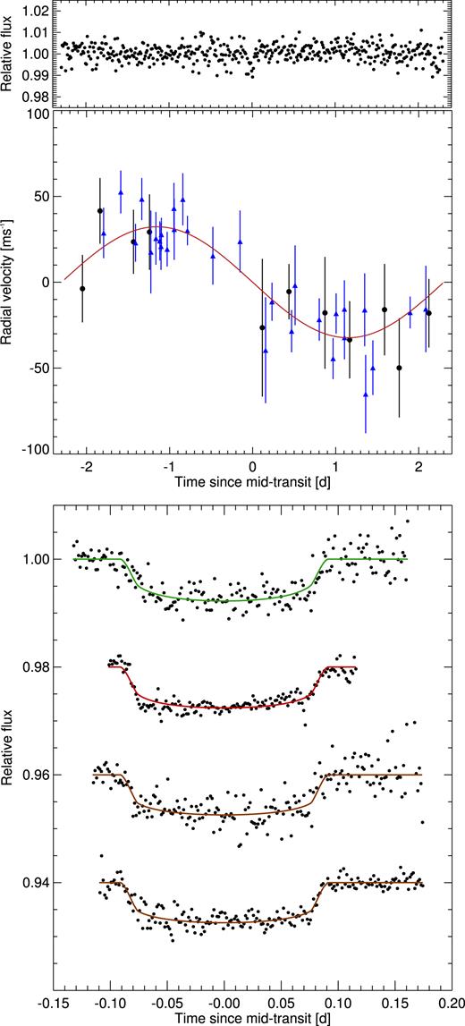
Discovery and follow-up photometry and RVs of WASP-147. Top panel: WASP survey data, phase-folded on the period of WASP-147b and binned per 15 min. Middle panel: CORALIE RV data, where the pre-upgrade data are shown as blue triangles, and the post-upgrade data are shown as black filled circles. Bottom panel: Follow-up transit light curves, corrected for their respective baseline models and binned by two min. They are (from top to bottom): V-band TRAPPIST data of 2014 Nov 5, and r’-band EulerCam data of 2013 Nov 11, and blue-block TRAPPIST data of 2013 Oct 19 and 2013 Sep 26. The systematics seen in the 2013 Nov 11 light curve are due to cloud passages.
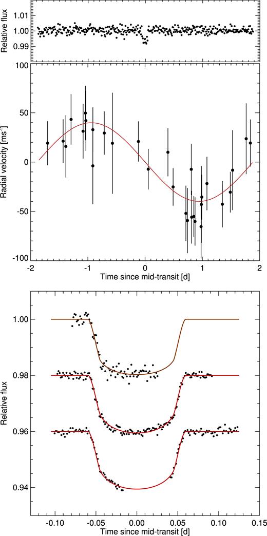
Discovery and follow-up photometry and RVs of WASP-160B. As Fig. 1. The light curves shown are (from top to bottom): I + z’-band TRAPPIST data of 2014 Dec 16, and r’-band EulerCam data of 2015 Dec 26 and 2017 Jan 2. Note that the transit depth in the WASP light curve is reduced due to contamination from WASP-160A.
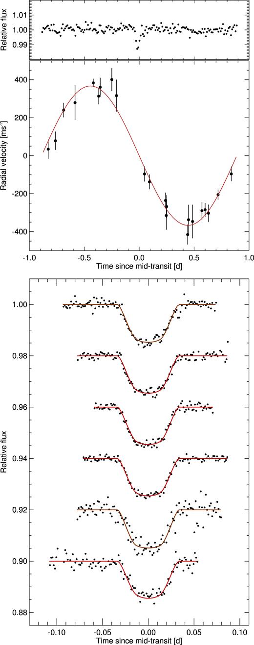
Discovery and follow-up photometry and RVs of WASP-164. As Fig. 1. The light curves shown are (from top to bottom): blue-block TRAPPIST data of 2015 Jun 29, r’-band EulerCam data of 2015 Jul 31, 2015 Aug 16 and 2015 Aug 25, I + z’-band TRAPPIST data of 2016 Sep 10 and and R-band SAAO data of 2016 Oct 16.
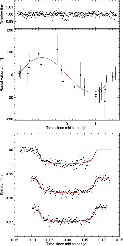
Discovery and follow-up photometry and RVs of WASP-165. As Fig. 1. The light curves shown are (from top to bottom): NGTS-filter EulerCam light curves of 2015 Mar 10, 2016 Sep 17, and 2016 Sep 24.
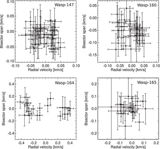
Bisector spans against RV of our targets. The RVs have been corrected for the systemic velocities given in Table 10.
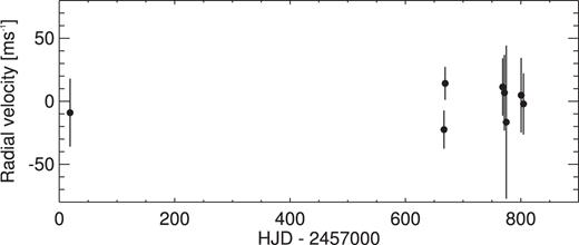
CORALIE RVs of WASP-160A.
RV measurements of WASP-147. Only the first five entries are shown; the full table is available in the online version.
| HJD-2450000 | RV [|${\rm km\, s}^{-1}$|] | error [|${\rm km\, s}^{-1}$|] | bisector [|${\rm km\, s}^{-1}$|] | note |
|---|---|---|---|---|
| 6135.904214 | −1.70365 | 0.02277 | −0.01228 | pre-upgrade |
| 6137.920709 | −1.62092 | 0.02408 | −0.01027 | pre-upgrade |
| 6157.712465 | −1.67809 | 0.03085 | 0.01114 | pre-upgrade |
| 6158.661748 | −1.65414 | 0.01670 | 0.01027 | pre-upgrade |
| 6508.712267 | −1.65458 | 0.02119 | 0.00580 | pre-upgrade |
RV measurements of WASP-160B. Only the first five entries are shown; the full table is available in the online version.
| HJD-2450000 | RV [|${\rm km\, s}^{-1}$|] | error [|${\rm km\, s}^{-1}$|] | bisector [|${\rm km\, s}^{-1}$|] |
|---|---|---|---|
| 7011.653767 | −6.16374 | 0.02709 | 0.03897 |
| 7016.726245 | −6.12609 | 0.03159 | −0.07226 |
| 7019.639217 | −6.15020 | 0.04051 | −0.03465 |
| 7037.692732 | −6.20130 | 0.03296 | −0.01686 |
| 7038.718708 | −6.11831 | 0.03588 | −0.04539 |
RV measurements of WASP-164. Only the first five entries are shown; the full table is available in the online version.
| HJD-2450000 | RV [|${\rm km\, s}^{-1}$|] | error [|${\rm km\, s}^{-1}$|] | bisector [|${\rm km\, s}^{-1}$|] |
|---|---|---|---|
| 7185.833271 | 12.66344 | 0.06016 | 0.00090 |
| 7191.863118 | 11.92547 | 0.07861 | 0.18480 |
| 7192.836522 | 12.62296 | 0.04957 | −0.08816 |
| 7193.822033 | 11.95951 | 0.04570 | 0.05691 |
| 7200.871113 | 11.97277 | 0.04621 | 0.08865 |
RV measurements of WASP-165. Only the first five entries are shown; the full table is available in the online version.
| HJD-2450000 | RV [|${\rm km\, s}^{-1}$|] | error [|${\rm km\, s}^{-1}$|] | bisector [|${\rm km\, s}^{-1}$|] |
|---|---|---|---|
| 7014.541384 | 25.74712 | 0.02309 | 0.06029 |
| 7016.541690 | 25.56122 | 0.02932 | 0.03612 |
| 7178.889363 | 25.65436 | 0.05627 | 0.08364 |
| 7187.897899 | 25.70129 | 0.03835 | 0.05943 |
| 7190.895590 | 25.66115 | 0.04947 | −0.00215 |
2.2 Follow-up photometry
We obtained several high-precision transit light curves for each of our targets to obtain an improved measurement of the transit shape and depth. The facilities we used for this purpose were EulerCam at the 1.2 m Euler-Swiss telescope (Lendl et al. 2012), the 0.6 m TRAPPIST-South telescope (Gillon et al. 2011; Jehin et al. 2011), and the SAAO 1.0 m telescope. In all cases, we extracted light curves of the transit events using relative aperture photometry, while iteratively selecting reference stars and aperture sizes to minimize the final light curve RMS. Having an on-sky separation of 28.478948 ± 2.5 × 10⁻⁵ arcsec, both stellar components of the WASP-160 system were well-separated in these observations, confirming the fainter star, WASP-160B as the origin of the transit feature. Details on all photometric follow-up observations are listed in Table 5. The resulting light curves are shown in Figs 1–4.
Summary of photometric follow-up observations together with the preferred baseline model, noise correction factors, and the light curves’ RMS per 5 min bin. The notation of the baseline models, p(ji), refers to a polynomial of degree i in parameter j. Filter ranges: |$\lambda _{\mathit {blue-block}} \gt 500$| nm, |$\lambda _{\mathit {NGTS}} = [500 - 900]$| nm, Wheatley et al. (2018).
| Date | Instrument | Filter | Baseline | βr | β|$w$| | RMS5min [ppm] |
|---|---|---|---|---|---|---|
| WASP-147 | ||||||
| 2014 Nov 5 | TRAPPIST-South | V | p(t2) | 1.22 | 1.22 | 1419 |
| 2013 Nov 11 | EulerCam | r’ | p(t2) + p(FWHM1) | 2.42 | 1.64 | 1020 |
| 2013 Oct 19 | TRAPPIST-South | blue-block | p(t2) | 1.33 | 0.98 | 1682 |
| 2013 Sep 26 | TRAPPIST-South | blue-block | p(t2) | 2.02 | 0.81 | 900 |
| WASP-160B | ||||||
| 2014 Dec 16 | TRAPPIST-South | I + z’ | p(t2) | 1.16 | 0.99 | 1091 |
| 2015 Dec 26 | EulerCam | r’ | p(t2) | 1.50 | 1.06 | 469 |
| 2017 Jan 2 | EulerCam | r’ | p(t2) | 1.92 | 1.08 | 628 |
| WASP-164 | ||||||
| 2015 Jun 29 | TRAPPIST-South | blue-block | p(t2) | 1.58 | 0.89 | 1070 |
| 2015 Jul 31 | EulerCam | r’ | p(t2) + p(sky1) | 1.21 | 1.52 | 1103 |
| 2015 Aug 16 | EulerCam | r’ | p(t2) | 1.00 | 1.45 | 616 |
| 2015 Aug 25 | EulerCam | r’ | p(t2) + p(xy1) | 1.09 | 1.31 | 503 |
| 2016 Sep 10 | TRAPPIST-South | I + z’ | p(t2) + p(FWHM2) + p(xy1) | 1.01 | 2.81 | 1301 |
| 2016 Oct 16 | SAAO 1m | R | p(t2) | 1.61 | 0.85 | 1302 |
| WASP-165 | ||||||
| 2015 Mar 10 | EulerCam | NGTS | p(t2) + p(FWHM1) | 1.52 | 1.60 | 623 |
| 2016 Sep 17 | EulerCam | NGTS | p(t2) + p(FWHM1) | 1.32 | 1.46 | 626 |
| 2016 Sep 24 | EulerCam | NGTS | p(t2) + p(FWHM1) | 1.98 | 1.41 | 559 |
3 STELLAR PARAMETERS
3.1 Spectral analysis
The individual CORALIE spectra for each star were co-added in order to provide a spectrum for analysis. Using methods similar to those described by Doyle et al. (2013), for each star we determined the effective temperature (Teff), surface gravity (log g), stellar metallicity ([Fe/H]), and projected stellar rotational velocity (|$v$|rotsin i*). In determining |$v$|rotsin i* we assumed a macroturbulent velocity using the calibration given by Doyle et al. (2014). For WASP-160B and WASP-165, the |$v$|rotsin i* values are consistent with zero and that of WASP-147 can be considered an upper limit, as it is close to the resolution limit of the CORALIE spectrograph. If, however, a zero macroturbulent velocity is used, we obtain |$v$|rotsin i* values of 3.1 ± 0.5, 0.7 ± 0.6, and 2.8 ± 0.6 km s−1 for WASP-147, WASP-160B, and WASP-165, respectively.
The parameters for WASP-164 are relatively poorly determined, as the signal-to-noise ratio of the merged spectrum for WASP-164 is very low (≲20:1). The |$v$|rotsin i* is consistent with zero, but very poorly determined and the Lithium 670.8 nm line might be present, but we cannot be sure due to the quality of the spectrum. The stellar parameters found are summarized in Table 6.
Basic properties and stellar parameters of the planet hosts based on spectroscopic analysis, evolutionary models and photometric variability.
| Parameter | WASP-147 | WASP-160B | WASP-164 | WASP-165 |
|---|---|---|---|---|
| Basic parameters | ||||
| RA (J2000) | 23 56 45.97 | 05 50 43.06 | 22 59 29.62 | 23 50 19.33 |
| DEC (J2000) | −22 09 11.39 | −27 37 23.39 | −60 26 51.97 | −17 04 39.26 |
| UCAC4 B [mag] | 12.96 ± 0.04 | 13.98 ± 0.03 | 13.32 ± 0.03 | 13.41 ± 0.03 |
| UCAC4 V [mag] | 12.31(± <0.01) | 13.09 ± 0.01 | 12.62 ± 0.01 | 12.69 ± 0.04 |
| 2MASS J [mag] | 11.174 ± 0.023 | 11.591 ± 0.030 | 11.365 ± 0.024 | 11.439 ± 0.023 |
| 2MASS H [mag] | 10.907 ± 0.025 | 11.172 ± 0.024 | 11.040 ± 0.024 | 11.125 ± 0.024 |
| 2MASS K [mag] | 10.857 ± 0.025 | 11.055 ± 0.019 | 10.959 ± 0.021 | 11.024 ± 0.023 |
| GAIA DR2 ID | 2340919358581488768 | 2910755484609597312 | 6491038642006989056 | 2415410962124813056 |
| GAIA G [mag] | 12.2 | 12.9 | 12.5 | 12.5 |
| GAIA GBP [mag] | 12.5 | 13.3 | 12.8 | 12.9 |
| GAIA GRP [mag] | 11.7 | 12.3 | 11.9 | 12.0 |
| Distance [pc]a | 426 ± 14 | 284 ± 5 | 322 ± 7 | 583 ± 34 |
| Parameters from spectral analysis | ||||
| Spectral type | G4 | K0V | G2V | G6 |
| Teff[K] | 5700 ± 100 | 5300 ± 100 | 5800 ± 200 | 5600 ± 150 |
| [Fe/H] | +0.09 ± 0.07 | +0.27 ± 0.1 | 0.0 ± 0.2 | +0.33 ± 0.13 |
| log g[cgs] | 4.0 ± 0.1 | 4.6 ± 0.1 | 4.5 ± 0.2 | 3.9 ± 0.2 |
| Vrotsin i*[|${\rm km\, s}^{-1}$|] | |$0.3_{-0.3}^{+0.8}$| | ∼0 | ∼0 | ∼0 |
| log A(Li) | 1.91 ± 0.09 | – | – | 2.21 ± 0.14 |
| Lithium Ageb [Gyr] | ≥2 | ≥0.5 | – | 0.5 − 2 |
| Parameters from stellar evolutionary models | ||||
| M* | 1.04(± 0.02)c ± 0.07d | 0.87(± 0.02)c ± 0.07d | 0.95(± 0.04)c ± 0.07d | 1.25(± 0.04)c ± 0.07d |
| R* | 1.37(± 0.03)c ± 0.07d | 0.87(± 0.01)c ± 0.07d | 0.92(± 0.02)c ± 0.07d | 1.65(± 0.06)c ± 0.07d |
| Age [Gyr] | 8.47 ± 0.78 | 9.75 ± 2.28 | 4.08 ± 2.38 | 4.77 ± 0.92 |
| Gyrochronological agee [Gyr] | – | – | |$2.32^{+0.98}_{-0.55}$| | – |
3.2 Rotation periods
The WASP light curves of WASP-164 show a quasi-periodic modulation with an amplitude of about 0.6 per cent and a period of about 18 d. We assume this is due to the combination of the star’s rotation and magnetic activity, i.e. star-spots. We used the sine-wave fitting method described in Maxted et al. (2011) to refine this estimate of the amplitude and period of the modulation. Variability due to star-spots is not expected to be coherent on long time-scales as a consequence of the finite lifetime of star-spots and differential rotation in the photosphere so we analysed each season of data for WASP-164 separately. We also analyse the data from each camera used to observe WASP-164 separately so that we can assess the reliability of the results. We removed the transit signal from the data prior to calculating the periodograms by subtracting a simple transit model from the light curve. We calculated periodograms over 8192 uniformly spaced frequencies from 0 to 1.5 cycles/day. The false alarm probability (FAP) is calculated using a boot-strap Monte Carlo method also described in Maxted et al. (2011). The results are given in Table 7 and the periodograms and light curves for are shown in Fig. 7. There is a clear signal near 17.8 d in 4 out of 5 data sets, from which we obtain a value for the rotation period of Prot = 17.81 ± 0.03 d. This rotation period together with our estimate the stellar radius implies a value of Vrotsin I = 2.6 ± 0.2 |${\rm km\, s}^{-1}$|, assuming that the rotation axis of the star is approximately aligned with the orbital axis of the planet. This is consistent with the low value for |$v$|rotsin i we obtain from our analysis of the spectroscopy of WASP-164. We used a least-squares fit of a sinusoidal function and its first harmonic to model the rotational modulation in the light curves for each camera and season with the rotation period fixed at Prot = 17.81 d.
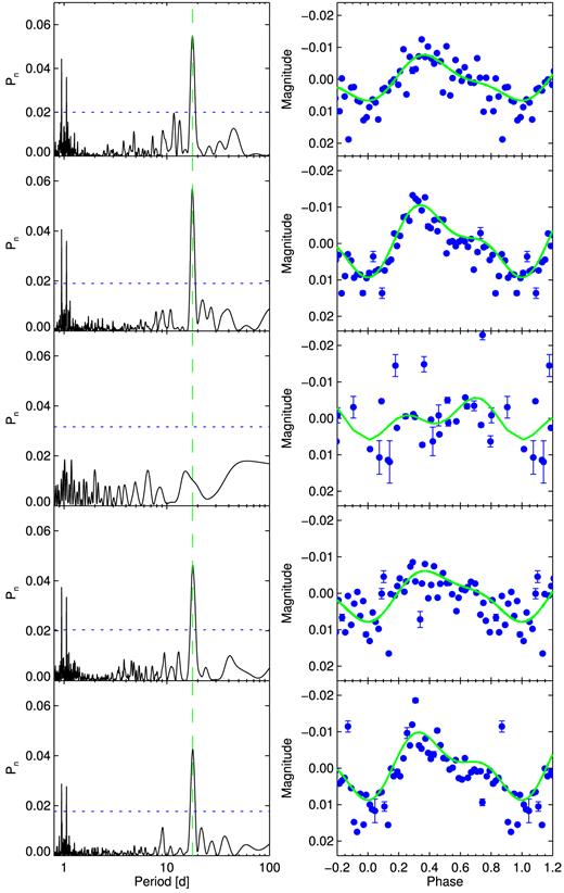
Left: Periodograms of the WASP light curves for WASP-164. Horizontal lines indicate false-alarm probability levels 0.1, 0.01, and 0.001. Right: Light curves phase-binned on the assumed rotation period of 17.81 d (points) with second-order harmonic series fit by least squares (lines). Data are plotted by season and camera in the same order top-to-bottom as in Table 7.
Periodogram analysis of the WASP light curves for WASP-164. Observing dates are JD-2450000, N is the number of observations used in the analysis, a is the semi-amplitude of the best-fitting sine wave at the period P found in the periodogram with false-alarm probability FAP.
| Camera | Dates | N | P [d] | a [mmag] | FAP |
|---|---|---|---|---|---|
| 221 | 5336-5515 | 7916 | 17.790 | 0.006 | <10−4 |
| 221 | 5699-5881 | 5623 | 17.730 | 0.007 | <10−4 |
| 221 | 6064-6106 | 1004 | 1.014 | 0.004 | 0.93 |
| 222 | 5352-5527 | 7906 | 17.850 | 0.006 | <10−4 |
| 222 | 5716-5897 | 5041 | 17.850 | 0.007 | <10−4 |
For WASP-147, WASP-160B, and WASP-165, a similar analysis leads to upper limits of 1.2 millimagnitudes, 2.9 millimagnitudes, and 1.2 millimagnitudes with 95 per cent confidence for the amplitude of any sinusoidal signal over the same frequency range, respectively.
3.3 Stellar evolution modelling
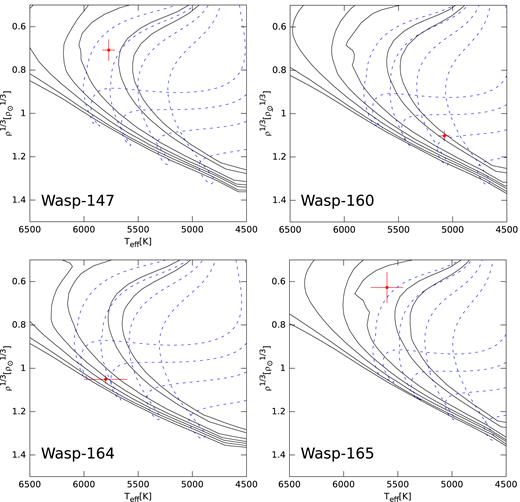
In order to estimate stellar parameters, we considered Teff, [Fe/H], log g, and |$v$|sin i inferred from spectral analysis (see Section 3.1), the mean stellar density ρ⋆ inferred from the transit light curve (see Section 4.1) and magnitude G, colour index GBP − GRP and distance d reported by Gaia DR2 (Gaia Collaboration et al. 2018). We analysed WASP-147 and WASP-160B using the set G, GBP − GRP, d, [Fe/H], log g, ρ⋆, and |$v$|sin i as input parameters. For WASP-164 and WASP-165, we adopted the same input set, but replaced the colour index by the spectroscopic temperature as it is more precisely known than that inferred from the Gaia colours. An extinction coefficient of Av = 0 was assumed in this analysis. We recovered the main stellar parameters such as age, mass, and radius according to theoretical models. We considered the grids of evolutionary tracks and isochrones computed by parsec2 (version 1.2S; see Bressan et al. (2012); Chen et al. (2014) and references therein).
The interpolation of the input data in the theoretical grids to retrieve the output parameters has been done according to the isochrone placement technique described in Bonfanti et al. (2015); Bonfanti, Ortolani & Nascimbeni (2016). Here we briefly recall that the algorithm makes a comparison between observations and theoretical isochrones and select those theoretical data which match the observations best. In particular, for each star
multiple grids of isochrones spanning the input metallicity range [[Fe/H]−Δ[Fe/H]; [Fe/H]+Δ[Fe/H]] have been loaded;
isochrones have been filtered through a two-dimensional Gaussian window function whose σ1 = ΔTeff, σ2 = Δlog L;
isochrones have been weighted evaluating the stellar evolutionary speed in the HR diagram and considering the similarity between theoretical and observational parameters;
the gyrochronological relation by Barnes (2010) has been used to set a conservative age lower limit to discard unlikely very young isochrones;
element diffusion has been taken into account.
Uncertainties given by the code are simply internal, i.e. they are related to the interpolation scheme in use. Realistic uncertainties to be attributed to stellar parameters should take also theoretical model uncertainties into account. By comparing the results with two independent evolutionary models (namely parsec and CLES, 3 Scuflaire et al. 2008), we find that systematics due to models can be estimated to be |${\sim }2{{\ \rm per\ cent}}$|. In addition, helium content Y influences theoretical models, but its quantity cannot be estimated from spectroscopy (at least in the case of solar-like stars). Given the uncertainty on Y, a further |${\sim }5{{\ \rm per\ cent}}$| should be added to the error budget. Fig. 8 shows the placement of the planet hosts in the HR diagram.
Placement of the planet host stars in the HR diagram. In each panel, theoretical models corresponding to the metallicity of that star are shown. Solid black lines are representative of isochrones: from left to right 0.5, 1, 2, 3.2, 5, 10, and 12.6 Gyr models are represented. Dashed blue lines are representative of evolutionary tracks: from left to right 1.1, 1, 0.9, and 0.8 M⊙ models are represented.
We also used the open source software bagemass4 to calculate the posterior mass distribution for each star using the Bayesian method described by Maxted, Serenelli & Southworth (2015). The models used in bagemass were calculated using the garstec stellar evolution code (Weiss & Schlattl 2008) using as input the spectroscopically derived Teff and [Fe/H] as well as the transit-derived ρ* and orbital Period. The mass and age of the stars found are shown in Table 8. They are in excellent agreement with the values derived above for WASP-147, 164, and 165. For WASP-160B, bagemass favours a slightly younger age and higher mass. This is due to the input selection of bagemass that includes the spectroscopically determined stellar effective temperature instead of the Gaia colour index.
Stellar mass and age estimates obtained with bagemass. The mean and standard deviation of the posterior distributions are given together with the best-fitting values in parentheses.
| Star | Mass [M⊙] | Age [Gyr] |
|---|---|---|
| WASP-147 | 1.08 ± 0.07 (1.05) | 8.4 ± 1.9 (9.1) |
| WASP-160B | 0.98 ± 0.04 (1.01) | 3.7 ± 2.3 (1.5) |
| WASP-164 | 0.96 ± 0.07 (1.02) | 4.7 ± 3.3 (2.0) |
| WASP-165 | 1.17 ± 0.09 (1.18) | 7.3 ± 2.2 (7.3) |
| Star | Mass [M⊙] | Age [Gyr] |
|---|---|---|
| WASP-147 | 1.08 ± 0.07 (1.05) | 8.4 ± 1.9 (9.1) |
| WASP-160B | 0.98 ± 0.04 (1.01) | 3.7 ± 2.3 (1.5) |
| WASP-164 | 0.96 ± 0.07 (1.02) | 4.7 ± 3.3 (2.0) |
| WASP-165 | 1.17 ± 0.09 (1.18) | 7.3 ± 2.2 (7.3) |
3.4 The WASP-160 binary
Due to the low resolution of the WASP instrument, photometry of WASP-160B was blended with a second, slightly brighter, source. While exploratory RV observations and transit follow-up quickly identified the origin of the transit the to be the fainter star, we found that both objects possess near-identical systemic RVs, pointing towards them being physically associated. This is confirmed by consistent Gaia proper motion and parallax values for both objects. To derive the properties of WASP-160A, we retrieved the stellar properties from a spectral analysis and stellar evolution models as described in Section 3.1 and 3.3. For the stellar evolution models, we used Gaia values for G, GBP − GRP, and d, and results from our spectroscopic analysis for [Fe/H], log g, and |$v$|sin i as inputs. As we have not detected any transiting planet around WASP-160A, no transit-derived value for ρ⋆ was available. Our handful of RV measurements of WASP-160A are stable within ∼40 |${\rm m\, s}^{-1}$|. We summarize the properties of WASP-160A and the WASP-160A + B binary in Table 9. Both stars appear to have similar masses and early K spectral types and their projected separation of 28.478948 ± 2.5 × 10⁻⁵ arcsec translates into a physical distance of 8060 ± 101 au. As WASP-160B, also WASP-160A has a super-Solar metallicity, ([Fe/H] = 0.19 ± 0.09), consistent within uncertainties with the value found for WASP-160B. Even though we would expect the two object to be coeval, we find a slightly older age for WASP-160A from evolutionary models. While this reinforces the older age estimate for WASP-160A, the discrepancy found in our analysis between objects A and B is likely an artefact of the very limited available data on WASP-160A.
Properties of WASP-160A and the WASP-160A + B binary.
| WASP-160A stellar properties | ||
|---|---|---|
| RA (J2000) | 05 50 44.7 | |
| DEC (J2000) | –27 37 05.0 | |
| UCAC4 B [mag] | 13.452 ± 0.04 | |
| UCAC4 V [mag] | 12.677 ± 0.02 | |
| 2MASS J [mag] | 11.300 ± 0.026 | |
| 2MASS H [mag] | 10.937 ± 0.024 | |
| 2MASS K [mag] | 10.831 ± 0.019 | |
| GAIA DR2 ID | 2910755484609594368 | |
| GAIA G [mag] | 12.5 | |
| GAIA GBP[mag] | 12.9 | |
| GAIA GRP[mag] | 11.9 | |
| Spectral Type | K0V | |
| Teff[K] | 5300 ± 150 | |
| log g[cgs] | 4.5 ± 0.2 | |
| [Fe/H] | 0.19 ± 0.09 | |
| Vrotsin i*[|${\rm km\, s}^{-1}$|]a | 0.4 ± 0.2 | |
| log A(Li) | – | |
| Mass [M|$\odot$|] | 0.89 ± 0.07 | |
| Radius [R|$\odot$| | 0.95 ± 0.07 | |
| Age [Gyr]b | 11.2 ± 1.6 | |
| Binary propertiesc | ||
| WASP-160A | WASP-160B | |
| Proper motion RA [mas] | 26.85 ± 0.03 | 26.97 ± 0.03 |
| Proper motion DEC [mas] | −34.82 ± 0.04 | −34.83 ± 0.04 |
| Parallax [mas] | 3.46 ± 0.03 | 3.44 ± 0.02 |
| Distance [pc]d | 282 ± 5 | 284 ± 5 |
| System RV [|${\rm km\, s}^{-1}$|] | −6.1587 ± 0.0075 | −6.1421 ± 0.0012 |
| Position angle of B with respect to A [deg] | −129.96 | |
| Separation [arcsec] | 28.478948 ± 2.5 × 10⁻⁵ | |
| Separation [au] | 8060 ± 101 | |
4 SYSTEM PARAMETERS
4.1 Modelling approach
We carried out a global analysis of all follow-up photometry and RVs for each planetary system using the Markov Chain Monte Carlo (MCMC) framework described by Gillon, M. et al. (2012). In short, our model consists of a Keplerian for the RVs and the prescription of Mandel & Agol (2002) for transit light curves. Next to the fitted (‘jump’) parameters listed in Table 10, the code allows for the inclusion of parametric baseline models in the form of polynomials (up to 4th order) when fitting transit light curves. We tested a wide range of baseline models, including dependencies on time, airmass, stellar FWHM, coordinate shifts and sky background, and finally selected the appropriate solution for each light curve via Bayes factor comparison (e.g. Schwarz 1978). The best baseline models are listed in Table 5. For all objects, we tested for a non-zero eccentricity by running two sets of global analyses: one while fixing the eccentricity to zero and one fitting for it by including |$\sqrt{e}\sin {\omega }$| and |$\sqrt{e}\cos {\omega }$| as jump parameters. We found no significant evidence for a non-circular orbit for any of our targets.
Planetary and stellar parameters from a global MCMC analysis.
| Parameter | WASP-147 | WASP-160B | WASP-164 | WASP-165 |
|---|---|---|---|---|
| Jump parameters | ||||
| Transit depth, ΔF | |$0.00640_{-0.00059}^{+0.00062}$| | |$0.01663_{-0.00038}^{+0.00043}$| | 0.01542 ± 0.00033 | |$0.00544_{-0.00059}^{+0.00067}$| |
| b′ = a*cos (ip) [R*] | |$0.31_{-0.21}^{+0.19}$| | |$0.20_{-0.12}^{+0.10}$| | |$0.8216_{-0.0091}^{+0.0084}$| | |$0.53_{-0.22}^{+0.11}$| |
| Transit duration, T14 [d] | |$0.1831_{-0.0033}^{+0.0041}$| | |$0.11851_{-0.00078}^{+0.00094}$| | |$0.06682_{-0.00084}^{+0.00085}$| | |$0.1740_{-0.0034}^{+0.0040}$| |
| Mid-transit time, [BJD] - 2450000 | 6562.5950 ± 0.0013 | 7383.65494 ± 0.00021 | 7203.85378 ± 0.00020 | 7649.71142 ± 0.00093 |
| Period, P [d] | 4.60273 ± 0.000027 | 3.7684952 ± 0.0000035 | 1.7771255 ± 0.0000028 | 3.465509 ± 0.000023 |
| |$K_2=K\sqrt{1-e^2}P^{1/3}$| [ms−1d1/3] | |$54.4_{-4.6}^{+4.7}$| | |$62.1_{-9.5}^{+9.2}$| | 445 ± 15 | 115 ± 16 |
| Stellar mass, M* [M|$\odot$|] | |$1.044_{-0.073}^{+0.070}$| | |$0.87_{-0.068}^{+0.071}$| | |$0.946_{-0.071}^{+0.067}$| | |$1.248_{-0.070}^{+0.072}$| |
| Stellar eff. temperature, Teff [K] | 5702 ± 100 | 5298 ± 99 | |$5806_{-200}^{+190}$| | 5599 ± 150 |
| Stellar metallicity, [Fe/H]* | |$0.092_{-0.071}^{+0.069}$| | 0.27 ± 0.10 | |$-0.01_{-0.20}^{+0.19}$| | 0.33 ± 0.13 |
| |$c_{1, \rm V}=2u_{1, \rm V}+u_{2, \rm V}$| | |$1.198_{-0.050}^{+0.051}$| | |||
| |$c_{2, \rm V}=u_{1, \rm V}-2u_{2, \rm V}$| | −0.014 ± 0.040 | |||
| |$c_{1, \rm R}=2u_{1, \rm R}+u_{2, \rm R}$| | |$1.042_{-0.082}^{+0.081}$| | |||
| |$c_{2, \rm R}=u_{1, \rm R}-2u_{2, \rm R}$| | |$-0.178_{-0.056}^{+0.053}$| | |||
| |$c_{1, \rm r^{\prime }}=2u_{1, \rm r^{\prime }}+u_{2, \rm r^{\prime }}$| | |$1.079_{-0.044}^{+0.046}$| | 1.200 ± 0.042 | |$1.022_{-0.074}^{+0.077}$| | |
| |$c_{2, \rm r^{\prime }}=u_{1, \rm r^{\prime }}-2u_{2, \rm r^{\prime }}$| | |$-0.133_{-0.032}^{+0.033}$| | 0.093 ± 0.036 | |$-0.178_{-0.059}^{+0.058}$| | |
| |$c_{1, \rm NGTS}=2u_{1, \rm NGTS}+u_{2, \rm NGTS}$| | 1.09 ± 0.10 | |||
| |$c_{2, \rm NGTS}=u_{1, \rm NGTS}-2u_{2, \rm NGTS}$| | 0.02 ± 0.11 | |||
| |$c_{1, \rm I+z^{\prime }}=2u_{1, \rm I+z^{\prime }}+u_{2, \rm I+z^{\prime }}$| | 0.94 ± 0.10 | 0.88 ± 0.10 | ||
| |$c_{2, \rm I+z^{\prime }}=u_{1, \rm I+z^{\prime }}-2u_{2, \rm I+z^{\prime }}$| | −0.07 ± 0.11 | |$-0.14_{-0.11}^{+0.10}$| | ||
| |$c_{1, \rm BB}=2u_{1, \rm BB}+u_{2, \rm BB}$| | 0.99 ± 0.10 | 0.99 ± 0.10 | ||
| |$c_{2, \rm BB}=u_{1, \rm BB}-2u_{2, \rm BB}$| | 0.00 ± 0.11 | −0.07 ± 0.11 | ||
| Deduced parameters | ||||
| RV amplitude, K [|${\rm m\, s}^{-1}$|] | 32.7 ± 2.8 | |$39.9_{-6.1}^{+5.9}$| | 367 ± 12 | 76 ± 10 |
| RV zero-point (pre-upgrade), γCOR1 [|${\rm km\, s}^{-1}$|] | −1.63849 ± 0.00061 | |||
| RV zero-point, γCOR2 [|${\rm km\, s}^{-1}$|] | |$-1.617011_{-0.000066}^{+0.000069}$| | −6.1421 ± 0.0012 | |$12.262676_{0.000091}^{+0.000094}$| | 25.6557 ± 0.0012 |
| Planetary radius, Rp [RJ] | |$1.115_{-0.093}^{+0.14}$| | |$1.090_{-0.041}^{+0.047}$| | |$1.128_{-0.043}^{+0.041}$| | |$1.26_{-0.17}^{+0.19}$| |
| Planetary mass, Mp [MJ] | |$0.275_{-0.027}^{+0.028}$| | |$0.278_{-0.045}^{+0.044}$| | |$2.13_{-0.13}^{+0.12}$| | |$0.658_{-0.092}^{+0.097}$| |
| Planetary mean density, ρp [ρJ] | |$0.198_{-0.060}^{+0.061}$| | |$0.214_{-0.038}^{+0.039}$| | |$1.48_{-0.13}^{+0.15}$| | |$0.33_{-0.11}^{+0.19}$| |
| Planetary grav. acceleration, |${\log g}_{p}$| [cgs] | |$2.74_{-0.11}^{+0.08}$| | |$2.763_{-0.077}^{+0.066}$| | |$3.619_{-0.028}^{+0.029}$| | |$3.01_{-0.13}^{+0.14}$| |
| Planetary eq. temperature, Teq [K]a | |$1404_{-43}^{+69}$| | |$1119_{-23}^{+25}$| | |$1610_{-53}^{+58}$| | |$1624_{-89}^{+93}$| |
| Orbital semimajor axis, a [au] | |$0.0549_{-0.0013}^{+0.0012}$| | 0.0452 ± 0.0012 | |$0.02818_{-0.00072}^{+0.00065}$| | |$0.04823_{-0.00092}^{+0.00091}$| |
| a/R* | |$8.29_{-0.74}^{+0.40}$| | |$11.25_{-0.31}^{+0.19}$| | 6.50 ± 0.13 | |$5.93_{-0.55}^{+0.67}$| |
| Rp/R* | 0.0800 ± 0.0038 | |$0.1290_{-0.0015}^{+0.0017}$| | 0.1242 ± 0.0013 | |$0.0738_{-0.0041}^{+0.0044}$| |
| Inclination, ip [deg] | |$87.9_{-1.6}^{+1.5}$| | |$88.97_{-0.57}^{+0.63}$| | |$82.73_{-0.21}^{+0.22}$| | |$84.9_{-1.7}^{+2.5}$| |
| Eccentricity, e | 0 (<0.19 at 1σ) | 0 (<0.22 at 1σ) | 0 (<0.09 at 1σ) | 0 (<0.14 at 1σ) |
| Stellar radius, R* [R|$\odot$|] | |$1.429_{-0.076}^{+0.14}$| | |$0.868_{-0.028}^{+0.031}$| | |$0.932_{-0.030}^{+0.028}$| | 1.75 ± 0.18 |
| Stellar mean density, ρ* [ρ|$\odot$|] | |$0.361_{-0.088}^{+0.054}$| | |$1.34 _{-0.11}^{+0.07}$| | |$1.165_{-0.067}^{+0.074}$| | |$0.233_{-0.059}^{+0.089}$| |
| Limb-darkening coefficient, |$u_{1, \rm V}$| | 0.477 ± 0.027 | |||
| Limb-darkening coefficient, |$u_{2, \rm V}$| | 0.245 ± 0.018 | |||
| Limb-darkening coefficient, |$u_{1, \rm R}$| | 0.381 ± 0.040 | |||
| Limb-darkening coefficient, |$u_{2, \rm R}$| | |$0.280_{-0.020}^{+0.021}$| | |||
| Limb-darkening coefficient, |$u_{1, \rm r^{\prime }}$| | |$0.405_{-0.023}^{+0.024}$| | 0.499 ± 0.022 | 0.373 ± 0.038 | |
| Limb-darkening coefficient, |$u_{2, \rm r^{\prime }}$| | 0.269 ± 0.015 | 0.203 ± 0.017 | |$0.276_{-0.023}^{+0.022}$| | |
| Limb-darkening coefficient, |$u_{1, \rm NGTS}$| | 0.440 ± 0.056 | |||
| Limb-darkening coefficient, |$u_{2, \rm NGTS}$| | 0.210 ± 0.058 | |||
| Limb-darkening coefficient, |$u_{1, \rm I+z^{\prime }}$| | 0.363 ± 0.053 | |$0.323_{-0.047}^{+0.048}$| | ||
| Limb-darkening coefficient, |$u_{2, \rm I+z^{\prime }}$| | 0.215 ± 0.056 | |$0.232_{-0.047}^{+0.049}$| | ||
| Limb-darkening coefficient, |$u_{1, \rm BB}$| | 0.398 ± 0.053 | |$0.384_{-0.048}^{+0.047}$| | ||
| Limb-darkening coefficient, |$u_{2, \rm BB}$| | 0.196 ± 0.055 | |$0.224_{-0.048}^{+0.051}$| | ||
Note: aEquilibrium temperature, assuming AB = 0 and F = 1 (Seager et al. 2005).
To estimate excess noise, we calculated the |$\beta _{\mathit {r}}$| and |$\beta _{\mathit {w}}$| (Winn et al. 2008; Gillon et al. 2010) factors that compare the rms of the binned and unbinned residuals and multiplied our error bars by their product before deriving the final parameter values. We find no excess ‘jitter’ noise in the RVs and thus do not adapt the RV errors. We adopted a quadratic stellar limb-darkening law using coefficients interpolated from the tables by Claret & Bloemen (2011). To use the most appropriate input stellar parameters, we use the information extracted from the stellar spectra, paired with the Gaia DR2 (Gaia Collaboration et al. 2018) data as described in Section 3. After carrying out an initial analysis to measure transit-based stellar mean densities needed to constrain the evolutionary models, we placed normal priors on M*, [Fe/H]*, and Teff centred on the values inferred in Section 3, with a width of the quoted 1 − σ uncertainties. The four objects under study are revealed to be gas giants, two of them being classical hot Jupiters, while two have masses near that of Saturn.
4.2 WASP-147
WASP-147b is a Saturn-mass (M = 0.27MJ) planet orbiting a G4 star with a period of 4.6 d. The system appears to be old, with the 1.04 M|$\odot$| host having started to evolve off the main sequence. Stellar evolutionary modeling places the star’s age at 8.5 ± 0.8 Gyr, and its old age is corroborated by a low Lithium abundance that is in accordance with measurements for stars aged 2 Gyr or more (Sestito & Randich 2005) and the absence of activity indicators such as excess RV stellar noise and rotational variability. The planet is one of the more strongly irradiated planets of its mass range. Considering the mass-incident flux plane shown in Fig. 9, WASP-147b is located near the inner tip of the triangular sub-Saturn desert (Mazeh, Zucker & Pont 2005; Szabó & Kiss 2011; Mazeh, Holczer & Faigler 2016), which appears to be created by erosion of planetary atmospheres due to stellar irradiation (Lammer et al. 2003; Baraffe et al. 2006). Being a low-mass, low-density planet, WASP-147b is a good target for transmission spectroscopy. One atmospheric scale height translates to a predicted change in the transit depth of 249 ppm, well within the precision of ground- and space-based transmission spectra (e.g. Kreidberg et al. 2015; Sing et al. 2016; Lendl et al. 2017; Sedaghati et al. 2017).
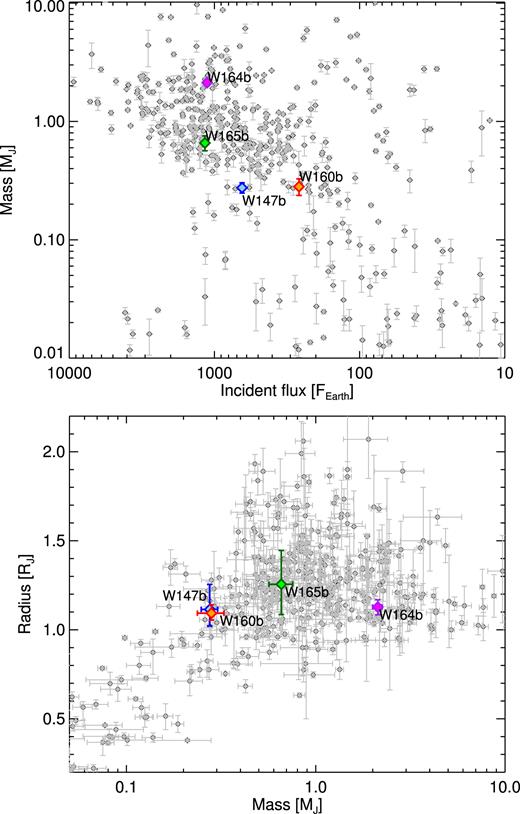
Top: Planetary masses against incident flux for known exoplanets. Only planets with well-measured masses and radii (relative uncertainties smaller than 50 per cent) are shown. Our newly discovered objects are shown in colour and labelled. Bottom: Planetary mass-radius diagram. Sample selection and designation of our targets as above.
4.3 WASP-160B
Similar to WASP-147b, WASP-160Bb is also a near Saturn-mass (Mp = 0.28 MJ) object, however this planet orbits a cooler K0V star in a wide (28.5 arcsec) near equal-mass binary with a period of 3.8 d. The stellar age is estimated to be approximately 10 Gyr from evolutionary models, and a non-detection of Lithium supports the object’s old age. In contrast to WASP-147, the later-type WASP-160B still resides firmly on the main sequence. Both planets share near-identical mass and radius, however WASP-160Bb orbits a very metal-rich star (|$\mathbf {\mathrm{[Fe/H]=0.27\pm 0.1}}$|), while WASP-147’s metallicity is near-Solar. WASP-160Bb receives less stellar irradiation than the bulk of hot Jupiters (see Fig. 9), which translates to a moderate equilibrium temperature of approx. 1100 K. Prospects for studying this object’s atmospheric transmission spectrum are excellent, as one atmospheric scale height translates to a radius variation of 338 ppm. To date, the only hot Jupiter orbiting a more metal-rich host with a characterized transmission spectrum is XO-2 (Burke et al. 2007; Sing et al. 2011), for which both Na and K have been detected.
4.4 WASP-164
WASP-164b is a massive (Mp = 2.13MJ) planet on a close-in orbit around a G2V star. Owing to the limited S/N of the follow-up spectra obtained, the stellar properties are somewhat more uncertain than for the other objects presented here. However, rotational modulation with a period of 17.81 ± 0.03 d seen in the survey light curve indicates a relatively young age of |$2.3_{-0.5}^{+1}$| Gyr and evolutionary models confirm the star being located on the main sequence. The planet is rather massive compared to the bulk of hot Jupiters and orbits its host star with a short orbital period of 1.78 d at a separation of 2.74 times its Roche limit. This is consistent with expectations from high-eccentricity migration mechanisms (Ford & Rasio 2006). Being rather massive and close-in, the planet may be further undergoing orbital decay through tidal dissipation (e.g. Rasio et al. 1996; Levrard, Winisdoerffer & Chabrier 2009; Matsumura, Peale & Rasio 2010). Using a value of |$\log {Q^{\prime }_{s}}=8.26\pm 0.14$| (Collier Cameron & Jardine 2018), we find a remaining lifetime of 13.0 ± 4.6 Gyr. The planetary orbit is thus not expected to shrink drastically due to tidal dissipation over the star’s main-sequence lifetime. The planet’s close-in orbital period is however advantageous for the object’s atmospheric characterization. Indeed, WASP-164b makes for a promising target for characterization via emission spectroscopy, with a predicted occultation depth in H band between 450 ppm (full redistribution) and 1125 ppm (immediate reradiation).
4.5 WASP-165
WASP-165b is a classical hot Jupiter. With an orbital period of 3.4 d, it lies near the peak of the hot Jupiter period distribution while its mass (MP = 0.66MJ) and radius (RP = 1.26RJ) are typical for this class of planet (see Fig. 9). With respect to planetary mass, radius, and period, WASP-165b is near-identical to the extremely well-studied object HD 209458b (Charbonneau et al. 2000; Henry et al. 2000; Mazeh et al. 2000), however WASP-165b is more strongly irradiated as its |$M_\ast =1.25 \,{{\rm M}_{\odot }}$| G6 host has started evolving off the main sequence. The system’s age estimate from evolutionary models is 4.8 ± 1 Gyr, albeit the object’s Lithium abundance suggests a slightly younger age of 0.5–2 Gyr. This discrepancy is most likely due to the limited S/N of our spectra. We consider the age estimate from evolutionary models as more accurate, as these contain the stellar mean density inferred from the high-precision follow-up light curves. As WASP-160B, also WASP-165 has a remarkably high metallicity of [Fe/H] = 0.33 ± 0.13.
5 SUMMARY
We present the discovery of four transiting hot Jupiters by WASP-South. WASP-147b and WASP-160Bb are Saturn-mass planets with near-identical radii but contrasting stellar metallicities and planetary equilibrium temperatures: the 1400 K WASP-147b orbits a Solar-metallicity G4 star, while the 1100 K WASP-160Bb orbits a metal-rich K0 star in a near equal-mass binary. Both objects are promising targets for atmospheric characterization via transmission spectroscopy. WASP-164b is a massive (|$2.1\, {{M}_{J}}$|) planet on a short (1.8 d) orbital period, and a potential target for emission spectroscopy. Finally, WASP-165b is a classical hot Jupiter orbiting a metal-rich host.
SUPPORTING INFORMATION
Table 1. RV measurements of WASP-147.
Table 2. RV measurements of WASP-160B.
Table 3. RV measurements of WASP-164.
Table 4. RV measurements of WASP-165.
Please note: Oxford University Press is not responsible for the content or functionality of any supporting materials supplied by the authors. Any queries (other than missing material) should be directed to the corresponding author for the article.
ACKNOWLEDGEMENTS
WASP-South is hosted by the South African Astronomical Observatory and we are grateful for their ongoing support and assistance. Funding for WASP comes from consortium universities and from the UK’s Science and Technology Facilities Council. TRAPPIST is funded by the Belgian Fund for Scientific Research (Fond National de la Recherche Scientifique, FNRS) under the grant FRFC 2.5.594.09.F, with the participation of the Swiss National Science Fundation (SNF). MG is a F.R.S.-FNRS Senior Research Associate. The research leading to these results has received funding from the European Research Council under the FP/2007-2013 ERC Grant Agreement 336480, from the ARC grant for Concerted Research Actions financed by the Wallonia-Brussels Federation, and from the Balzan Foundation. LD acknowledges support from the Gruber Foundation Fellowship. ML acknowledges support from the Austrian Research Promotion Agency (FFG) under project 859724 ‘GRAPPA’.
Footnotes
According to exoplanets.eu, queried on 2018 April 12.
Padova and Trieste Stellar Evolutionary Code. http://stev.oapd.inaf.it/cgi-bin/cmd
Code Liégeois d’Evolution Stellaire
