


ABSTRACT
We constrain the mass–richness scaling relation of redMaPPer galaxy clusters identified in the Dark Energy Survey Year 1 data using weak gravitational lensing. We split clusters into 4 × 3 bins of richness λ and redshift |$z$| for λ ≥ 20 and 0.2 ≤ |$z$| ≤ 0.65 and measure the mean masses of these bins using their stacked weak lensing signal. By modelling the scaling relation as 〈M200m|λ, |$z$|〉 = M0(λ/40)F((1 + |$z$|)/1.35)G, we constrain the normalization of the scaling relation at the 5.0 per cent level, finding M0 = [3.081 ± 0.075(stat) ± 0.133(sys)] · 1014 M⊙ at λ = 40 and |$z$| = 0.35. The recovered richness scaling index is F = 1.356 ± 0.051 (stat) ± 0.008 (sys) and the redshift scaling index G = −0.30 ± 0.30 (stat) ± 0.06 (sys). These are the tightest measurements of the normalization and richness scaling index made to date from a weak lensing experiment. We use a semi-analytic covariance matrix to characterize the statistical errors in the recovered weak lensing profiles. Our analysis accounts for the following sources of systematic error: shear and photometric redshift errors, cluster miscentring, cluster member dilution of the source sample, systematic uncertainties in the modelling of the halo–mass correlation function, halo triaxiality, and projection effects. We discuss prospects for reducing our systematic error budget, which dominates the uncertainty on M0. Our result is in excellent agreement with, but has significantly smaller uncertainties than, previous measurements in the literature, and augurs well for the power of the DES cluster survey as a tool for precision cosmology and upcoming galaxy surveys such as LSST, Euclid, and WFIRST.
1 INTRODUCTION
Galaxy clusters have the potential to be the most powerful cosmological probe (Dodelson et al. 2016). Current constraints are dominated by uncertainties in the calibration of cluster masses (e.g. Rozo et al. 2010; Mantz et al. 2015a; Planck Collaboration XXIV 2016). Weak lensing allows us to determine the mass of galaxy clusters: gravitational lensing of background galaxies by foreground clusters induces a tangential alignment of the background galaxies around the foreground cluster. This alignment is a clear observational signature predicted from clean, well-understood physics. Moreover, the resulting signal is explicitly sensitive to all of the cluster mass, not just its baryonic component, and is insensitive to the dynamical state of the cluster. For all these reasons, weak lensing is the most robust method currently available for calibrating cluster masses. It is therefore not surprising that the community has invested in a broad range of weak lensing experiments specifically designed to calibrate the masses of galaxy clusters (Applegate et al. 2014; von der Linden et al. 2014a,b; Hoekstra et al. 2015; Mantz et al. 2015b; Okabe & Smith 2016; Dietrich et al. 2017; Melchior et al. 2017; Simet et al. 2017; Medezinski et al. 2018b; Miyatake et al. 2018; Murata et al. 2018).
The Dark Energy Survey (DES) is a 5000 square degree photometric survey of the southern sky. It uses the 4-m Blanco Telescope and the Dark Energy Camera (Flaugher et al. 2015) located at the Cerro Tololo Inter-American Observatory. As its name suggests, the primary goal of the DES is to probe the physical nature of dark energy, in addition to constraining the properties and distribution of dark matter. Owing to its large area, depth, and image quality, at its conclusion DES will support optical identification of |${\sim }100\, 000$| galaxy clusters and groups up to redshift |$z$| ≈ 1. We use galaxy clusters identified using the redMaPPer algorithm (Rykoff et al. 2014), which assigns each cluster a photometric redshift and optical richness λ of red galaxies. To fully utilize these clusters, one must understand mass-observable relations (MORs), such as that between cluster mass and optical richness. Weak lensing can establish this relation – with high statistical uncertainty for individual clusters, but low systematic uncertainty in the mean mass scale derived from the joint signal of large samples.
In this work, we use stacked weak lensing to measure the mean galaxy cluster mass of redMaPPer galaxy clusters identified in DES Year 1 (Y1) data. We use these data to calibrate the mass–richness–redshift relation of these clusters. In Melchior et al. (2017), we provided a first calibration of this relation using DES Science Verification (SV) data. There, we were able to achieve a 9.2 per cent statistical and 5.1 per cent systematic uncertainty. Here, we update that result using the first year of regular DES observations, incorporating a variety of improvements to the analysis pipeline. Our results provide the tightest, most accurate calibration of the richness–mass relation of galaxy clusters to date, at 2.4 per cent statistical and 4.3 per cent systematic uncertainty.
The structure of this paper is as follows. In Section 2, we introduce the DES Y1 data used in this work. In Section 3, we describe our methodology for obtaining ensemble cluster density profiles from stacked weak lensing shear measurements, with a focus on updates relative to Melchior et al. (2017). A comprehensive set of tests and corrections for systematic effects is presented in Section 4. The model of the lensing data and the inferred stacked cluster masses are given in Section 5. The main result, the mass–richness–redshift relation of redMaPPer clusters in DES, is presented in Section 6. We compare our results to other published works in the literature in Section 7, discuss systematic improvements made in this work compared to Melchior et al. (2017) in Section 8, and conclude in Section 9. In Appendix A, we present the DES Y1 redMaPPer catalogue used in this work for public use. Supplementary information on the analysis is given in additional appendices.
Unless otherwise stated, we assume a flat ΛCDM cosmology with Ωm = 0.3 and H0 = 70 km s−1 Mpc−1, with distances defined in physical coordinates, rather than comoving. Finally, unless otherwise noted all cluster masses refer to |$M_{200\rm {m}}$|. That is, cluster mass is defined as the mass enclosed within a sphere whose average density is 200 times higher than the mean cosmic matter density |$\bar{\rho }_m$| at the cluster’s redshift, matching the mass definition used in the cosmological analyses that make use of our calibration.
2 THE DES YEAR 1 DATA
DES started its main survey operations in 2013, with the Year One (Y1) observational season running from August 31, 2013 to February 9, 2014 (Drlica-Wagner et al. 2018). During this period, 1839 deg2 of the southern sky were observed in three to four tilings in each of the four DES bands g, r, i, |$z$|, as well as ∼1800 deg2 in the Y-band. The resulting imaging is shallower than the SV data release but covers a significantly larger area. In this study, we utilize approximately 1500 deg2 of the main survey, split into two large non-contiguous areas. This is a reduction from the 1800 deg2 area due to a series of veto masks. These masks include masks for bright stars and the Large Magellanic Cloud, among others. The two non-contiguous areas are the ‘SPT’ area (1321 deg2), which overlaps the footprint of the South Pole Telescope Sunyaev-Zel’dovich Survey (Carlstrom et al. 2011), and the ‘S82’ area (116 deg2), which overlaps the Stripe-82 deep field of the Sloan Digital Sky Survey (SDSS; Annis et al. 2014). The DES Y1 footprint is shown in Fig. 1.
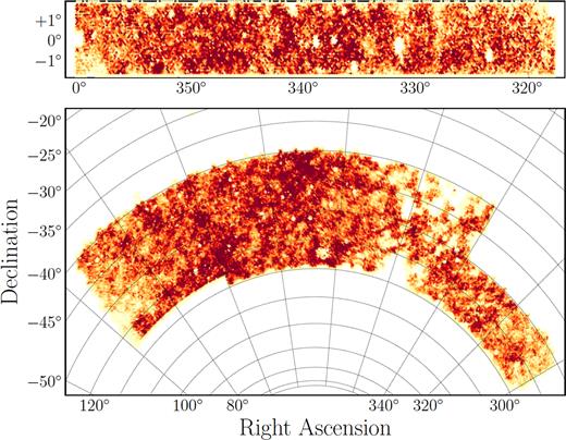
Surface density of source galaxies in the metacalibration catalogue within the DES Y1 footprint in the ‘S82’ field (top) and the ‘SPT’ field (bottom).
In the following, we briefly describe the main data products used in this analysis, and refer the reader to the corresponding papers for more details. The input photometric catalog, as well as the photometric redshift and weak lensing shape catalogues used in this study have already been employed in the cosmological analysis combining galaxy clustering and weak lensing by the DES collaboration (DES Collaboration et al. 2018).
2.1 Photometric catalogue
Input photometry for the redMaPPer cluster finder (Section 2.2) and photometric redshifts (Section 2.4) were derived from the DES Y1A1 Gold catalogue (Drlica-Wagner et al. 2018). Y1A1 Gold is the science–quality internal photometric catalogue of DES created to enable cosmological analyses. This data set includes a catalogue of objects as well as maps of survey depth and foreground masks, and star–galaxy classification. In this work, we make use of the multi-epoch, multi-object fitting (MOF) composite model (CM) galaxy photometry. The MOF photometry simultaneously fits a point spread function (psf)-convolved galaxy model to all available epochs and bands for each object, while subtracting and masking neighbours. The typical 10σ limiting magnitude inside 2″ diameter apertures for galaxies in Y1A1 Gold using MOF CM photometry is g ≈ 23.7, r ≈ 23.5, i ≈ 22.9, and |$z$| ≈ 22.2. Due to its low depth and calibration uncertainty, we do not use Y-band photometry for shape measurement or photometric redshift estimation.
The galaxy catalogue used for the redMaPPer cluster finder is constructed as follows. Bad objects that are determined to be catalogue artefacts, including having unphysical colours, astrometric discrepancies, and PSF model failures are rejected (Section 7.4 Drlica-Wagner et al. 2018). Galaxies are then selected via the more complete MODEST_CLASS classifier (Section 8.1 Drlica-Wagner et al. 2018). Only galaxies that are brighter in |$z$| band than the local |$10\, \sigma$| limiting magnitude are used by redMaPPer. The average survey limiting magnitude is deep enough to image a 0.2 L* galaxy at |$z$| ≈ 0.7. Finally, we remove galaxies in regions that are contaminated by bright stars, bright nearby galaxies, globular clusters, and the Large Magellanic Cloud.
2.2 Cluster catalog
We use a volume-limited sample of galaxy clusters detected in the DES Y1 photometric data using the redMaPPer cluster finding algorithm v6.4.17 (Rykoff et al. 2014, 2016). This redMaPPer version is fundamentally the same as the v6.3 algorithm described in Rykoff et al. (2016), with minor updates.
Two versions of the redMaPPer cluster catalog are generated: a ‘flux limited’ version, which includes high-redshift clusters for which the richness requires extrapolation along the cluster luminosity function, and one that is locally volume-limited. By ‘locally volume-limited’ we mean that at each point in the sky, a galaxy cluster is included in the sample if and only if all cluster galaxies brighter than the luminosity threshold used to define cluster richness in redMaPPer lie above |$10\, \sigma$| in |$z$|, |$5\, \sigma$| in i and r, and |$3\, \sigma$| in g according to the survey MOF depth maps (Drlica-Wagner et al. 2018). That is, no extrapolation in luminosity is required when estimating cluster richness. At the threshold, the galaxy sample is >90–95 per cent complete. It is this volume-limited cluster sample that is used in follow-up work deriving cosmological constraints from the abundance of galaxy clusters. Consequently, we focus exclusively on this volume-limited sample in this work. It contains more than 76 000 clusters down to λ > 5, of which more than 6500 are above λ = 20. The format of the catalogues are described in Appendix A.
redMaPPer identifies galaxy clusters as overdensities of red-sequence galaxies. Starting from an initial set of spectroscopic seed galaxies, the algorithm iteratively fits a model for the local red-sequence, and finds cluster candidates while assigning a membership probability to each potential member. Clusters are centred on bright galaxies selected using an iteratively self-trained matched-filter method. The method allows for the inherent ambiguity of selecting a central galaxy by assigning a probability to each galaxy of being the central galaxy of the cluster. The final membership probabilities of all galaxies in the field are assigned based on spatial, colour, and magnitude filters.
The distribution of cluster richness and redshift of the DES volume-limited cluster sample is shown in Fig. 2. The richness estimate λ is the sum over the membership probabilities of all galaxies within a pre-defined, richness–dependent projected radius Rλ. The radius Rλ is related to the cluster richness via Rλ = 1.0(λ/100)0.2 h−1Mpc. This relation was found to minimize the scatter between richness and X-ray luminosity in Rykoff et al. (2012). A redshift estimate for each cluster is obtained by maximizing the probability that the observed colour-distribution of likely members matches the self-calibrated red-sequence model of redMaPPer.
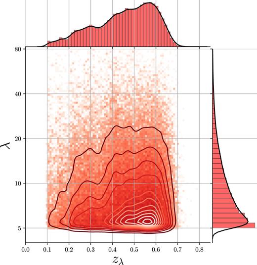
Redshift–richness distribution of redMaPPer clusters in the volume-limited DES Y1 cluster catalogue, overlaid with density contours to highlight the densest regions. At the top and on the right are histograms of the projected quantities, |$z$|λ and λ, respectively, with smooth kernel density estimates overlaid.
Fig. 3 shows the photometric redshift performance of the DES Y1 volume-limited redMaPPer cluster sample. The photometric redshift bias and scatter are calculated by comparing the photometric redshift of the clusters to the spectroscopic redshift of the central galaxy of the cluster, where available. Unfortunately, the small overlap with existing spectroscopic surveys means that our results are limited by small-number statistics: there are only 333 galaxy clusters with a spectroscopic central galaxy, and only 34 (six) with redshift |$z$| ≥ 0.6 (|$z$| ≥ 0.65). Nevertheless, the photometric redshift performance is consistent with our expectations: our redshifts are very nearly unbiased, and have a remarkably tight scatter — the median value of σ|$z$|/(1 + |$z$|) is ≈0.006. An upper limit for the photometric redshift bias of 0.003 is consistent with our data.
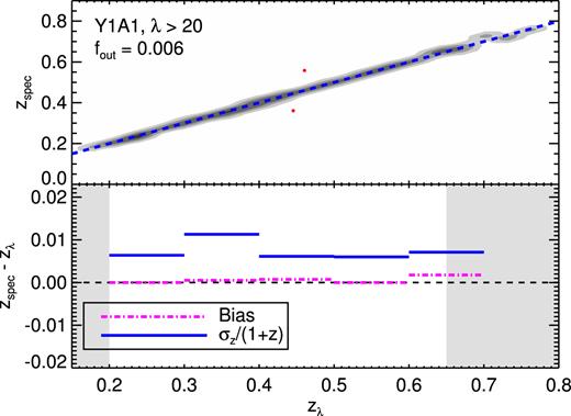
Photometric redshift performance of the DES Y1 redMaPPer cluster catalogue, as evaluated using available spectroscopy (333 clusters). Upper panel: Gray con tours are 3σ confidence intervals, and the two red dots are the only 4σ outliers, caused by miscentring on a foreground/background galaxy. Lower Panel: photo-|$z$| bias and uncertainty. The comparatively large uncertainty from 0.3 < |$z$| < 0.4 is due to a filter transition.
Of particular importance to this work is the distribution of miscentred clusters – both the frequency and severity of their miscentring. Based on the redMaPPer centring probabilities, we would expect ≈80 per cent of the clusters to be correctly centred, meaning the most likely redMaPPer central galaxy is at the centre of the potential well of the host halo. In practice, the fraction of correctly centred galaxy clusters is closer to ≈70 per cent, as estimated from a detailed comparison of the redMaPPer photometric centres to the X-ray centres of redMaPPer clusters for which high-resolution X-ray data is available (von der Linden et al., in preparation; Zhang et al., in preparation). The expected impact of this miscentring effect, and the detailed model for the miscentred distribution from Zhang et al. (in preparation) and von der Linden et al. (in preparation) is described in Section 5.2.
2.3 Shear catalogs
Our work uses the DES Y1 weak lensing galaxy shape catalogues presented in Zuntz et al. (2018). Two independent catalogues were created: metacalibration (Sheldon & Huff 2017; Huff & Mandelbaum 2017) based on ngmix (Sheldon 2015), and im3shape (Zuntz et al. 2013). Both pass a multitude of tests for systematics, making them suitable for cosmological analyses. While the Y1 data is shallower than the DES SV data, improvements in the shear estimation pipelines and overall data quality enabled us to reach a number density of sources similar to that from DES SV data (Jarvis et al. 2016).
In this study, we will focus exclusively on the metacalibration shear catalogue because of its larger effective source density (6.28 arcmin−2) compared to the im3shape catalogue (3.71 arcmin−2). The difference mainly arises because metacalibration utilizes images taken in r, i, |$z$| bands, whereas im3shape relies exclusively on r-band data. In the metacalibration shear catalogue, the fiducial shear estimates are obtained from a single Gaussian fit via the ngmix algorithm. As a supplementary data product, metacalibration provides (g, r, i, |$z$|)-band fluxes and the corresponding error estimates for objects using its internal model of the galaxies.
Galaxy shape estimators, such as the ngmix model-fitting procedure used for metacalibration, are subject to various sources of systematic errors. For a stacked shear analysis, the dominant problem is a multiplicative bias, i.e. an over- or underestimation of gravitational shear as inferred from the mean tangential ellipticity of lensed galaxies. This bias needs to be characterized and corrected. Traditionally, this is done using simulated galaxy images – with the critical limitation that simulations never fully resemble the observations.
|$\mathsf {R}$| is a 2 × 2 Jacobian matrix for the two ellipticity components e1, e2 in a celestial coordinate system. For the metacalibration mean shear measurements in this work, we calculate the response of mean tangential shear on mean tangential ellipticity. |$\mathsf {R}$| is close to isotropic on average, which is why other recent weak lensing analyses (Prat et al. 2018; Troxel et al. 2018; Chang et al. 2018; Gruen et al. 2018) have assumed it to be a scalar. For the larger tangential shears measured on small scales around clusters, however, we account for the fact that the response might not be quite isotropic by explicitly rotating it to the tangential frame.
Blinding procedure
As a precaution against unintentional confirmation bias in the scientific analyses, both weak lensing shape catalogues produced for DES Y1 had an unknown blinding factor in the magnitude of |$\mathbf {e}$| (Zuntz et al. 2018) applied to them. This unknown factor was constrained between 0.9 and 1.1. While we made initial blinded measurements for this work, the factor was revealed as part of unblinding the cosmology results of DES Collaboration et al. (2018).
In accordance with the practices of other DES Y1 cosmology analyses, we have further adopted a secondary layer of blinding. Specifically, we blindly transform the chains from our MCMCs to hide our in-progress results, and to prevent comparison between our cluster masses and those estimated using mass–observable relations from the literature. Chains of the parameters in the modelled lensing profiles and the mass–richness relation were unaltered after unblinding.
2.4 Photometric redshift catalogue
In interpreting the weak gravitational lensing signal of galaxy clusters as physical mass profiles, we need to employ information about the geometry of the source–lens systems by considering the relevant angular–diameter distances. To calculate these distances, we rely on estimates of the overall redshift distribution of source galaxies, and also on information about the individual P(|$z$|) of source galaxies.
We use the DES Y1 photometric redshifts estimated and validated by Hoyle et al. (2018) using the template-based bpz algorithm (Benítez 2000; Coe et al. 2006). It was found by Hoyle et al. (2018) that these photo-z estimates were modestly biased, introducing an overall multiplicative systematic correction in the recovered weak lensing profiles. We determine this correction and its systematic uncertainty in Section 4.3.
In order to be able to correct selection effects due to the change of photo-|$z$| with shear while utilizing the highest signal-to-noise flux measurements for determining the source redshift distribution, we use two separate BPZ catalogues: one generated from metacalibration-measured photometry (for selecting and weighting sources), and one from MOF (see Section 2.1) photometry (for determining the resulting source redshift distributions). Details of this are described in the following section.
3 STACKED LENSING MEASUREMENTS
3.1 Mass density profiles
3.1.1 The lensing estimator
Due to the low signal-to-noise of individual source–lens pairs, we measure the stacked (mean) signal of many source galaxies around a selection of clusters.
3.1.2 Practical lensing estimator
The use of two different photometric estimators is necessary because when calculating the selection response, the internal photometry of the metacalibration, with measurements on sheared images, must be used for all selection and weighting of sources. Hoyle et al. (2018) find this photometric redshift estimate to have a greater scatter than the default MOF photometry. We therefore opt to use the metacalibration photo-|$z$| estimates only for selecting and weighting source–lens pairs. When normalizing the shear signal to find ΔΣ, we utilize the MOF-based photo-|$z$| estimates.
3.1.3 Data vector binned in redshift and richness
In estimating the lensing signal through equation (12), we utilize a modified version of the publicly available xshear code1 and the custom-built xpipe python package.2 The core implementation of the measurement code is identical to the one used by Melchior et al. (2017).
We group the clusters into three bins in redshift: |$z$| ∈ [0.2; 0.4), [0.4; 0.5), and [0.5; 0.65), as well as seven bins in richness: λ ∈ [5; 10), [10; 14), [14; 20), [20; 30), [30; 45), [45; 60), and [60; ∞). The redshift limit |$z$| = 0.65 of our highest redshift corresponds roughly to the highest redshift for which the redMaPPer cluster catalogue remains volume-limited across the full DES Y1 survey footprint. The ΔΣ profiles were measured in 15 logarithmically spaced radial bins ranging from 0.03 Mpc to 30 Mpc. For our later results, we will only utilize the radial range above 200 kpc. Scales below this cut are included only in our figures and for reference purposes, and are excluded from the analysis to avoid systematic effects such as obscuration, significant membership contamination, and blending. This radial binning scheme yields similar S/N across all bins. The measured shear profiles are shown in Fig. 4.
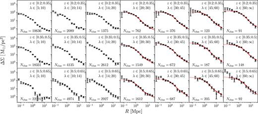
Mean ΔΣ for cluster subsets split in redshift |$z$|l (increasing from top to bottom) and λ (increasing from left to right), as labelled. The error bars shown are the diagonal entries of our semi-analytic covariance matrix estimate (see Section 3.2) for bins with λ > 20 and the jackknife-estimated covariance matrix for bins with λ < 20. The best-fit model (red curve) is shown for bins with λ > 20, and includes dilution from cluster member galaxies (Section 5.3.1) and miscentring (Section 5.2); see Section 5 for details. Semi-analytic covariances were not computed for stacks with λ < 20 due to the significant computational cost. Below 200 kpc, we consider data points unreliable and therefore exclude them from our analysis; these are indicated by open symbols and dashed lines. The profiles and jackknife errors are calculated after the subtraction of the random-point shear signal (see Section 4.1.3).
We find a mild radial dependence in the typical value for metacalibration shear response |$\langle \mathsf {R}_{\gamma , \mathrm{T}} \rangle$|, the asymptotic values are 0.6, 0.58, and 0.55 as a function of increasing cluster redshift. For the selection response, we find an asymptotic value of |$\langle \mathsf {R}_{\rm sel} \rangle \approx$| 0.013, 0.014, and 0.015.
3.2 Covariance matrices
The ΔΣ profiles estimated in the previous section deviate from the true signal due to statistical uncertainties and systematic biases. We construct a description for the covariance of our data vector below and calibrate the influence of systematic effects in Section 4.
Statistical uncertainties originate from the large intrinsic scatter in the shapes of source galaxies, the uncertainty in estimating their photometric redshifts, and due to the intrinsic variations in the properties and environments of galaxy clusters. Furthermore, our typical maximum radii: 2, 1.5, and 1.3 degrees for the different redshift ranges, respectively, are much larger than the 0.22 degree median separation between clusters in the catalogue. This means that source galaxies are paired with multiple clusters, possibly generating covariance between different radial ranges and/or across different cluster bins in richness and redshift.
To quantify the correlation and uncertainty involved in the measurement, we construct a semi-analytic model for the data covariance matrix following the framework developed by Gruen et al. (2015). Our use of a semi-analytic covariance (SAC) matrix is motivated by explicit covariance estimators exhibiting non-negligible uncertainty and possible biases, for instance from jackknife regions that are not completely independent. Both of these problems lead to a biased estimate of the precision matrix (i.e. the inverse covariance matrix), which, in turn, will bias the posteriors of likelihood inference (Friedrich et al. 2016).
Instead, we predict several key contributions of the observed covariances, namely those due to correlated and uncorrelated large-scale structure, stochasticity in cluster centring, the intrinsic scatter in cluster concentrations at fixed mass, cluster ellipticity, and the scatter in the richness–mass relation of galaxy clusters. Only the shape noise contribution is estimated directly from the data, as detailed below.
Fig. 5 shows an example of the structure of the jackknife-estimated correlation matrix between neighbouring bins in richness and redshift. We find no significant correlation between richness/redshift bin and therefore treat each bin independently, even though some systematic parameters may be shared between bins.
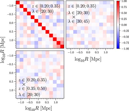
Jackknife-estimated correlation matrix of |$\widetilde{\Delta \Sigma }$| of a single richness-redshift selection with |$\lambda \in [20;\, 30)$| and |$z \in [0.2;\, 0.35)$|(upper left panel). The off-diagonal blocks display the correlation matrix between the reference profile and the neighbouring richness bin |$\lambda \in [30;\, 45)$|(upper right panel), and the neighbouring redshift bin |$z \in [0.35;\, 0.5)$|(lower left panel).
3.2.1 Shape noise
The large intrinsic variations of the shapes of galaxies (shape noise) in the source catalogue constitute a dominant source of uncertainty in lensing measurements. We estimate the covariance originating from both the random intrinsic alignments and also the stochastic positions of source galaxies. In order to do so, we make use of the measurement setup outlined in Section 3.1.3, but each source is randomly rotated to create a new source catalogue. We generated 1000 such independent rotated source catalogues, and performed the lensing measurement with each. The resulting data vectors are consistent with zero, as the random rotation washes away the imprint of the weak lensing signal. However, their scatter is indicative of the covariance due to shape noise.
We estimate the shape noise covariance matrix for each of the 1000 realizations using the spatial jackknife scheme outlined above in Section 3.2. The final shape noise covariance matrix estimate is obtained by averaging all 1000 of these jackknife covariance matrices. We expect this method to be less noisy compared to estimating the covariance matrix from the 1000 independent measurements of the rotated ΔΣ vector only.
3.2.2 Uncorrelated LSS
Naively, one would expect that the variance of a cluster stack due to uncorrelated large-scale structure to scale simply as 1/Nclusters. In practice, however, the positions of galaxy clusters are correlated, and the area around them overlaps on large scales. Consequently, we expect the variance due to uncorrelated structure to decrease somewhat more slowly than 1/Nclusters.
We estimate this source of noise by measuring random realizations of the signal due to shear fields induced by lognormal density fields with the appropriate power spectra and skewness. We calculate the latter with the perturbation theory model of Friedrich et al. (2018) for the Buzzard cosmology (DeRose et al., in preparation; Wechsler, DeRose & Busha, in preparation), using the lognormal parameter κ0 at a 10’ aperture radius. As our cluster sample spans a range in redshift, a different shear field is calculated for each of the three redshift bins. This is done such that the shear fields are calculated at the lens-weighted mean source galaxy redshifts found during the initial measurement in Section 3.1.3. We then pass these shear fields through the measurement pipeline using a spatial mask reflecting the actual source number density variations across the footprint, and estimate the covariance matrix for each realization using 100 spatial jackknife regions for each bin in richness and redshift.
This above procedure was repeated 300 times, and the final covariance matrix due to uncorrelated LSS is taken to be the mean of the 300 jackknife covariance estimates.
3.2.3 Correlated LSS and halo ellipticity
3.2.4 M–c scatter, M-λ scatter and miscentring
Halos at a given mass have some intrinsic scatter in their M–λ relation. A rough estimate of the intrinsic scatter in the mass–richness (M–λ) relation is ∼ 25 per cent (Rozo & Rykoff 2014; Farahi et al., in preparation), and it causes an increase in the variance of stacked measurements of ΔΣ. This scatter causes an even larger increase in the variance, since it propagates into quantities that depend directly on the mass, including the M–c relation. In addition, concentration (e.g. Bhattacharya et al. 2013; Diemer & Kravtsov 2015) and miscentring possess some intrinsic scatter from halo to halo themselves.
Scatter in the M–λ relation causes variance on all scales, since the bias b(M) directly depends on the mass. By comparison, scatter in the M–c relation primarily affects small scales where the 1-halo term dominates. Similarly, some cluster centres are misidentified in our stacks, which creates additional covariance at small scales where the signal is substantially suppressed.
We modelled the combined contribution to the SAC from scatter in M–λ, scatter in concentration at fixed mass, and miscentring of individual clusters in our stacks by doing the following:
For each cluster in our stack, assign a mass by inverting a fiducial M–λ relation (Melchior et al. 2017) and assuming 25 per cent scatter. This is not identical to 25 per cent scatter in the M–λ relation; however. this choice negligibly affects this component of the covariance matrix.
For each cluster, assign a concentration (including scatter) based on Diemer & Kravtsov (2015).
For each cluster, make a draw from our centring prior described in Section 5.2. In other words, some fraction fmis of clusters in the stack are miscentred, and the distribution of the amount of miscentring is given by p(Rmis).
Calculate ΔΣ for each cluster and average these signals to generate a signal for the entire stack.
Repeat this process many times, and use these independent realizations to estimate the corresponding covariance matrix between the various radial bins.
Using Simet et al. (2017) as our fiducial M–λ relation or using the Bhattacharya et al. (2013) mass–concentration relation had no impact on the final SAC matrix. We have also verified that using half as many realizations as our fiducial choice (1000) did not appreciably change the resulting covariance matrix. The same is true for changes in the richness scatter or miscentering model parameters within reasonable ranges.
3.2.5 Semi-analytic covariance matrix
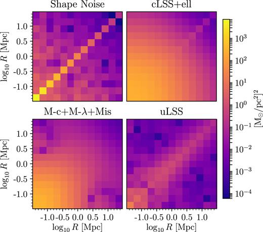
The four individual components to our semi-analytic ovariance (SAC) matrix. Clockwise from top left: Shape noise component from randomly rotating sources, correlated LSS and ellipticity component from integrating over configurations of the host cluster and its correlated halos, uncorrelated LSS from integrating over large-scale structure, and finally scatter in the M−λ relation, M−c relation, and miscentering distribution. Dark colours correspond to low covariance and the colours are log-scaled to show trends. Light colours are normalized to the total covariance in the SAC. See Section 3.2 for details.
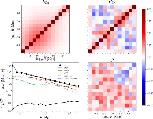
Comparison between the semi-analytic covariance matrix and the jackknife-estimated covariance matrix. Top left: Correlation matrix of the SAC matrix. Top-right: Correlation matrix of the jackknife estimate. Bottom left: Comparison of the errors in the SAC and jackknife estimate along with the contributions to the SAC error from each individual component. The line showing the SAC errors lies almost on top of the shape noise contribution, confirming that it is the dominant source of covariance. Bottom right: Residual matrix Q (see equation 22) that represents the difference between the SAC and jackknife covariance matrices. See Section 3.2 for details.
Using the SACs in our analysis provides two major improvements: minimal bias from inverting the covariance matrix, and less overall noise in the off-diagonal elements which improves the mass measurement. In Melchior et al. (2017), we demonstrated that noise in the jackknife covariance matrix led to an increase of ≈30 per cent in the uncertainty of the mass of the stack. Using the SACs reduces the contribution of the covariance to the error budget by 10 per cent compared to the jackknife-estimated covariance.
4 SYSTEMATICS
4.1 Shear systematics
The metacalibration shear catalogue and the associated calibration of the source redshift distributions (Hoyle et al. 2018) passed a large number of tests performed by Zuntz et al. (2018) and Prat et al. (2018). Here, we briefly enumerate the constraints on the most relevant systematics, and refer the reader to the corresponding papers for a more detailed analysis.
In weak lensing surveys, the three main sources of bias are commonly found to be model bias, noise bias, and selection bias (or representativeness bias). In order to account and correct for these sources of error, the metacalibration algorithm performs a self-calibration on the actual data by shearing the galaxy images during the measurement, and using the thus-calculated responses to correct the shear estimates. To quantify the effectiveness of this self-calibration, Zuntz et al. (2018) ran the metacalibration pipeline on a set of simulated galaxy images using GalSim (Rowe et al. 2015). The images were produced from high-resolution galaxy images from the COSMOS sample, and processed to resemble the actual DES Y1 observations both in noise and PSF properties. Based on this test scenario, Zuntz et al. (2018) found no significant multiplicative bias m or additive bias c present in the data set.
Zuntz et al. (2018) further investigated the multiplicative biases due to blending of galaxy images, due to the potential leakage of stellar objects into the galaxy sample, and due to potential errors in the modelling of the PSF. They found blending as the only component with a net bias, with the other sources being consistent with zero, although contributing to the uncertainty on the value of m. The final multiplicative bias estimates were found to be m = [1.2 ± 1.3] · 10−2 with a 1σ Gaussian error. They found no evidence of a significant additive bias term.
Prat et al. (2018) tested for the presence of residual shear calibration biases in the DES Y1 galaxy-galaxy lensing analysis by splitting the source sample by various galaxy properties and parameters of the observational data. They showed that within the statistical uncertainty of the respective galaxy–galaxy lensing signals, and including the differences in redshift distributions induced by the splitting, no differential multiplicative biases between any of the splits were significantly detected.
In addition to the above calibrations during the construction of the shear catalogue, we perform additional sanity checks relevant to stacked weak lensing measurements in the subsections below.
4.1.1 Second order shear bias
The choice of α = 0.6 in our test is motivated by the image simulations used in Sheldon & Huff (2017). Other simulations find a range of values of similar magnitude. Since the effect is smaller than the overall shear uncertainty, yet its calibration is uncertain, we choose not to implement a correction in our final model.
4.1.2 B-modes
Gravitational lensing due to localized mass distributions can only produce a net E-mode signal in the shear field, which corresponds to the tangential shear γt. This allows for a simple null test for the presence of systematics: any non-zero cross-shear (i.e. a non-zero B-mode) must be due to systematics. We compute the cross-shear by projecting the shears to the direction 45° from the tangential direction. We estimate the stacked B-mode signal for all richness and redshift bins, and calculate the corresponding χ2 values using the jackknife estimate of the covariance matrix. We find χ2/11 < 18/11 for all richness bins with λ > 20, indicating that our measurement is consistent with no systematics at a p > 0.1 level.
4.1.3 Random point test
In spite of not being detected by Zuntz et al. (2018) and Section 4.1.2, additive shear systematics may be present in the data, which could manifest as net signals visible on all radial scales. In order to test for such potential systematics, we measure the lensing signal around a set of random points chosen by the redMaPPer algorithm (Rykoff et al. 2016). These points are selected via weighted random draws to mirror the distribution of DES Y1 redMaPPer clusters both in angular distribution, as well as in redshift and richness.
As additive systematics would affect the lensing profiles of galaxy clusters and random points the same way, the systematic effect can be calibrated out by subtracting the profile of random points from the profile of clusters. While we find no significant net signal around random points, we nevertheless apply this calibration, and subtract the signal of 105 random points from the |$\widetilde{\Delta \Sigma }$| of each bin in richness and redshift. Thanks to the large number of random points used, this subtraction does not introduce significant noise to the measurement.
A motivation for subtracting the signal around random points from the measurement, regardless of the presence of systematics, is presented by Singh et al. (2016). They found that the random subtracted signal relates to the matter over-density field around the lenses, while the un-subtracted lensing signal traces the matter density field, which carries additional variance on large scales. Indeed, the precursor study of the present paper (Melchior et al. 2017) found a similar trend. We note that when constructing our SAC matrix we always apply the random point subtraction described above to ensure that our covariance matrix properly accounts for the reduced covariance that this estimator enables.
4.2 Correction for cluster members in the shear catalog
Due to uncertainty in photometric redshift estimates, foreground galaxies can be included in the source catalogue used in our lensing measurements. So long as the ensemble redshift distribution dn/d|$z$| of the sources is properly estimated, this is accounted for in our analysis. In the projected vicinity of galaxy clusters, there is however a systematic effect biasing the naive redshift estimates of galaxies: the presence of a large cluster member population and the associated large-scale matter overdensity localized at the cluster redshift. For rich clusters, these member galaxies could make up a significant fraction of all detected galaxies in a particular line of sight. Consequently, due to intrinsic imperfections in the selection, some of these galaxies leak into the source catalog used in the weak lensing measurement. Cluster member galaxies are randomly aligned (Sifón et al. 2015), meaning their contamination results in a measured lensing signal which is biased low due to the dilution of actual source galaxies within the catalogue.
It is therefore important for weak lensing studies to characterize and correct this dilution when interpreting the measurements.4 There have been several approaches in the literature to correct for the net effect of cluster member contamination. For instance, Sheldon et al. (2004) estimated the correction factor from the transverse correlation of source galaxies around galaxy clusters, while Gruen et al. (2014) and Melchior et al. (2017) estimated the contamination rate based on the colour or photometric redshift p(|$z$|) information of galaxies in different radial separations from the cluster. One can also make simple colour cuts (Medezinski et al. 2010, 2018a; Schrabback et al. 2018) or photo-|$z$| cuts (Applegate et al. 2014) on the source population to mitigate the contamination, or estimate its effect based on the increased galaxy number density around the lenses (Hoekstra et al. 2015; Simet et al. 2015; Dietrich et al. 2017).
4.3 Photometric redshift systematics
The redshift distribution of our selected source galaxies was estimated using BPZ (Benítez 2000) in the implementation of Hoyle et al. (2018). In BPZ or similar photometric redshift estimation procedures, one assumes a variety of galaxy spectral energy distribution (SED) templates and priors for the relative abundance of galaxies as a function of luminosity and redshift. Any deviation from these assumptions in the DES source galaxy sample can cause biases in photometric redshift estimates which must be calibrated.
For the cosmology analyses of the lensing two-point functions (Dark Energy Survey Collaboration 2016; Troxel et al. 2018), this calibration was performed in two independent ways, and with consistent results: by the redshift distributions of samples of galaxies with high-quality 30-band photo-|$z$|s from COSMOS, matched to DES lensing source galaxies (Hoyle et al. 2018), and by the clustering of lensing source galaxies with redMaGiC (Rozo et al. 2016) galaxies as a function of the redshift of the latter (Davis et al. 2018; Gatti et al. 2018).
For this work, we adapt the COSMOS calibration of Hoyle et al. (2018) to estimate the bias of our ΔΣ measurements, and the uncertainty in that bias. To this end, we select and weight galaxies from COSMOS in the same manner as for our measurements of the cluster ΔΣ profiles.
Following Hoyle et al. (2018, their section 4.1), we randomly sample 200 000 galaxies in our data and match them to COSMOS galaxies according to their flux in each band and their intrinsic size. From this COSMOS resampling, we select and weight galaxies as per Sections 3.1.2 and 3.1.3. From the COSMOS 30-band, we calculate the weighted mean true |$\Sigma _{\rm crit,TRUE}^{^{\prime }-1}$|. From noisy MOF grizbpz redshift distribution samples, we get a mean |$\Sigma _{\rm crit, MEAS}^{^{\prime }-1}$| that relates the weighted mean tangential shear to the ΔΣ profile. As in the denominator of equation (12), we use a weight |$\omega \times \mathsf {R}$| for the means. Because the source selection, ω weight, and |$\Sigma _{\rm crit}^{^{\prime }}$| depends on lens redshift, we repeat this exercise for the range of cluster redshifts sampled by our catalogue, |$z$|l = 0.2…0.65. A bias in |$\Sigma _{\rm crit}^{^{\prime }-1}$| translates directly into a multiplicative bias in ΔΣ.
We estimate four sources of uncertainty in the calibration of photometric redshift distributions (see Hoyle et al. 2018, their sections 4.2–4.5): 1) an uncertainty due to cosmic variance from the relative scatter of average |$\Sigma _{\rm crit,TRUE}^{^{\prime }-1}$| in the resampling of the 368 simulated COSMOS footprints, to which we add the (subdominant) statistical uncertainty due to the limited sample size from bootstrap resamplings in quadrature; 2) an uncertainty due to photometric zeropoint offsets from realizations of photometric zeropoint calibration offsets; 3) an uncertainty due to the morphology matching, which we estimate as half the difference between the estimated |$\Sigma _{\rm crit,TRUE}^{^{\prime }-1}$| of the sample with size + flux matching and that obtained without the size matching; and 4) a systematic uncertainty of the matching algorithm by a comparison between the fiducial |$\Sigma _{\rm crit,TRUE}^{^{\prime }-1}$| value and that of the aforementioned 368 resampled simulated COSMOS fields. Effects 1, 3, and 4 contribute to the systematic uncertainties with similar size, while effect 2 is smaller but not quite negligible.
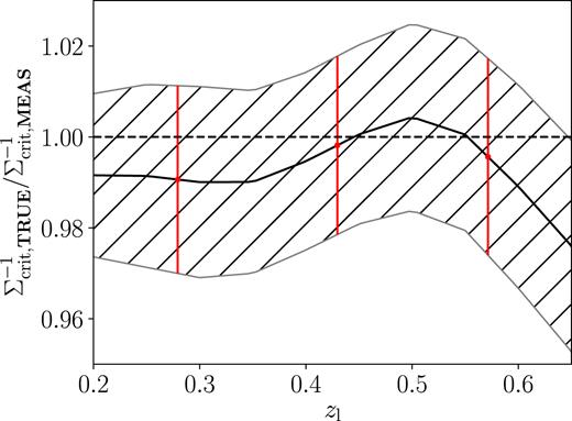
The photo-z correction factor to |$\Sigma _{\rm crit}^{-1}$| as described in Section 4.3. The grey hatched region indicates the 1σ range of the correction factor. Red points with error bars show the correction factors applied to each redshift bin.
An additional concern is the effect of intra-cluster light leaking into source photometry used for redshift estimation. We test for this in Gruen et al. (in preparation) with the intra-cluster light measurements of Zhang et al. (in preparation), finding negligible effects in the regimes relevant for this study.
5 THE STACKED LENSING SIGNAL
5.1 Surface density model
| Parameter | Description | Prior |
|---|---|---|
| log10M200m | Halo mass | [11.0, 18.0] |
| c200m | Concentration | [0, 20] |
| τ | Dimensionless miscentering offset | 0.17 ± 0.04 |
| fmis | Miscentered fraction | 0.25 ± 0.08 |
| Am | Shape & photo-|$z$| bias | equation (45) |
| |$B_0^{\rm cl}$| | Boost magnitude | [0, ∞] |
| |$R_s^{\rm cl}$| | Boost factor scale radius | [0, ∞] |
5.2 Miscentring correction
5.3 Multiplicative corrections
5.3.1 Boost factor model
5.3.2 Reduced Shear
5.3.3 Shear + photo-|$z$| bias
The factor |$\mathcal {A}_m = 1 + m + \delta$| combines the effects of shear (m, Section 4.1) and photo-|$z$| (δ, Section 4.3) systematic uncertainties. Zuntz et al. (2018) found a shear calibration of m = 0.012 ± 0.013. The photo-|$z$| bias comes from Hoyle et al. (2018) and varies between cluster stacks.
For the following data releases of DES, we anticipate that improvements in the treatment of blended objects can further reduce the multiplicative shear bias. This implies that uncertainties in the calibration of photometric redshift estimates will likely be our dominant measurement related systematic. Significant improvements on this will require either extended calibration data sets or a hierarchical treatment that uses survey data to inform redshift estimation consistently.
5.4 Stacked mass corrections
We expect the masses we measure in Section 5.5 to be biased with respect to the true mean mass of the stacks. This bias arises from two sources: our model presented above is not a true description of cluster lensing profiles, and effects due to triaxiality and projection. We account for both sources of bias by calculating a correction |$\cal {C}$| applied to the expected mass of the stack |$\mathcal {M}_{\rm true} = \mathcal {C}\langle M\rangle$|, as detailed in the section below. This is applied after the lens modelling is complete, but before modelling the mass–observable relation from our stacked masses in Section 6.
5.4.1 Modelling systematics
The model presented above for ΔΣ is not perfect; our analytic model for the halo–mass correlation function in equation (31) does not match density profiles in simulations (Melchior et al. 2017; Murata et al. 2018), in particular, in the transition between the 1-halo and 2-halo regimes. In lieu of a fully calibrated model, we correct for any bias imparted by our choice of model by using our likelihood analysis to estimate halo masses of synthetic data generated from N-body simulations. The haloes are drawn from an N-body simulation of a flat ΛCDM cosmology run with Gadget (Springel 2005). The simulation uses 14003 particles in a box with 1050 h−1Mpc on a side with periodic boundary conditions and for softening of 20 h−1kpc. The simulation was run with the cosmology Ωm = 0.318, h = 0.6704, Ωb = 0.049, τ = 0.08, ns = 0.962, and σ8 = 0.835. Halos of mass 1013 h−1M⊙ are resolved with 100 particles. We discard all information below five softening lengths, and verified that the choice of extrapolation scheme for describing the correlation function below this scale does not impact our results. Halos were defined using a spherical overdensity mass definition of 200 times the background density and were identified with the rockstar halo finder (Behroozi et al. 2013).
The simulation is used to construct the synthetic ΔΣ profiles of galaxy clusters at four different snapshots: |$z$| ∈ [0, 0.25, 0.5, 1]. There were ∼420 000 haloes at |$z$| = 1 and ∼830 000 haloes at |$z$| = 0. We used snapshots instead of lightcones for two main reasons: we wanted to maximize the number of haloes we had available to perform the calibration, and we found that the synthetic profiles to only weakly depend on redshift. Instead of splitting haloes into mass subsets as in Melchior et al. (2017), we assigned a richness to each halo by inverting the mass–richness relation of Melchior et al. (2017) and adding 25 per cent scatter. We then grouped our haloes into richness subsets identical to how we grouped our clusters. For each of these halo subsets, we measured the halo–matter correlation function with the Landy & Szalay (1993) estimator as implemented in Corrfunc6 (Sinha & Garrison 2017). We numerically integrate the halo–matter correlation function to obtain the ΔΣ profile as described in Section 5.1.
This ΔΣ profile contains none of the systematics that exist in the real data. To incorporate them, we modified this profile with the multiplicative corrections described in Section 5.3 and miscentering corrections in Section 5.2. We took the central values of our priors in Table 1 as well as values for B0 and Rs from modelling the boost factors independently and modified the simulated ΔΣ profile according to equation (47). The observed mass Mobs for this simulated profile was obtained by using the same pipeline that we apply on the real data. When evaluating the likelihood in equation (50), we used the semi-analytic covariance matrix corresponding to the nearest cluster subset in redshift.
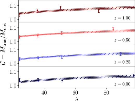
The mass calibration |$\mathcal {C} = M_{\rm true}/M_{\rm obs}$| from adopting our model of the correlation function in equation (31) as a function of λ and redshift. The solid line and hatched region are the best-fit model and 1σ uncertainty of the calibration. Error bars on the measured calibrations are the fitted intrinsic scatter |$\sigma _{\mathcal {C}}$|.
We incorporated the dependence of the calibration on the intrinsic scatter in the M–λ relation as follows. We took the calibration described above at 25 per cent scatter to be our fiducial model as estimated in Rozo & Rykoff (2014). In addition to the covariance between C0, α, and β, we add additional uncorrelated uncertainty to each of these terms equal to half of the difference between the mean values obtained for these parameters assuming 15 per cent and 45 per cent scatter. This increased the variance of all three parameters C0, α, and β slightly. As discussed further in 8, the calibration contributed 0.73 per cent to the overall systematic uncertainty on the normalization of the M–λ relation.
One effect which we have not explicitly accounted for is the impact of baryonic physics on the recovered weak lensing masses. Baryonic cooling and feedback leads to mass redistribution in the central regions of galaxy clusters, with the impact of baryonic physics decreasing with increasing radius. Given that our fits allowed the concentration parameter of each cluster stack to float with no informative priors, we naively expect the impact of baryonic physics can be absorbed into the concentration of each cluster stack (Schaller et al. 2015). This naive expectation is confirmed in the work of Henson et al. (2017), who found that while baryonic physics impact the recovered weak lensing masses, the relative bias between the recovered weak lensing mass and the true mass is roughly constant, independent of baryonic physics. Given that we measure masses at large radii (R200m), and in light of the above results, we believe the impact of baryonic physics is likely to be less than |${\sim } 3{{\ \rm per\ cent}}$| or so. Future work in which we explicitly test our fitting routines using hydrodynamic simulations is clearly desirable.
5.4.2 Triaxiality and projection effects
Photometric cluster selection preferentially selects haloes that are oriented with their major axis along the line of sight. Similarly, cluster selection is affected by other objects along the line of sight, which increases both the observed cluster richness and the recovered lensing mass. These two effects have been studied closely elsewhere (White et al. 2011; Angulo et al. 2012; Noh & Cohn 2012; Dietrich et al. 2014), and have competing effects on the recovered cluster masses. Dietrich et al. (2014) determined that triaxiality leads to an overestimation of the weak lensing mass and requires a correction factor of 0.96 ± 0.02, while Simet et al. (2017) argued projection effects require that the recovered masses be multiplied by a factor of 1.02 ± 0.02. Together, triaxiality and projection effects modify the recovered weak lensing masses by a multiplicative factor of 0.98 ± 0.03. Our treatment is identical to that of Melchior et al. (2017), where additional details are provided. Although these two effects mildly depend on richness and redshift, we assume them to be constant in this analysis. We show the cumulative effect in Table 6. For reference, we have estimated the number of galaxy clusters that have another cluster within a 500 kpc radius along the line of sight. The number of such cases with λ ≥ 20 is about 30, or 0.4 per cent of our sample, and thus negligible.
These effects as well as the correction for model bias are applied to the masses after fitting the lensing and boost factor data as described in Section 5.5, but before modelling the M–λ relation in Section 6.
5.5 The complete likelihood
5.6 Stacked cluster masses
A complete list of the model parameters describing each cluster stack as well as their corresponding priors are summarized in Table 1. The likelihood is sampled using the package emcee7 (Foreman-Mackey et al. 2013), which enables a parallelized exploration of the parameter space. We use 32 walkers with 10000 steps each, discarding the first 1000 steps of each walker as burn-in. We checked the convergence with independent runs of 5000 steps per walker that yielded identical results. After 14 steps the chains of single walkers become uncorrelated (with a correlation coefficient |r| < 0.1). This is much shorter than the total length of the chain. As a result, the number of independent draws between all walkers is ≈20500.
In order to characterize the contribution of both statistical and systematic uncertainties to our final results we perform our analysis three different times with three different sets of assumptions. These three analyses we run are:
Full: All parameters (concentration, Shear + photo-|$z$|, boost factors, miscentering) are allowed to vary within their priors. This is our fiducial analysis.
FixedAm: |$\mathcal {A}_m$| is set to the center of its prior distribution but all other parameters are allowed to vary. This determines the contribution from the shape and photo-|$z$| uncertainties.
OnlyMc: Only mass and concentration are free. All other parameter priors are set to δ-functions at their central values. This represents our statistical uncertainty on the mass.
Table 2 contains the results of the Full analysis. Full posteriors from the cluster subset |$z$| ∈ [0.2, 0.35) and λ ∈ [20, 30) are shown in Fig. 10. The corresponding data and best-fit model are shown in Fig. 11, where we also demonstrate the combined effects of miscentering, boost factors, reduced shear, and multiplicative bias. The best-fit model for each richness and redshift bin is over-plotted on top of the weak lensing data in Fig. 4.
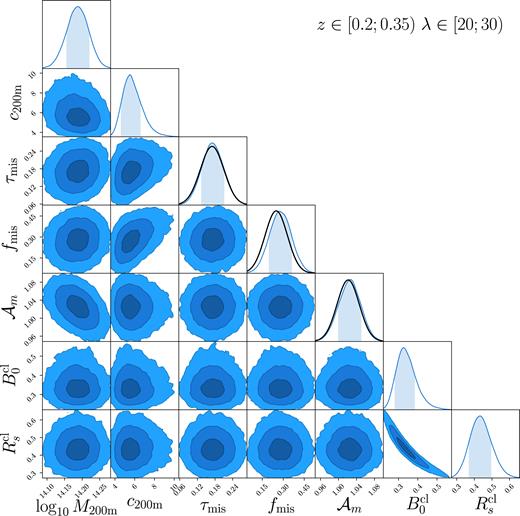
Posteriors for the parameters describing the lensing profile ΔΣ and the boost factor profile |$\mathcal {B}$| for the bin |$z$| ∈ [0.2, 0.35), λ ∈ [20, 30). Contours show the 1σ, 2σ, and 3σ confidence areas. Black lines show the prior distributions. The mass presented here is uncalibrated, meaning it has not been corrected for modelling systematics, projection effects, or cluster triaxiality (see Section 5.4).
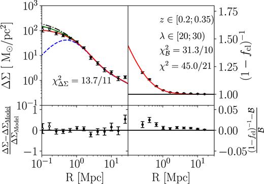
Fit with all components of the ΔΣ and |$\mathcal {B}$| models for the cluster subset |$z$| ∈ [0.2, 0.35) and λ ∈ [20, 30). The top two panels show the best-fit models in red compared to the data. Unfilled points are not included in the fit. Top left: the black dot–dashed line is ΔΣcen while the blue–dashed line is ΔΣmis. The weighted mean of these two yields the green solid line, and then applying the boost factor model, reduced shear, and multiplicative bias yields the final model in red. Top right: the red line is our NFW model for the boost factors. Bottom: the fractional difference between our data and models. The total χ2 is 45 with 21 degrees of freedom, which is acceptable despite the imperfect fit of our simple model to the boost factors. The boost factors are measured from the data with small uncertainty, which is why the small mismatch with respect to the best-fit model causes a relatively large χ2 but negligible effect on the recovered mass.
Calibrated masses for each richness–redshift stack. All masses are in units of log10M⊙ using the M200m definition. Listed uncertainties are split into the symmetric 68 per cent confidence intervals of the systematic and statistical components, in that order. Adding the two in quadrature gives the total uncertainty on the mass.
| λ | |$z$| ∈ [0.2, 0.35) | |$z$| ∈ [0.35, 0.5) | |$z$| ∈ [0.5, 0.65) |
|---|---|---|---|
| [20, 30) | 14.191 ± 0.013 ± 0.032 | 14.162 ± 0.013 ± 0.033 | 14.083 ± 0.015 ± 0.048 |
| [30, 45) | 14.477 ± 0.014 ± 0.031 | 14.446 ± 0.014 ± 0.031 | 14.456 ± 0.015 ± 0.041 |
| [45, 60) | 14.608 ± 0.011 ± 0.044 | 14.643 ± 0.011 ± 0.044 | 14.648 ± 0.016 ± 0.056 |
| [60, ∞) | 14.913 ± 0.014 ± 0.038 | 14.899 ± 0.015 ± 0.038 | 14.879 ± 0.023 ± 0.061 |
From the Full analysis we can see the contribution of the various systematics to our final results. The boost factors amount to a correction of ≈2 per cent to ΔΣ at R = 1 Mpc. The posteriors on the miscentering parameters are equal to the priors, demonstrating that these parameters are only weakly constrained by the weak lensing data. In our earlier analysis (Melchior et al. 2017), we found a weak correlation between fmis and M, which did not appear in this work. This was due to our use of the Diemer & Kravtsov (2014) M–c relation. We determined this by running one additional configuration in which the concentration was fixed by the Diemer & Kravtsov (2014) M–c relation, thus increasing the correlation between fmis and M. At present, the contribution of miscentering to the mass is sub-dominant to other sources of systematic uncertainties in our final error budget (cf. Table 6). The multiplicative bias |$\mathcal {A}_m$| follows the prior and is degenerate with mass.
The OnlyMc likelihood evaluation allows us to quantify the statistical and systematic uncertainties of the fiducial analysis. The difference in quadrature between the uncertainties in the Full and OnlyMc configurations represents the total systematic contribution to the error budget, while the OnlyMc alone provides the statistical contribution. The central values for each cluster subset along with statistical and systematic contributions to the uncertainties are presented in Table 2.
6 THE MASS–RICHNESS–REDSHIFT RELATION
The quantity we aim to constrain in this paper is the mean mass |$\mathcal {M}(\lambda ,z)$| of clusters of galaxies at a given observed richness λ and redshift |$z$|, similar to what was done in Melchior et al. (2015). Note that this is different from constraining the mean (and possibly distribution) of richness at given mass, or the full distribution of mass at given richness, as done in, e.g. Simet et al. (2017) amd Murata et al. (2018). In particular, we neither constrain nor require a model of the intrinsic scatter in richness, hence making this analysis largely independent from the choices in subsequent cluster cosmology studies based upon it.
We note that an assumed value of the intrinsic scatter is used in two places: the semi-analytic covariance matrices described in Section 3.2.5 and the calibration described in Section 5.4.1. For the covariance, this assumption had a negligible effect compared to the shape noise. While the overall calibration did depend on the amount of scatter, we took a conservative approach by treating the difference in calibration between assuming 15 per cent and 45 per cent scatter as a systematic uncertainty. In this way, our final results are not sensitive to the amount of assumed intrinsic scatter.
6.1 Modelling the mass–richness relation
The logarithm of the mean mass correction factor log10a from equation (54). This represents a correction to the stacked cluster masses due to the fact that different clusters contribute to the measured mass in a different way than they contribute to ΔΣ.
| λ | |$z$| ∈ [0.2, 0.35) | |$z$| ∈ [0.35, 0.5) | |$z$| ∈ [0.5, 0.65) |
|---|---|---|---|
| [20, 30) | −1.372 × 10⁻³ | −8.744 × 10⁻⁴ | −4.501 × 10⁻⁴ |
| [30, 45) | −2.979 × 10⁻³ | −3.278 × 10⁻³ | −6.660 × 10⁻⁴ |
| [45, 60) | −8.258 × 10⁻⁴ | −7.856 × 10⁻⁵ | −1.903 × 10⁻³ |
| [60, ∞) | 3.043 × 10⁻³ | −4.061 × 10⁻³ | 6.264 × 10⁻³ |
6.2 Mass covariance
The purpose of our different chain configurations (Full, FixedAm, and OnlyMc) is to allow us to estimate the contribution of each systematic to the final uncertainty on the mass calibration parameters M0, Fλ, and G|$z$|. In our analysis, there are seven sources of systematic uncertainty: multiplicative shear bias, multiplicative photo-|$z$| bias, miscentering, boost factors, modelling systematics, triaxiality and projection.
6.3 Likelihood for the mass–observable relation
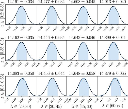
The calibrated posteriors of the masses for each cluster stack. Uncertainties appear above each panel, and are highlighted by the blue-regions. Gaussian approximations to these posteriors appear as black dashed lines.
We sample the posterior of the MOR parameters using emcee with 48 walkers taking 10000 steps each, discarding the first 1000 steps of each walker as burn-in. Table 4 summarizes the posteriors of our model parameters, while Fig. 13 shows the corresponding confidence con tours. All parameters in the M–λ–|$z$| relation have flat priors.
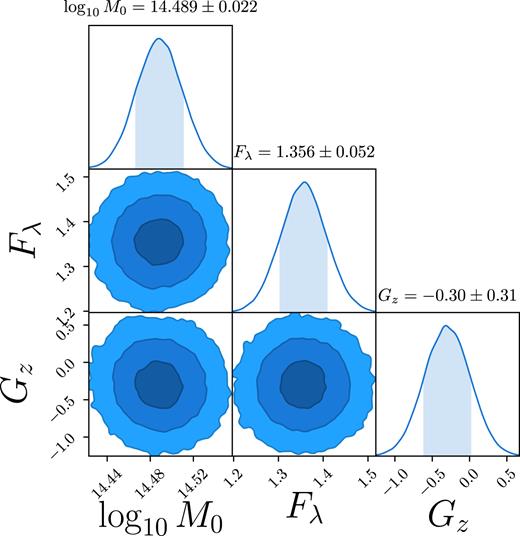
Parameters of the M–λ–|$z$| relation. Contours show the 1σ, 2σ and 3σ confidence areas from the Full run.
Parameters of the M–λ–|$z$| relation from equation (64) with their posteriors. The mass is defined as M200m in units of M⊙. The pivot richness and pivot redshift correspond to the median values of the cluster sample. Uncertainties are the 68 per cent confidence intervals and are split into statistical (first) and systematic (second).
| Parameter | Description | Posterior |
|---|---|---|
| log10M0 | Mass pivot | 14.489 ± 0.011 ± 0.019 |
| Fλ | Richness scaling | 1.356 ± 0.051 ± 0.008 |
| G|$z$| | Redshift scaling | −0.30 ± 0.30 ± 0.06 |
| Parameter | Description | Posterior |
|---|---|---|
| log10M0 | Mass pivot | 14.489 ± 0.011 ± 0.019 |
| Fλ | Richness scaling | 1.356 ± 0.051 ± 0.008 |
| G|$z$| | Redshift scaling | −0.30 ± 0.30 ± 0.06 |
We explicitly enforce correlated uncertainties of shear, photo-|$z$|, modelling systematics, and triaxiality and projection effects. Miscentering and boost factors are considered independent across cluster subsets. These independent uncorrelated systematics will tend to average out across bins.
In order to distinguish between the systematic and statistical contribution to the error budget on the M–λ–|$z$| relation parameters, we repeat the analysis using the statistical errors from the OnlyMc run. That is, we calculate equation (64) using only the uncertainties measured from the OnlyMc run, or the |$\mathsf {C}^{\rm stat}_M$| covariance matrix. The central values of the measured masses from the OnlyMc run are nearly identical to the Full run, as are the parameters in the M–λ–|$z$| relation. The difference in quadrature between the two uncertainties represents the systematic contribution while the excess uncertainty from the OnlyMc run is the statistical contribution. These uncertainties are reported in Table 4.
Our results imply that galaxy clusters of richness λ = 40 at redshift |$z$| = 0.35 have a mean mass of |$\log _{10} {\cal M}= 14.489\ \pm 0.011\ {\rm (stat)}\ \pm 0.019\ {\rm (sys)}$|. The richness scaling is slightly steeper than linear at Fλ = 1.356 ± 0.051 (stat) ± 0.008 (sys), while the mass shows a weak redshift dependence of G|$z$| = −0.30 ± 0.30 (stat) ± 0.06 (sys) consistent with no evolution. This amounts to a 5.0 per cent calibration (2.4 per cent statistical, 4.3 per cent systematic), of the normalization of the M–λ–|$z$| relation.
In Melchior et al. (2017), we found that the dominant systematic uncertainty stemmed from shear and photo-|$z$| systematics, as was the case in Simet et al. (2017). By repeating our analysis with the FixedAm run, which includes all systematics except|$\mathcal {A}_m$|, we are able to quantify the contribution from these sources. We found that the posterior distributions from the M–λ–|$z$| relation are significantly reduced, and that shear and photo-|$z$| systematics alone account for 48 per cent of the systematic uncertainty. This means that the remaining 52 per cent of the systematic uncertainty is due to modelling systematics, projection effects, and cluster triaxiality.
6.3.1 Alternative model using ξlin
Hayashi & White (2008) used a similar model to ours, but with the linear matter correlation function for their 2-halo term. This causes a very different behaviour near the 1-halo to 2-halo transition region, which can affect the fitting procedure, as discussed in Melchior et al. (2017). We repeated our entire analysis, including recomputing the calibration, using ξlin in place of ξnl. The masses of the stacks changed by less than 1 per cent, as did the normalization of the M–λ relation log10M0. This means that our approach of calibrating the masses is largely robust to our choice of model.
6.3.2 Additional tests
We performed additional tests to verify our results. To ensure against possible small-scale systematic effects, we repeated our analysis with a more conservative radial cut of 500 kpc rather than 200 kpc. The resulting M–λ–|$z$| relation changed only in the mass scale, with M0 changing by 0.2σ.
We also tested against possible differences in modelling systematics between large and small scales. By dividing each ΔΣ profile at 2 Mpc into large and small scale samples we could fit these regimes independently. While the constraining power was greatly diminished, the recovered masses were consistent with each other and the fiducial value within errors. No trend was observed in the differences between the recovered masses in any of these tests compared to the fiducial masses in Table 2.
Lastly, we tested an extension of equation (52) where Fλ(|$z$|) = Fλ, 0 + zFλ, 1 and found Fλ, 1 consistent with 0 at the 1.2σ level. Therefore, if any redshift evolution exists in the richness scaling, we are unable to resolve the behaviour at present.
7 COMPARISON TO RESULTS IN THE LITERATURE
We compare our calibration of the M–λ relation to previous results from the literature. The specific richness–mass relations we consider are summarized in Table 5, and we describe below the origin of each of these.
Melchior et al. (2017) was the precursor to this analysis. In that work, we calibrated the mass–richness relation of redMaPPer clusters in the DES Science Verification data. A detailed description of the changes between that analysis and this one appears in the next section.
Baxter et al. (2018) used the lensing of the Cosmic Microwave Background as measured by the South Pole Telescope to measure the mass–richness relation of DES Y1 redMaPPer clusters. Their analysis focused on 7066 clusters with richness 20 ≤ λ ≤ 40. The upper limit was set to avoid potential biases in the recovered masses from contamination by thermal Sunyuaev-Zel’dovich emission by the clusters.
Simet et al. (2017) measured the mass–richness relation of redMaPPer clusters found in the Sloan Digital Sky Survey (SDSS). While their analysis is similar in spirit to ours, there are numerous methodological differences, including modelling choices (Simet et al. only fit the 1-halo term in the lensing profile), different radial scales used in the fit, a different shape catalog, and different photometric redshift catalogs.
Murata et al. (2018) measured the richness–mass relation of SDSS redMaPPer clusters assuming a Planck cosmology. We compute the mean mass at λ = 40 as well as the local slope at this point in the scaling relation. As demonstrated in Murata et al. (2018), their work and Simet et al. (2017) are consistent with each other, despite the fact that they used different models for ΔΣ, different radial scales and slightly different richness bins. Of special note is the fact that while Simet et al. (2017) modelled only the 1-halo term using an NFW profile (along with a calibration step to correct for any biases introduced by this choice), Murata et al. (2018) used an emulator approach to simultaneously model the 1-halo and 2-halo terms of the lensing profile. The authors constrained the richness–mass relation using both lensing and cluster abundance data, and the use of the emulator effectively fixed the concentration–mass relation. These differences add significant information relative to a lensing-only analysis. Finally, the posteriors we had available did not include the effects of photo-|$z$| or shear uncertainty in the error budget. Together, these difference result in error bars that are tighter than our own.
Baxter et al. (2016) analysed the cluster clustering of SDSS redMaPPer clusters. By measuring the angular correlation function of clusters they were able to constrain the amplitude of the mass scaling relation to 18 per cent, in which their dominant systematic was uncertainty in the bias–mass relation.
Farahi et al. (2016) measured masses using stacked pairwise velocity dispersion measurements of SDSS redMaPPer clusters. Their measurements serve as a good cross check against other analyses of SDSS clusters, but found that they are ultimately less precise due to large uncertainties in velocity bias.
Saro et al. (2015) measured the mass–richness relation of galaxy clusters by assuming a Planck cosmology to determine the observable–mass relation of clusters from the South Pole Telescope (Bleem et al. 2015). They then matched these SPT clusters to redMaPPer clusters from the DES Science Verification data, and use the overlap sample to determine the richness–mass relation. We invert the relation using the method of Evrard et al. (2014) in order to show the comparison in Fig. 14.
Mantz et al. (2016) compared the scaling relation measured from the Weighting the Giants mass estimates for individual redMaPPer clusters in SDSS from Applegate et al. (2014) to that of the Simet et al. (2017) analysis. They found the two scaling relations in good agreement, which is also the case when compared to our measurement.
Geach & Peacock (2017) constrained the mass–richness relation of redMaPPer clusters found in SDSS using convergence profiles measured from Planck data. They constrain the normalization of the scaling relation at the |${\sim } 11.5{{\ \rm per\ cent}}$| level, but are unable to reach similar precision for the scaling index. Mass calibrations from this type of measurement are expected to improve in the future as both optical cluster catalogs expand and CMB lensing maps improve.
van Uitert et al. (2016) focused on significantly lower richness clusters found with a different algorithm. For these reasons, a direct comparison is not possible, however they were able to constrain the mass–richness scaling relation at low redshifts for their cluster finder at the 5 per cent level using lensing and cluster-satellite correlations.
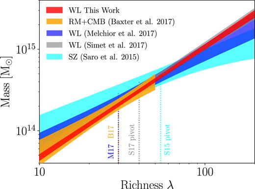
Best fit model for M–λ relation evaluated at the pivot redshift of our model, |$z$|0 = 0.35, compared to other measurements. Our pivot richness is at λ0 = 40. The previous DES result is in blue, from Melchior et al. (2017), while the relation measured in this analysis is in red. The analysis by Baxter et al. (2018) in orange used the same clusters as this work and found a consistent scaling relation over the richness range it probed.
redMaPPer scaling relation comparisons from the literature. Of note, the Simet et al. (2017) results have changed slightly (Simet, private communication). We evaluate log10〈M|λ = 40, |$z$| = 0.35〉 of the other scaling relations in order to compare them to our result, applying the richness correction given by equation (66). When necessary, we use the method presented in Evrard et al. (2014) to convert from richness–mass relations to mass–richness relations. All masses are M200m.
| Authors | Description | log 〈M|λ = 40, |$z$| = 0.35〉 [M⊙] | Richness scaling index Fλ |
|---|---|---|---|
| This work | Weak lensing calibration using DES Y1 | 14.489 ± 0.022 | 1.356 ± 0.052 |
| Melchior et al. (2017) | Weak lensing calibration using DES SV | 14.540 ± 0.067 | 1.12 ± 0.21 |
| Baxter et al. (2018) | CMB lensing calibration using DES Y1 | 14.49 ± 0.31 | 1.24 ± 0.30 |
| Baxter et al. (2016) | Cluster clustering using SDSS | 14.7 ± 0.1 | 1.18 ± 0.16 |
| Simet et al. (2017) | Weak lensing calibration using SDSS | 14.48 ± 0.03 | 1.30 ± 0.09 |
| Murata et al. (2018) | Weak lensing calibration using SDSS | 14.533 ± 0.013 | 1.167 ± 0.052 |
| Farahi et al. (2016) | Pairwise velocity dispersion using SDSS | 14.42 ± 0.10 | 1.31 ± 0.14 |
| Saro et al. (2015) | SZE mass calibration using SPT and DES SV | 14.44 ± 0.05 | 0.91 ± 0.18 |
| Mantz et al. (2016) | Weak lensing of individual WtG clusters | 14.42 ± 0.11 | 1.36 ± 0.21 |
| Geach & Peacock (2017) | CMB lensing calibration using SDSS | 14.37 ± 0.05 | 0.74 ± 0.3 |
Systematic error budget on the amplitude of the mass–richness relation as measured with the DES Y1 data compared to the DES SV result of Melchior et al. (2017). The shear (Section 4.1), photo-|$z$| (Section 4.3), modelling systematics (Section 5.4.1), triaxiality, and projection effects (Section 5.4.2) are conservatively taken to be perfectly correlated between cluster stacks. Membership dilution (Section 4.2) and miscentering (Section 5.2) are assumed to be independent. Statistical and systematic errors are added in quadrature to arrive at the total error.
| Source of systematic | SV Amplitude uncertainty | Y1 Amplitude Uncertainty |
|---|---|---|
| Shear measurement | 4% | 1.7% |
| Photometric redshifts | 3% | 2.6% |
| Modelling systematics | 2% | 0.73% |
| Cluster triaxiality | 2% | 2.0% |
| Line-of-sight projections | 2% | 2.0% |
| Membership dilution + miscentering | ≤1% | 0.78% |
| Total Systematics | 6.1% | 4.3% |
| Total Statistical | 9.4% | 2.4% |
| Total | 11.2% | 5.0% |
Fig. 15 and Table 5 show the mass at λ = 40 and |$z$| = 0.35 as well as the richness scaling index for each of the scaling relations described above.
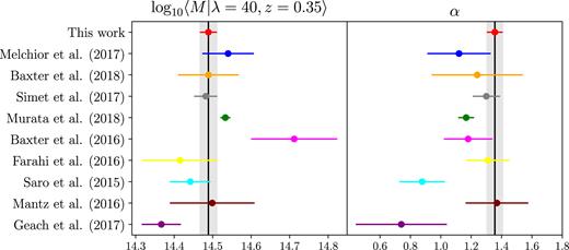
Comparison of the predicted mass at λ = 40 and |$z$| = 0.35 as well as the richness scaling relation between this work (grey bands) and other results from the literature.
8 SYSTEMATIC IMPROVEMENTS FROM DES SV TO DES YEAR 1, AND FROM YEAR 1 TO YEAR 5
Our current analysis has multiple significant improvements relative to Melchior et al. (2017), the precursor to this work. Specifically:
Shear calibration related errors on mass decreased from 4 per cent to 1.7 per cent, based primarily on the data driven correction of shear biases with metacalibration. This implies that the shear calibration uncertainty is no longer the dominant source of systematic error in our weak lensing analysis.
The largest contribution to the systematic uncertainty is now photo-|$z$| errors. In the purely COSMOS-based calibration applied in this work, we find only a minimal improvement between SV and Y1.
The ≈15 per cent increase in uncertainty due to using noisy jackknife estimates of the covariance matrix (Dodelson & Schneider 2013) of the weak lensing profiles was entirely removed through the use of a semi-analytic covariance matrix.
Uncertainty from modelling systematics decreased from 2 per cent to 0.73 per cent. In Melchior et al. (2017), the model calibration corrections were computed by stacking haloes in mass bins. By contrast, our current analysis assigns richness according to a fiducial richness–mass relation, allowing us to stack in richness bins and to therefore accurately compute the correction for a richness bin. Relative to our SV analysis, the amplitude of this correction increased, while its uncertainty was reduced, from 1.00 ± 0.02 to 1.042 ± 0.004. The increase in the correction is primarily due to the richness binning of the haloes as well as the fact that by using the Y1 covariance matrix, the impact of small differences on large scales between our analytical model and numerical simulations is amplified, leading to larger correction factors. More importantly, however, the uncertainty on this correction was greatly reduced. This is due to the semi-analytic covariance matrix as well as allowing for intrinsic scatter of the calibration factors. While we use the semi-analytic covariance matrix for calibration on the simulated profiles, the matrix does not adequately describe the uncertainty in any systematic differences between the model and real data. Additionally, we now fit for the associated systematic uncertainty from the dispersion in the calibration data. Both of these factors result in a decrease in the systematic error budget.
The mass–concentration relation of galaxy clusters is allowed to float in this analysis, while it was held fixed in Melchior et al. (2017). The fixed mass–concentration relation in our SV analysis was necessitated by the relatively low S/N of the weak lensing measurements. By contrast, our current analysis enables us to marginalize over concentration, which in turn should make our results significantly more robust to the impact of baryonic physics in the cores of galaxy clusters (see Section 5.4.1).
All in all, the reduced statistical and systematic uncertainty in our analysis has reduced the error in the amplitude of the mass–richness relation from 11.2 per cent to 5.0 per cent. Unlike our analysis in Melchior et al. (2017), our current constraints are close to systematics limited. Without improved systematics between now and the end of the survey, the improved statistics of the Year 5 data will only decrease our total error budget from 5.0 per cent to ≈4 per cent. Evidently, further reducing systematic uncertainties in future weak lensing mass calibration analysis is imperative.
Photometric redshift errors currently dominate the systematic error budget. Significant improvements in the weak lensing mass calibration of galaxy clusters will require new algorithms for calibrating photometric redshifts. A joint constraint from high-fidelity photo-|$z$|s of matched reference samples and clustering redshifts (Davis et al. 2018; Gatti et al. 2018), as done in Hoyle et al. (2018), is not feasible for higher redshift sources due to the limited redshift range of available spectroscopic or redMaGiC catalogs. Alternatively, source selection criteria that take into consideration photometric redshift uncertainty could lead to a desirable trade off between statistical and systematic uncertainty. With some combination of these approaches, reducing the photometric redshift uncertainty by a factor of two for a year 5 analysis seems plausible.
Related to this, in our current analysis, we have assumed that all systematics are perfectly correlated across all redshift and richness bins. This is likely too conservative. In particular, photometric redshift systematics are unlikely to be perfectly correlated across all redshift bins: the selection of the source population, and their relative signal contribution as a function of source redshift, differ as a function of lens redshift. Adequately characterizing the covariance in the systematic uncertainties associated with photometric redshift errors seems like a relatively simple way to significantly decrease our systematic error budget. For instance, if one were to assume that the photometric redshift systematics were entirely uncorrelated, the associated systematic would be reduced by a factor of |$1/\sqrt{3}$|, rendering photometric redshift errors sub-dominant. This is clearly unrealistic, but it does illustrate that characterizing the covariance in the systematics may lead to significant reductions in the total error budget.
Following photometric redshift uncertainties, three different effects come in at the ≈2 per cent level: shear systematics, triaxiality effects, and projection effects. Of these, shear systematics are the least problematic. We fully expect shear calibration uncertainties will continue to decrease over the coming years, and they will no longer be a major source of error for cluster mass calibration. By contrast, the current systematic error estimates for triaxiality and projection effects clearly demonstrate that there is a significant need for a detailed study of these on weak lensing mass profiles, such as in the recent work of Osato et al. (2018).
Additional, but less urgent, upgrades to our analysis are also possible. For instance, following Murata et al. (2018), an emulator based approach to modelling the halo-matter correlation function or ΔΣ directly can potentially greatly reduce the modelling calibration and its contribution to the uncertainty. Centring errors will also continue to decrease as the availability of multi-wavelength data continues to increase.
Finally, systematics that we have thus far ignored need to be better addressed. For instance, intrinsic alignment by cluster member galaxies even if its effect is very small (Sifón et al. 2015), which impact membership dilution estimates. Likewise, a study of the impact on baryonic physics on our weak lensing calibration methodology is necessary. While we expect these sources of error to be subdominant in our present study, quantifying the systematic error associated with these effects will be increasingly important in the future.
9 SUMMARY AND CONCLUSIONS
We measured the stacked weak lensing signal of redMaPPer clusters in the DES Y1 data. The clusters were divided into 21 subsets of richness and redshift. The mean mass of each cluster stack was estimated for those subsets with λ ≥ 20 and 0.2 ≤ |$z$| ≤ 0.65. Our model incorporated:
Shear measurement systematics (Section 4.1),
Source photometric redshift uncertainties (Section 4.3),
Source sample dilution by cluster members (Section 4.2, Section 5.3.1),
Cluster miscentering (Section 5.2),
Model calibration systematics (Section 5.4),
Triaxiality & projection effects (Section 5.4.2).
The mean masses of the cluster subsets were used to determine the mean cluster mass as a function of richness and redshift according to equation (52). We emphasize that the full analysis was performed blindly: the paper underwent internal review by the DES collaboration prior to unblinding, and no changes to the analysis were made post-unblinding.
The 5.0 per cent constraint on the amplitude of the mass–richness relation is systematics-dominated, with our systematic error alone reaching 4.3 per cent. We stress the systematic uncertainty in the shear and photometric redshift catalogs have been extensively tested and validated, so we are confident our systematic error budget is robust. Halo triaxiality and line of sight projections are now important contributors to the total systematic error, and represent a critical path for minimizing the overall error budget for future analyses
Mass calibration remains the limiting factor for the ability of testing cosmological models with cluster counts. Nevertheless, this work represents a significant step forward: we were able to reduce the systematic error budget from 6.1 per cent in DES Science Verification to 4.3 per cent in DES Year 1. While we will need to achieve similar level of improvements for future analyses including DES Year 5 and LSST Year 1 to significantly improve upon our results, we are confident that we will be able to rise to the challenge: the story of weak lensing mass calibration is one of ever-decreasing systematic errors, a trend that to this day shows no signs of abating.
ACKNOWLEDGEMENTS
This paper has gone through internal review by the DES collaboration. TM and ER are supported by DOE grant DE-SC0015975. TNV and SS are supported by the SFB-Transregio 33 ‘The Dark Universe’ by the Deutsche Forschungsgemeinschaft (DFG) and the DFG cluster of excellence ‘Origin and Structure of the Universe’. ER acknowledges additional support by the Sloan Foundation, grant FG-2016-6443. Support for DG was provided by NASA through Einstein Postdoctoral Fellowship grant number PF5-160138 awarded by the Chandra X-ray Center, which is operated by the Smithsonian Astrophysical Observatory for NASA under contract NAS8-03060. TJ, DH, and SE are supported by DOE grant DE-SC0010107. KR and SB acknowledge support from the UK Science and Technology Facilities Council via Research Training Grants ST/P000252/1 and ST/N504452/1, respectively. CV is supported by the Mexican National Council for Science and Technology via grant number 411117. AvdL is supported by DoE grant DE-SC0018053.
Part of our computations have been carried out on the computing facilities of the Computational Center for Particle and Astrophysics (C2PAP). A portion of this research was carried out at the Jet Propulsion Laboratory, California Institute of Technology, under a contract with the National Aeronautics and Space Administration.
Funding for the DES Projects has been provided by the U.S. Department of Energy, the U.S. National Science Foundation, the Ministry of Science and Education of Spain, the Science and Technology Facilities Council of the United Kingdom, the Higher Education Funding Council for England, the National Center for Supercomputing Applications at the University of Illinois at Urbana-Champaign, the Kavli Institute of Cosmological Physics at the University of Chicago, the Center for Cosmology and Astro-Particle Physics at the Ohio State University, the Mitchell Institute for Fundamental Physics and Astronomy at Texas A&M University, Financiadora de Estudos e Projetos, Fundação Carlos Chagas Filho de Amparo à Pesquisa do Estado do Rio de Janeiro, Conselho Nacional de Desenvolvimento Científico e Tecnológico and the Ministério da Ciência, Tecnologia e Inovação, the Deutsche Forschungsgemeinschaft and the Collaborating Institutions in the Dark Energy Survey.
The Collaborating Institutions are Argonne National Laboratory, the University of California at Santa Cruz, the University of Cambridge, Centro de Investigaciones Energéticas, Medioambientales y Tecnológicas-Madrid, the University of Chicago, University College London, the DES-Brazil Consortium, the University of Edinburgh, the Eidgenössische Technische Hochschule (ETH) Zürich, Fermi National Accelerator Laboratory, the University of Illinois at Urbana-Champaign, the Institut de Ciències de l’Espai (IEEC/CSIC), the Institut de Física d’Altes Energies, Lawrence Berkeley National Laboratory, the Ludwig-Maximilians Universität München and the associated Excellence Cluster Universe, the University of Michigan, the National Optical Astronomy Observatory, the University of Nottingham, The Ohio State University, the University of Pennsylvania, the University of Portsmouth, SLAC National Accelerator Laboratory, Stanford University, the University of Sussex, Texas A&M University, and the OzDES Membership Consortium.
Based in part on observations at Cerro Tololo Inter-American Observatory, National Optical Astronomy Observatory, which is operated by the Association of Universities for Research in Astronomy (AURA) under a cooperative agreement with the National Science Foundation.
The DES data management system is supported by the National Science Foundation under Grant Numbers AST-1138766 and AST-1536171. The DES participants from Spanish institutions are partially supported by MINECO under grants AYA2015-71825, ESP2015-66861, FPA2015-68048, SEV-2016-0588, SEV-2016-0597, and MDM-2015-0509, some of which include ERDF funds from the European Union. IFAE is partially funded by the CERCA program of the Generalitat de Catalunya. Research leading to these results has received funding from the European Research Council under the European Union’s Seventh Framework Program (FP7/2007-2013) including ERC grant agreements 240672, 291329, and 306478. We acknowledge support from the Australian Research Council Centre of Excellence for All-sky Astrophysics (CAASTRO), through project number CE110001020, and the Brazilian Instituto Nacional de Ciência e Tecnologia (INCT) e-Universe (CNPq grant 465376/2014-2).
This manuscript has been authored by Fermi Research Alliance, LLC under Contract No. DE-AC02-07CH11359 with the U.S. Department of Energy, Office of Science, Office of High Energy Physics. The United States Government retains and the publisher, by accepting the article for publication, acknowledges that the United States Government retains a non-exclusive, paid-up, irrevocable, world-wide license to publish or reproduce the published form of this manuscript, or allow others to do so, for United States Government purposes.
This work used simulations and computations performed using computational resources at SLAC and at NERSC.
Footnotes
This correction is also referred to as a boost factor as the measured signal should be boosted to correct for the contamination.
REFERENCES
APPENDIX A: The redMaPPer v6.4.17 Cluster Catalog
The full redMaPPer DES Y1A1 catalogues will be available at http://risa.stanford.edu/redmapper/ in FITS format. The catalogs will also be available from the online journal in machine-readable formats. We note that this is of the same format as Rykoff et al. (2016), and we point the reader to that paper for further details. The cluster catalogue is described in Table A1, and the associated members in Table A2. The catalogue is the ‘full’ catalogue, with all clusters with λ > 20, and the volume-limited subset is flagged with the VLIM flag. The map of the maximum redshift of the volume-limited catalogue is described in Table A3, and the random points are described in Table A4.
redMaPPer Y1A1 cluster catalog format.
| Name | Format | Description |
|---|---|---|
| ID | INT(4) | redMaPPer Cluster Identification Number |
| VLIM | INT(2) | One if in cosmology catalog, 0 otherwise |
| NAME | CHAR(20) | redMaPPer Cluster Name |
| RA | FLOAT(8) | Right ascension in decimal degrees (J2000) |
| DEC | FLOAT(8) | Declination in decimal degrees (J2000) |
| Z_LAMBDA | FLOAT(4) | Cluster photo-|$z$||$z$|λ |
| Z_LAMBDA_ERR | FLOAT(4) | Gaussian error estimate for |$z$|λ |
| LAMBDA | FLOAT(4) | Richness estimate λ |
| LAMBDA_ERR | FLOAT(4) | Gaussian error estimate for |$z$|λ |
| S | FLOAT(4) | Richness scale factor |
| Z_SPEC | FLOAT(4) | Spectroscopic redshift for most likely center (-1.0 if not available) |
| COADD_OBJECTS_ID | INT(8) | DES COADD_OBJECTS_ID identification number |
| MAG_CM_G | FLOAT(4) | g MAG_CM magnitude for most likely central galaxy (SLR corrected) |
| MAGERR_CM_G | FLOAT(4) | error on g MAG_CM magnitude |
| MAG_CM_R | FLOAT(4) | r MAG_CM magnitude for most likely central galaxy (SLR corrected) |
| MAGERR_CM_R | FLOAT(4) | error on g MAG_CM magnitude |
| MAG_CM_I | FLOAT(4) | i MAG_CM magnitude for most likely central galaxy (SLR corrected) |
| MAGERR_CM_I | FLOAT(4) | error on g MAG_CM magnitude |
| MAG_CM_Z | FLOAT(4) | |$z$| MAG_CM magnitude for most likely central galaxy (SLR corrected) |
| MAGERR_CM_Z | FLOAT(4) | error on g MAG_CM magnitude |
| ZLUM | FLOAT(4) | Total membership-weighted |$z$|-band luminosity (units of L*) |
| P_CEN[5] | 5×FLOAT(4) | Centering probability Pcen for 5 most likely centrals |
| RA_CEN[5] | 5×FLOAT(8) | R.A. for 5 most likely centrals |
| DEC_CEN[5] | 5×FLOAT(8) | Decl. for 5 most likely centrals |
| ID_CEN[5] | 5×INT(8) | DES COADD_OBJECTS_ID identification number for 5 most likely centrals |
| PZBINS[21] | 21×FLOAT(4) | Redshift points at which P(|$z$|) is evaluated |
| PZ[21] | 21×FLOAT(4) | P(|$z$|) evaluated at redshift points given by PZBINS |
redMaPPer DES Y1A1 member catalog format.
| Name | Format | Description |
|---|---|---|
| ID | INT(4) | redMaPPer Cluster Identification Number |
| RA | FLOAT(8) | Right ascension in decimal degrees (J2000) |
| DEC | FLOAT(8) | Declination in decimal degrees (J2000) |
| R | FLOAT(4) | Distance from cluster center (|$h^{-1}\, \mathrm{Mpc}$|) |
| P | FLOAT(4) | Membership probability |
| P_FREE | FLOAT(4) | Probability that member is not a member of a higher ranked cluster |
| THETA_L | FLOAT(4) | Luminosity (|$z$|-band) weight |
| THETA_R | FLOAT(4) | Radial weight |
| MAG_CM_G | FLOAT(4) | g MAG_CM magnitude (SLR corrected) |
| MAGERR_CM_G | FLOAT(4) | error on g MAG_CM magnitude |
| MAG_CM_R | FLOAT(4) | r MAG_CM magnitude (SLR corrected) |
| MAGERR_CM_R | FLOAT(4) | error on r MAG_CM magnitude |
| MAG_CM_I | FLOAT(4) | i MAG_CM magnitude (SLR corrected) |
| MAGERR_CM_I | FLOAT(4) | error on i MAG_CM magnitude |
| MAG_CM_Z | FLOAT(4) | |$z$| MAG_CM magnitude (SLR corrected) |
| MAGERR_CM_Z | FLOAT(4) | error on |$z$| MAG_CM magnitude |
| Z_SPEC | FLOAT(4) | Spectroscopic redshift (-1.0 if not available) |
| COADD_OBJECTS_ID | INT(8) | DES COADD_OBJECTS_ID identification number |
redMaPPer |$z$|max map format.
| Name | Format | Description |
|---|---|---|
| HPIX | INT(8) | HEALPIX ring-ordered pixel number (NSIDE = 4096) |
| ZMAX | FLOAT(4) | Maximum redshift of a cluster centered in this pixel |
| FRACGOOD | FLOAT(4) | Fraction f pixel area that is not masked |
| Name | Format | Description |
|---|---|---|
| HPIX | INT(8) | HEALPIX ring-ordered pixel number (NSIDE = 4096) |
| ZMAX | FLOAT(4) | Maximum redshift of a cluster centered in this pixel |
| FRACGOOD | FLOAT(4) | Fraction f pixel area that is not masked |
redMaPPer random points catalogue format.
| Name | Format | Description |
|---|---|---|
| RA | FLOAT(8) | Right ascension in decimal degrees (J2000) |
| DEC | FLOAT(8) | Declination in decimal degrees (J2000) |
| Z | FLOAT(4) | Redshift of random point |
| LAMBDA | FLOAT(4) | Richness of random point |
| WEIGHT | FLOAT(4) | Weight of random point |
APPENDIX B: PARAMETER POSTERIORS
When fitting the weak lensing profiles, some parameters are not constrained by a prior and are also not shared between cluster bins. These are the halo concentration c, the boost factor amplitude B0, and the boost factor scale radius Rs. Table B1 shows the posteriors for these three parameters for each cluster bin. As seen in Fig. 10B0 and Rs are highly degenerate.
Lensing profile parameters not constrained by priors or shared between cluster bins. Uncertainties are the 68 per cent confidence intervals. Note that in the highest redshift and richness bin, the boost factor profile model scale radius had a bimodal distribution, and is not well constrained. This did not affect the mass estimate at all.
| λ | |$z$| ∈ [0.2, 0.35) | |$z$| ∈ [0.35, 0.5) | |$z$| ∈ [0.5, 0.65) |
|---|---|---|---|
| Concentration c | |||
| [20, 30) | 5.81 ± 1.03 | 5.68 ± 1.14 | 4.76 ± 1.62 |
| [30, 45) | 4.53 ± 0.74 | 6.24 ± 1.08 | 3.61 ± 0.72 |
| [45, 60) | 4.38 ± 0.96 | 5.41 ± 1.17 | 4.76 ± 1.21 |
| [60, ∞) | 4.65 ± 0.82 | 3.19 ± 0.56 | 3.73 ± 1.02 |
| Boost factor amplitude B0 | |||
| [20, 30) | 0.34 ± 0.05 | 0.05 ± 0.01 | 0.13 ± 0.05 |
| [30, 45) | 0.37 ± 0.06 | 0.14 ± 0.04 | 0.13 ± 0.08 |
| [45, 60) | 0.27 ± 0.05 | 0.05 ± 0.02 | 0.09 ± 0.06 |
| [60, ∞) | 0.23 ± 0.03 | 0.21 ± 0.17 | 0.03 ± 0.04 |
| Boost factor scale radius Rs [Mpc] | |||
| [20, 30) | 0.44 ± 0.06 | 0.89 ± 0.24 | 0.38 ± 0.11 |
| [30, 45) | 0.50 ± 0.07 | 0.44 ± 0.10 | 0.44 ± 0.18 |
| [45, 60) | 0.80 ± 0.15 | 1.72 ± 0.95 | 0.85 ± 0.37 |
| [60, ∞) | 1.37 ± 0.21 | 0.51 ± 0.23 | 35.94 ± 29.69 |
Author notes
Einstein Fellow.
