


ABSTRACT
We investigate star-galaxy classification for astronomical surveys in the context of four methods enabling the interpretation of black-box machine learning systems. The first explores the decision boundaries as given by decision tree based methods, enabling the visualization of the classification categories. Secondly, we investigate how the Mutual Information based Transductive Feature Selection (MINT) algorithm can be used to perform feature preselection. If a small number of input features is required for the machine learning classification algorithm, feature preselection provides a method to determine which of the many possible input features should be selected. Third is the use of the tree-interpreter package to enable popular decision tree based ensemble methods to be opened, visualized, and understood. This is done by additional analysis of the tree-based model, determining not only which features are important to the model, but how important a feature is for a particular classification given its value. Lastly, we use decision boundaries from the model to revise an already existing method of classification, essentially asking the tree-based method where decision boundaries are best placed and defining a new classification method. We showcase these techniques by applying them to the problem of star-galaxy separation using data from the Sloan Digital Sky Survey (hereafter SDSS). We use the output of MINT and the ensemble methods to demonstrate how more complex decision boundaries improve star-galaxy classification accuracy over the standard SDSS frames approach (reducing misclassifications by up to |${\approx }33{{\ \rm per\ cent}}$|).
1 INTRODUCTION
An important and long-standing problem in astronomy is that of object classification; for example, whether an object in a photographic plate is a nearby star or a distant galaxy. Independent of the data sample under investigation, the process of building a source catalogue will require object classification. There are multiple ways of determining the classification of astronomical objects, each with their own advantages and disadvantages. For example, template fitting methods applied to photometric (Baum 1962; Puschell, Owen & Laing 1982) or spectroscopic data (Cappellari & Emsellem 2004; Sarzi et al. 2006) can be accurate but are dependent on the choice of templates, whereas classifying objects by radial profile (Le Fevre et al. 1986) can be quick, but of limited accuracy due to the small amount of information used for each object. For instance, radial profile data alone cannot be used to distinguish between point sources, such as stars and quasars (QSOs).
There are successful complex point source separation methods in use to identify astronomical objects, such as likelihood functions (Kirkpatrick et al. 2011), where an object is classified as a QSO based on the summed Gaussian distance to every object in a set of known QSOs and stars in colour space. There are also complex machine learning methods for object classification that exist, such as Artificial Neural Networks that use photometry to isolate high-redshift QSOs (Yèche et al. 2010), or objects at fainter magnitudes (Soumagnac et al. 2015). A comparison of many of these methods applied to Dark Energy Survey Y1 data can be found in Sevilla-Noarbe et al. (2018).
This paper aims to introduce a new combination of machine learning data analysis methods to astronomy,1 specifically in the case of object classification, although we note that these methods can be readily applied to other problems. The goal is to use machine learning to improve the precision/purity of object classification from photometric data, while simultaneously analysing the generated machine learning models in an effort to understand the decision-making processes involved. The object classification method we aim to improve on is the classification parameter stored in the Sloan Digital Sky Survey (SDSS) catalogue as frames.
We achieve this by selecting data properties relevant to the classification problem, then using those data with a range of machine learning algorithms to classify astronomical objects. During object classification, information behind the decision-making process that is usually internal to the machine learning algorithm will be gathered, output, and visualized to achieve a deeper understanding of how the machine learning algorithm succeeds in classifying individual objects.
The paper is laid out as follows: Section 2 describes the SDSS data and standard classification method behind assigning the frames parameter, Section 3 describes the new methods employed in this work, including feature selection, a comparison of algorithm performance, and methods to interpret the decision-making processes in one of the tree-based algorithms. Section 4 details the results obtained from these methods in terms of purity and completeness. In Section 5, we discuss the results and conclude.
2 DATA
In this section we introduce the observational data used in this paper, which is drawn from the SDSS (Gunn et al. 1998). We briefly review the standard photometric star/galaxy classification criterion given by the frames method which is obtained through the query of the objc_type parameter (Stoughton et al. 2002) in the CasJobs SkyServer (Szalay et al. 2002).
2.1 Observational data
The data in this work are drawn from SDSS Data Release 12 (DR12, Alam et al. 2015). The SDSS uses a 2.5 m telescope at Apache Point Observatory in New Mexico and has CCD wide field photometry in five bands (u, g, r, i, |$z$|, York et al. 2000; Smith et al. 2002; Gunn et al. 2006; Doi et al. 2010), including an expansive spectroscopic follow-up program (Eisenstein et al. 2011; Dawson et al. 2013; Smee et al. 2013) covering 14 555 square degrees of the northern and equatorial sky. The SDSS collaboration has obtained more than three million spectra of astronomical objects using dual fiber-fed spectrographs. An automated photometric pipeline performs object classification to an r band magnitude of r ≈ 22 and measures photometric properties of more than 100 million galaxies. The complete data sample, and many derived catalogues including galaxy photometric properties, are publicly available through the CasJobs server (Li & Thakar 2008).2
As we will draw large random samples from the SDSS DR12 data, we first obtain the full relevant data set. We obtain object IDs, magnitudes, and errors as measured in different apertures in each band, radial profiles, both photometric and spectroscopic type classifications, and photometry quality ‘flags’ using the query submitted to CasJobs shown in Appendix A. Flags are useful indicators of the status of each object in the catalogue, and warn of possible problems with the object images, or possible problems with the various measurements related to the object.3 The resulting catalogue is similar to that used in Hoyle et al. (2015), but we omit redshift information. We generate a range of standard colours (e.g. PSFMAG_U-PSFMAG_G) and non-standard colours (e.g. PSFMAG_U-CMODELMAG_G) for each object. The final catalogue contains 215 input quantities, or ‘features’. The magnitudes used in this work are corrected for galactic extinction where appropriate. We further filter objects that have a clean spectroscopic classification by selecting objects with a Zwarning flag in the catalogue that is equal to zero. This selection removes |${\approx }11{{\ \rm per\ cent}}$| of the sample.
The final catalogue contains 3751 496 objects. We note that approximately 66 per cent of these objects are spectroscopically classified as galaxies with the remaining objects classified as point sources. We select two random samples from the final catalogue: the first is a training sample of 10 000 objects and the second is a test sample comprised of 1.5 million objects. The small training sample allows a large exploration of model space to be completed in a tractable time-scale.
2.2 Existing SDSS classification schemes: spectral fitting and photometric selection
The SDSS provides both a spectroscopic and a photometric classification for each object which both attempt to infer if the object is a galaxy or a point source, including both stars and QSOs. We briefly review both techniques below.
The spectroscopic classification is stored in a catalogue parameter called CLASS, which is assigned by comparing spectral templates and the observed spectra using a χ2 cost function (Bolton et al. 2012). During this process galaxy templates are restricted in the redshift range, 0 < |$z$| < 2 and QSO templates are restricted to |$z$| < 7. We note that the observed spectra are masked outside the wavelength range of 3600 Å–10 400 Å. This paper assumes that this analysis produces the true object classification due to the fact that this method directly determines the differences between single stellar spectra and compound galaxy spectra of many stars, and we will use it to compare different photometric classification predictions.
A second empirical method using photometric data is called frames (stored as the objc_type parameter in the CasJobs SkyServer), and uses the combination of following photometric magnitude measurements PSFMAG-X - CMODELMAG-X. The PSFMAG magnitude is calculated by fitting a point spread function model to the object which is then aperture corrected, as appropriate for isolated stars and point sources (see Stoughton et al. 2002). The CMODELMAG magnitude is a composite measurement generated by a linear combination of the best-fitting exponential and de Vaucouleurs light profile fits in each band. The resulting CMODELMAG magnitude is in excellent agreement with Petrosian magnitudes for galaxies, and PSF magnitudes of stars (Abazajian et al. 2004). Therefore the condition PSFMAG-X - CMODELMAG-X is a reasonable discriminator between galaxies and point sources.
The SDSS pipeline provides the frames classification for each object in each photometric band, as well as an overall classification calculated by summing the fluxes in all bands and applying the same criterion as in equation (1). We use this latter summation as the base-line SDSS photometric classification scheme in this work. It is our understanding that this threshold of 0.145 was chosen through experimentation, as discussed in section 4.4.6.1 of Stoughton et al. (2002).
We show the distribution in PSFMAG versus CMODELMAG for the training sample in Fig. 1, with the condition given in equation (1) as the dashed black line, and the colours denoting spectroscopic classification.
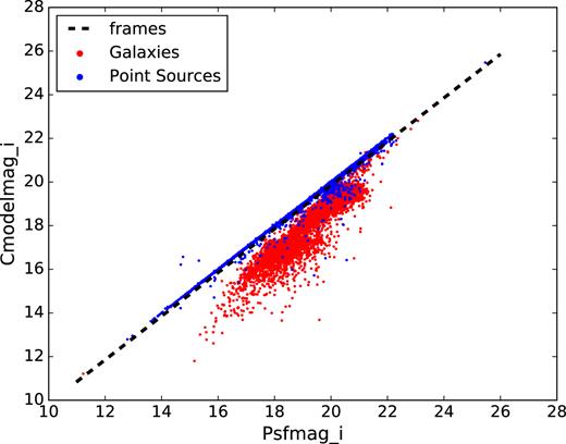
Object classification using the frames method. Here we show two magnitude estimates in the I band of the training sample, with the discriminating dashed black line drawn according to equation (1), and the colours denoting spectroscopic classification.
In this paper, we investigate if a new photometric classification can improve the accuracy of the frames methods, and if by understanding how some machine learning systems work, we can motivate changes to these base-line photometric classification schemes. The authors of the frames method state that it accurately classifies objects at the 95 per cent confidence level to r =21, and that the method becomes unreliable at fainter magnitudes (Stoughton et al. 2002).
2.3 Data preparation
For the main body of this work, we only select data with good photometry and spectra. In particular, we select objects in the catalogue where their clean flag is equal to one. This removes objects which are duplicates, or with deblending issues, interpolation issues, or have suspicious detections, or are stars close to the edge of the survey.
We explore how this may bias our results, and perform a stand-alone test in Section 4.1 with and without the clean flag selection to determine what effect this has on our accuracy.
3 METHODS
This section introduces the machine learning algorithms used in this work, including the methodologies behind the MINT feature selection algorithm (He et al. 2015) and a method to simplify ensemble methods based on decision trees called treeinterpreter (Saabas 2015). We also describe how machine learning algorithms can be used to motivate improvements to the base-line SDSS frames classification.
3.1 Object classification using machine learning methods
Four tree-based machine learning methods are used in this work: Random Forest (RF, Breiman 2001), Adaboost (ADA, Freund & Schapire 1997; Zou et al. 2009), Extra Randomized Trees (EXT, Geurts, Ernst & Wehenkel 2006), and Gradient Boosted Trees (GBT, Friedman 1999, 2001; Hastie, Tibshirani & Friedman 2009). We use the implementations of these algorithms from within the scikit-learn python package (Pedregosa et al. 2011) – tools for data mining and data analysis. All of these methods are able to draw a decision boundary in multidimensional parameter spaces which distinguishes classification classes. We describe these algorithms briefly below.
A decision tree is a flowchart-like model that makes ever finer partitions of the input features (here photometric properties) of the training data. Each partition is represented by a branch of the tree. The input feature and feature value used to generate the partitions are chosen to maximize the success rate of the target values (here point source or galaxy classifications) which reside on each branch. This process ends at leaf nodes, upon which one or more of the data sit. A new object is queried down the tree and lands on a final leaf node. It is assigned a predicted target value from the true target values of the training data on the leaf node. A single decision tree is very prone to over fitting training data.
Random Forests train by generating a large number of decision trees, with each tree using a bootstrap resample of the training data and a random sample of the input features. During classification of new data the majority vote across all trees is taken. By building a model that takes a vote from many decision trees, the problem of over fitting the training set is overcome, allowing better generalization to unseen data.
Extra Randomized Trees is a similar algorithm to Random Forests, but splits in the generated decision trees are decided at random instead of calculating a metric. This makes model training faster and can further improve generalization.
Adaboost and Gradient Boosted Trees are both examples of boosted algorithms, which convert so-called decision stumps into strong learners. Decision stumps are shallow decision trees (trees with a low depth) that result in predictions close to a random guess. The data are processed through these trees multiple times with the algorithm weighting the model based on performance. Adaboost changes the model between iterations by re-weighting the data of objects that were misclassified at a rate governed by the learning_rate parameter. This minimizes model error by focusing the subsequent tree on those misclassified objects. Gradient Boosted Trees changes the model by iteratively adding decision stumps according to the minimization of a differentiable loss function (which tracks misclassification) using gradient descent. The model will start with an ensemble of decision stumps and the loss will be assessed. Between each iteration the algorithm adds decision stumps that reduce the loss of the model, stopping when loss can no longer be reduced (when the gradient of reducing loss flattens).
In this paper, we will perform object classification using each of these four algorithms, for each of the following three subsets of photometric features:
the five features that the SDSS pipeline uses in the frames method (i.e. PSFMAG – CMODELMAG for each filter);
five features selected using a feature selection method, MINT as discussed in Section 3.2;
all 215 features available in the sample.
Each test is performed with 10 000 objects in the training sample, predicting on a test sample of 1.5 million objects. We will show the results for accuracy of classification in Section 4.2 for each algorithm (Random Forests, Extra Randomized Trees, Gradient Boosted Trees, and Adaboost), operating on the different subsets of photometric features. In this work, accuracy of classification is 100 per cent when the classification provided from the tree-based algorithms or the frames method is equal to the classification provided by the CLASS parameter.
| True Galaxies | True Point Sources | |
|---|---|---|
| Objects classified as galaxies | Tg | Fps |
| Objects classified as point sources | Fg | Tps |
| True Galaxies | True Point Sources | |
|---|---|---|
| Objects classified as galaxies | Tg | Fps |
| Objects classified as point sources | Fg | Tps |
| True Galaxies | True Point Sources | |
|---|---|---|
| Objects classified as galaxies | Tg | Fps |
| Objects classified as point sources | Fg | Tps |
| True Galaxies | True Point Sources | |
|---|---|---|
| Objects classified as galaxies | Tg | Fps |
| Objects classified as point sources | Fg | Tps |
Fig. 2 shows an example of the decision boundaries created from a Random Forest run using only two features, a simplified version of the first test in the list above. The area where the algorithm classifies objects as galaxies is shown in red, with classifications of stars shown in blue. The areas where classifications are more distinct have bolder colours, with the area around the horizontal boundary showing more uncertainty in object classification. The plotted points show all 10 000 objects of the training sample, colour coded by their spectroscopic type. It should be noted that the Random Forest draws boundaries very similar to the ones in the SDSS pipeline paper, though not as linear. However, it can be seen that some objects are misclassified using both the frames method and this particular Random Forest run. Using more than two features, such as in the tests listed above, allows the machine learning methods to utilize more dimensions in parameter space and consequently achieve a higher accuracy of classification.
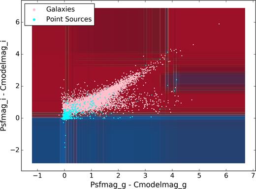
Training data (pink and cyan points for galaxies and point sources) plotted over the decision boundaries (red and blue background for galaxies and point sources), generated by an example Random Forest run using frames features in g and i band. The colour of the training data denotes spectroscopic classification.
3.2 Feature selection using MINT
The SDSS pipeline measures and calculates a rich abundance of features from the photometric images. Rather than just focusing on those features employed in the frames algorithm, one may also choose other available features to pass to the machine learning algorithms. To aid in the interpretation of the results it would be advantageous to select only a small number of features, but chosen wisely such that they are minimally correlated with each other, and have strong classifying power (Andrew. Hall 2000). Various feature selection methods have been explored in recent years in relation to object classification problems, such as the Fisher discriminant (A. A.; Soumagnac et al. 2015), or the previously mentioned feature_importance function provided in the scikit-learn package (Pedregosa et al. 2011; Hoyle et al. 2015).
Another suitable method of feature selection is ‘Maximum Relevance and Minimum Redundancy’ (mRMR) which can help to find a small number of relevant input features without relinquishing classification power. This has been proven to work in multiple data sets involving handwritten digits, arrhythmia, NCI cancer cell lines, and lymphoma tissues (Ding & Peng 2005; Peng, Long & Ding 2005).
This work uses an extension of mRMR called Mutual Information based Transductive Feature Selection (MINT) (He et al. 2015), a method designed to help with the ‘curse of dimensionality’ in genome trait prediction. This arises due to the issue of having many more features than samples in the data set. MINT assesses the mutual information between the training sample’s features and classification and, setting it apart from mRMR, between individual features in both the training and test sample.
This means that MINT can effectively combine equations (4) and (5) into equation (6), the same as mRMR, but is able to exploit a much larger amount of data due to the assessment of the correlation between features for the entire sample, not just the training sample. For this work, MINT is able to utilize photometric data from the 1.5 million objects in the test sample. This allows us to ensure, much more than we could using mRMR alone, that the selected features will be those which are correlated least with one another, thus giving us the best chance of accurate object classification.
We follow He et al. (2015) and explore the high-dimensional feature space using the greedy algorithm (Vince 2002). In the case of MINT, greedy means that parts of the calculation are performed dynamically – utilizing previously calculated values in the MINT algorithm for future MINT calculations – making the feature selection process vastly quicker.
A user-defined number of features is selected using the MINT algorithm, thus reducing the amount of input data (by reducing the number of features) required to make a robust prediction for the test sample. In this work, we reduce the number of features from 215 to five using MINT. This is to mirror the number of features the frames method uses and to test whether we can make accurate predictions with severely reduced data per object.
Table 2 shows the results of the MINT feature selection method for five or 10 total selected features. It can be seen that there are features in common between these two sets; these have clearly been identified as robust and distinct features for classification.
The features selected by MINT when setting the total number of features to five, or 10. PSFMAG, DERED, FIBERMAG, and CMODELMAG are all different estimates of magnitude in the five possible SDSS bands of u, g, r, i, and |$z$|.
| Number of selected MINT features (using 10 000 training objects and 1.5 million test objects) | |
|---|---|
| 5 | 10 |
| PSFMAG_G - CMODELMAG_R | DERED_Z - FIBERMAG_R |
| PSFMAG_I - FIBERMAG_I | PSFMAG_I - CMODELMAG_I |
| DERED_G - FIBERMAG_G | PSFMAG_I - FIBERMAG_I |
| PSFMAG_I - CMODELMAG_I | DERED_G - FIBERMAG_G |
| PSFMAG_R - FIBERMAG_Z | PSFMAG_G - CMODELMAG_R |
| PSFMAG_Z - FIBERMAG_Z | |
| PSFMAG_G - CMODELMAG_G | |
| PSFMAG_R - FIBERMAG_Z | |
| DERED_R - PSFMAG_R | |
| PSFMAG_R - FIBERMAG_R | |
We investigated the effect of changing the number of MINT-selected features on the classification accuracy in a test Random Forest run (with 256 trees and no set maximum depth). This can be seen in Fig. 3. The accuracy of the results only increases slightly (≈0.2 per cent) as the number of MINT-selected features increases. Also shown is the effect of changing the number of objects in the training sample. Again, the accuracy does not change significantly (<1 per cent).
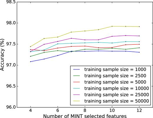
Effect of number of MINT-selected features on predictive accuracy. Coloured lines denote the number of objects used in the training sample.
3.3 Interpreting models of tree-based methods
We use tree-based machine learning methods because they are robust, difficult to overfit, and have methods available to aid in interpreting them (Hastie et al. 2009). By examining the decision trees created by the algorithm, the inner workings of the model can be understood. However, when the data are vast and complex and an ensemble of trees is used, the scope of the model deepens to such a degree that interpretation becomes nearly impossible. It is for this reason that new methods of model interpretation must be investigated.
An example decision tree taken from a Random Forest comprised of 256 trees and no limit on the hyperparameter ‘maximum depth’, can be seen in Fig. 4. In this work, an example of how a node splits data (an example question in the decision tree) would be PSFMAG_R - CMODELMAG_R ≤ 0.25. Depending on the answer to this question, the object would advance through the tree in one direction or another towards the leaves (predicted class). It is clear from the complexity of the tree that it is unfeasible to easily gain information relating to the inner workings of the model by simply looking through the trees. This is especially the case since each tree will have drawn different decision boundaries relating to specific types of objects. For example, one tree may be very good at classifying red point sources, while another may excel at classifying blue galaxies.
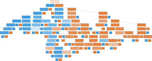
Example of a single decision tree from a Random Forest comprised of 256 trees with unrestricted maximum depth. The blue colours indicate a point source classification, while orange colours indicate a galaxy classification. Opacity of colour represents probability of classification with more solid colours denoting higher probabilities.
There are methods for determining which features are important to the machine learning model, such as the feature_importance function provided in the scikit-learn package (Pedregosa et al. 2011). This is sometimes referred to as the ‘mean decrease impurity’, which is the total decrease in node impurity, an assessment of how well the model is splitting the data, averaged over all of the trees in the ensemble (Breiman et al. 1984). This is to say that the features in the model are assessed, and if they consistently contribute to making classifications, their importance increases. This is useful, but somewhat ambiguous as it does not give much insight into the individual decisions the trees make, such as where it is most efficient to draw a boundary in parameter space.
Instead, a python package called treeinterpreter4 (Saabas 2015) can be used in an effort to decipher this information. For each object, treeinterpreter follows the path through the tree, taking note of the value of the feature in question every time it contributes or detracts from an object being given a particular classification. This means that one can investigate how much the value of a particular feature contributes to the probability of a certain classification.
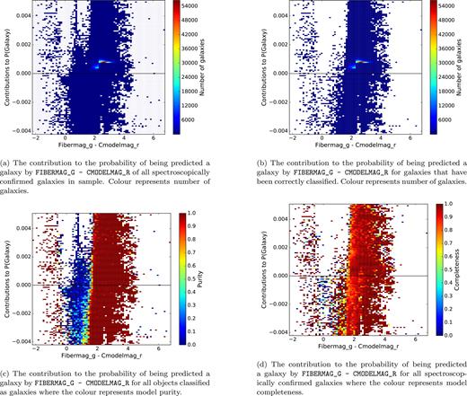
Density plot of contributions to the probability of a galaxy classification by PSFMAG_G - CMODELMAG_I for spectroscopically confirmed galaxies. Purity refers to the fraction of retrieved instances that are relevant; completeness is the fraction of relevant instances that are retrieved. In relation to this work, purity would be a measure of how many galaxy classifications correctly identified galaxies, and completeness would be a measure of how many galaxies were correctly identified out of the total number of galaxies. This example was created with a Random Forest comprising of 256 trees with no maximum depth, using all 215 available features. (a) The contribution to the probability of being predicted a galaxy by FIBERMAG_G - CMODELMAG_R of all spectroscopically confirmed galaxies in sample. Colour represents number of galaxies. (b) The contribution to the probability of being predicted a galaxy by FIBERMAG_G - CMODELMAG_R for galaxies that have been correctly classified. Colour represents number of galaxies. (c) The contribution to the probability of being predicted a galaxy by FIBERMAG_G - CMODELMAG_R for all objects classified as galaxies where the colour represents model purity. (d) The contribution to the probability of being predicted a galaxy by FIBERMAG_G - CMODELMAG_R for all spectroscopically confirmed galaxies where the colour represents model completeness.
Fig. 5(a) shows the contribution to the probability of galaxy classification from FIBERMAG_G - CMODELMAG_R, for all of the galaxies in the test sample, given a Random Forest model trained on 10 000 objects (using 256 trees and all 215 features in our catalogue). The colours show the number of objects with white showing the absence of data. Most of the galaxies fall into a small line of assigned probability of 0.002 at a FIBERMAG_G - CMODELMAG_R value of approximately 2.3, the mean of the sample, with the remaining galaxies scattered around the plot making up the blue colour. For this particular feature, FIBERMAG_G - CMODELMAG_R, some objects in the sample are given a reduced probability of being galaxies (i.e. they receive a negative contribution to probability); these are the data points below the black line. The model does not necessarily incorrectly classify these galaxies due to this one feature; there may be other features that are more important to the model than this one for classifying these particular galaxies.
Fig. 5(b) shows the same as 5(a), but for all the galaxies in the test sample that were correctly classified as galaxies. The colouring is the same as in Fig. 5(a). There are a number of galaxies with a FIBERMAG_G - CMODELMAG_R value of zero to two that were incorrectly classified as point sources by the model, as they are missing when comparing to Fig. 5(a).
The colour of Fig. 5(c) shows the purity of the galaxy classification, the fraction of retrieved instances that are relevant. Here it can be seen that the model has failed to correctly classify bluer galaxies, where FIBERMAG_G - CMODELMAG_R is closer to zero. This is because that region of parameter space is being used to classify point sources, see Fig. 6.
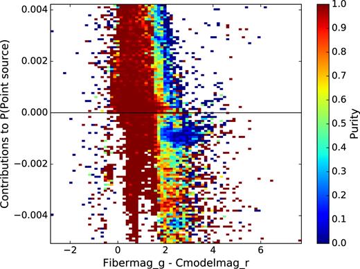
The contribution to the probability of being classified as a point source by FIBERMAG_G - CMODELMAG_R where the colour represents purity. The correctly classified point sources here are occupying the parameter space of the incorrectly classified galaxies in Fig. 5(c).
The colour of Fig. 5(d) shows the completeness of the galaxy classification; this can be interpreted as the probability that the object will be a galaxy given the model. Around values of FIBERMAG_G - CMODELMAG_R= 0, it can be seen that the model begins to fail at classifying galaxies correctly.
Visual analysis of this kind provides insight into how the model is drawing boundaries in parameter space, and information about where the limitations of the classifications arise.
3.4 Performance of algorithms
Each machine learning method used in this work was tuned to optimize classification performance. This is achieved by varying the hyperparameters for each algorithm (such as number of trees and tree depth) and assessing the performance of the model using k-fold cross-validation (Mosteller & Tukey 1968). The scikit-learn implementation of this method is called GridsearchCV.5 In the K-fold cross-validation method, the best hyperparameters are determined by splitting the training data up into a user-defined number of groups (10 for example), training the model on nine of the groups, and testing the model on the last remaining group. The groups are then rotated until each group has been tested and the results of the tests are averaged. This process is performed for each set of hyperparameters, the results from the averaged tests are compared, and the set of hyperparameters with the best results is chosen.
The explored hyperparameters are: n_estimators: the number of trees, max_features: the number of features to consider when looking for the best split within a tree, min_samples_leaf: the minimum number of objects required to be at a leaf node, criterion: the function that measures the quality of the split, min_samples_split: the minimum number of samples required to make a split, max_depth: limits the maximum depth of the trees, and learning_rate: (used only in the boosted model building methods of ADA and GBT) shrinks the contribution of each classifier by the set value.
The most efficient hyperparameters are listed in Tables 4, 5, and 6 for the frames features test, the MINT-selected features test, and the all features test, respectively. The full grids can be seen in Table 3.
Hyperparameters for each machine learning algorithm (where applicable) which we explored during the gridsearch cross-validation. n_estimators is the number of trees, max_features is the number of features to consider when looking for the best split within a tree, min_samples_leaf is the minimum number of objects required to be at a leaf node, criterion is the function that measures the quality of the split, min_samples_split is the minimum number of samples required to make a split, max_depth limits the maximum depth of the trees, and learning_rate (used only in the boosted model building methods of ADA and GBT) shrinks the contribution of each classifier by the set value.
| Hyperparameter Grid | |
| n_estimators | 64, 128, 256, 512 |
| max_features | 1, 3, None |
| min_samples_leaf | 1, 3, 10 |
| criterion | gini, entropy |
| min_samples_split | 2, 3, 10 |
| max_depth | 3, 6, 9, None |
| learning_rate | 0.001, 0.01, 0.1, 0.5, 1.0 |
| Hyperparameter Grid | |
| n_estimators | 64, 128, 256, 512 |
| max_features | 1, 3, None |
| min_samples_leaf | 1, 3, 10 |
| criterion | gini, entropy |
| min_samples_split | 2, 3, 10 |
| max_depth | 3, 6, 9, None |
| learning_rate | 0.001, 0.01, 0.1, 0.5, 1.0 |
The most efficient variables for each machine learning method when only using the frames set of features. The Mean Validation Score is the accuracy which the best parameters achieved. Rows are as in Table 3.
| Hyperparameter Optimization Results (using frames features) | ||||
|---|---|---|---|---|
| RF | ADA | EXT | GBT | |
| n_estimators | 64 | 512 | 64 | 64 |
| max_features | 3 | 1 | 1 | 1 |
| min_samples_leaf | 3 | 1 | 1 | 3 |
| criterion | gini | entropy | entropy | - |
| min_samples_split | 3 | 2 | 2 | 3 |
| max_depth | None | 6 | None | 9 |
| learning_rate | - | 1.0 | - | 0.1 |
| Mean Validation Score | 0.974 | 0.975 | 0.974 | 0.974 |
| Standard Deviation | 0.004 | 0.003 | 0.004 | 0.002 |
The most efficient variables for each machine learning method when using five MINT-selected features. The Mean Validation Score is the accuracy which the best parameters achieved. Rows are as in Table 3.
| Hyperparameter Optimization Results (using 5 MINT features) | ||||
|---|---|---|---|---|
| RF | ADA | EXT | GBT | |
| n_estimators | 64 | 512 | 64 | 256 |
| max_features | 1 | 1 | 3 | 1 |
| min_samples_leaf | 1 | 3 | 3 | 10 |
| criterion | entropy | entropy | gini | - |
| min_samples_split | 10 | 3 | 3 | 10 |
| max_depth | 3 | 4 | None | 9 |
| learning_rate | - | 0.01 | - | 0.01 |
| Mean Validation Score | 0.974 | 0.974 | 0.973 | 0.974 |
| Standard Deviation | 0.006 | 0.006 | 0.005 | 0.006 |
The most efficient variables for each machine learning method when using all available features in the sample. The Mean Validation Score is the accuracy which the best parameters achieved. Rows are as in Table 3.
| Hyperparameter Optimization Results (using all features) | ||||
|---|---|---|---|---|
| RF | ADA | EXT | GBT | |
| n_estimators | 256 | 512 | 512 | 512 |
| max_features | None | None | None | None |
| min_samples_leaf | 1 | 1 | 1 | 10 |
| criterion | entropy | entropy | entropy | - |
| min_samples_split | 2 | 10 | 3 | 2 |
| max_depth | None | 3 | None | 6 |
| learning_rate | - | 0.1 | - | 0.1 |
| Mean Validation Score | 0.979 | 0.980 | 0.981 | 0.981 |
| Standard Deviation | 0.003 | 0.004 | 0.004 | 0.004 |
In most cases, 64 trees is an adequate number of estimators for all of the tested machine learning algorithms. However, it can be seen that the preferred trees are shallower when using five MINT-selected features, yet the mean validation scores match or exceed that of the tests when using the frames set of features. This shows that MINT-selected features do not degrade the predictive power, while reducing the number of computations.
3.5 Using Random Forests as a motivation for improving frames
Machine learning algorithms can also be used to optimize or check preexisting decision boundaries such as the ones provided by the frames method in equation (1). It is possible that a line very similar to the black dashed line in Fig. 1 would be more accurate in classifying these objects. To check if this is the case, we generated a Random Forest model on the training set, using only PSFMAG_I and CMODELMAG_I as input features (the same features as in the frames method for I-band). After performing a hyperparameter search (excluding max_features as we only have two features), we then generated a fine grid of x and y coordinates spanning our training set magnitude limits and used the model to classify each of those points, which then outputs the decision boundary. We fit a straight line to the main trend of the decision boundary, and use this line instead of the one provided by the frames method of classification to classify objects, and determine if the Random Forest model can improve on it. We present the results of this test in Section 4.3.
4 RESULTS
Presented in this section are the results from the tests described in previous sections. In particular, we show results for the investigation into whether the clean flag generates artificial bias in the sample and model (Section 2.3). We then compare the frames classification method with machine learning methods as introduced in Section 3.1. We examine the use of Random Forests to improve the frames classification as discussed in Section 3.5, and finally present an example of multiclass classification where we classify objects as galaxies, stars, or QSOs.
4.1 Clean flag test
As described in Section 2.3, we perform a Random Forest test without the preselection of objects labelled as clean in the CasJobs data base, to assess how this affects accuracy. Using the frames features defined in Section 2.2, with optimized Random Forest settings (after performing a new hyperparameter search because applying this flag changes the objects in the sample), the results from this test reach a total accuracy of 97.2 per cent. This is 0.2 per cent below the achievable rate when applying the clean flag.
As this work is essentially a proof of concept and not a comparison of machine learning models, we have chosen to utilize the clean flag in our tests to ensure the machine learning algorithm can build a model from reliable objects. This reduces noise in the model that could have influence on the placement of decision boundaries, which would cloud interpretability.
4.2 Comparing frames and machine learning methods
In this section, we make our main comparison between object classification using the SDSS frames criteria and the machine learning methods described in Section 3.1.
We first assess object classification using the frames criteria (equation 1). Table 7 shows the results from the frames method of object classification in all filters separately, as well as combined. It is seen here by using all filters in combination that 97.1 per cent of object classifications match the classification given by spectroscopy. This result shows that the frames method performs object classification above the 95 per cent confidence level while remaining simple and monotonic. The next tests will use machine learning methods to attempt to improve on this.
Results of classification for both galaxies and point sources using the frames method (equation 1) in separate photometric filters, and using all filters. F1 score is the harmonic mean of the purity and completeness, and accuracy is the fraction of objects predicted correctly when comparing with the classification from fitted spectra. It is seen here that the r band filter gives the highest accuracy of classification, but when using a summation of the fluxes from all of the photometric bands available, accuracy is increased.
| frames method results (objc_type versus template type using 1.5 million objects from the test sample.) | |||||||
|---|---|---|---|---|---|---|---|
| Completeness | Purity | F1 Score | Accuracy | ||||
| Galaxies | Point Sources | Galaxies | Point Sources | Galaxies | Point Sources | ||
| u | 0.814 | 0.773 | 0.854 | 0.719 | 0.834 | 0.745 | 0.799 |
| g | 0.957 | 0.937 | 0.961 | 0.930 | 0.959 | 0.933 | 0.949 |
| r | 0.990 | 0.932 | 0.959 | 0.983 | 0.974 | 0.957 | 0.968 |
| i | 0.991 | 0.911 | 0.948 | 0.985 | 0.969 | 0.947 | 0.961 |
| z | 0.985 | 0.813 | 0.896 | 0.971 | 0.938 | 0.885 | 0.920 |
| ALL | 0.986 | 0.943 | 0.966 | 0.980 | 0.977 | 0.961 | 0.971 |
Table 8 shows the results of the different machine learning algorithms using the same set of features as the frames classification method. In all cases, the accuracy is slightly higher than that achieved by the frames method, with the average accuracy increase being 0.3 per cent, and the highest accuracy being 97.4 per cent.
Results of classification with four machine learning methods using the same features as in the frames method. Columns are as in Table 7.
| Machine Learning algorithm results (frames features) | |||||||
|---|---|---|---|---|---|---|---|
| Completeness | Purity | F1 Score | Accuracy | ||||
| Galaxies | Point Sources | Galaxies | Point Sources | Galaxies | Point Sources | ||
| Random Forest | 0.986 | 0.955 | 0.973 | 0.976 | 0.979 | 0.966 | 0.974 |
| Adaboost | 0.985 | 0.954 | 0.972 | 0.975 | 0.979 | 0.965 | 0.973 |
| ExtraTrees | 0.986 | 0.953 | 0.972 | 0.977 | 0.979 | 0.965 | 0.974 |
| Gradient Boosted Trees | 0.985 | 0.955 | 0.973 | 0.976 | 0.979 | 0.965 | 0.974 |
Table 9 shows the results from the machine learning runs with five MINT-selected features (see Table 2 and Section 3.2). The highest accuracy seen in this set of runs is also 97.4 per cent, showing that the MINT-selected features are only as useful for classification accuracy as those selected for frames (except in the case of the Adaboost algorithm which shows a slight improvement of 0.1 per cent). It is of interest that there is only one feature in common between frames and MINT, and yet they succeed equally well under machine learning.
| Machine Learning algorithm results (five MINT-selected features) | |||||||
|---|---|---|---|---|---|---|---|
| Completeness | Purity | F1 Score | Accuracy | ||||
| Galaxies | Point Sources | Galaxies | Point Sources | Galaxies | Point Sources | ||
| Random Forest | 0.986 | 0.954 | 0.972 | 0.977 | 0.979 | 0.965 | 0.974 |
| Adaboost | 0.986 | 0.953 | 0.971 | 0.977 | 0.979 | 0.965 | 0.974 |
| ExtraTrees | 0.986 | 0.956 | 0.973 | 0.976 | 0.979 | 0.966 | 0.974 |
| Gradient Boosted Trees | 0.986 | 0.954 | 0.972 | 0.977 | 0.979 | 0.965 | 0.974 |
While using a low number of features (specially selected or not) in combination with machine learning methods yields good results, accuracy can be further improved by using as much data as possible. Table 10 shows the results when using all available features in our catalogue, for each machine learning algorithm. It is seen here that the ExtraTrees and Gradient Boosted Trees method achieves the highest accuracies, correctly classifying 98.1 per cent of the objects in the test sample. This improves on the frames object classification accuracy by 1.0 per cent, which is ≈33 per cent improvement in the rate of misclassification.
Results of classification for four machine learning methods using all available features in the catalogue. Columns are as in Table 7.
| Machine Learning algorithm results (all features) | |||||||
|---|---|---|---|---|---|---|---|
| Completeness | Purity | F1 Score | Accuracy | ||||
| Galaxies | Point Sources | Galaxies | Point Sources | Galaxies | Point Sources | ||
| Random Forest | 0.990 | 0.964 | 0.978 | 0.983 | 0.984 | 0.973 | 0.980 |
| Adaboost | 0.989 | 0.964 | 0.978 | 0.982 | 0.984 | 0.973 | 0.980 |
| ExtraTrees | 0.990 | 0.966 | 0.979 | 0.983 | 0.985 | 0.975 | 0.981 |
| Gradient Boosted Trees | 0.989 | 0.968 | 0.980 | 0.982 | 0.985 | 0.975 | 0.981 |
4.3 Using Random Forests as a motivation for improving frames
In Section 3.5, we discussed how Random Forests could be used to check or optimize a method like frames. Fig. 7 shows that by fitting a line to the main trend of the decision boundary used by the Random Forest model, we obtain a slightly shallower line than the one given by the frames method, with the equation being y = 0.993x + −0.218. Using this new line to classify the test data, we improve the accuracy of object classification in the I band by ≈0.8 per cent, and discover that objects are more likely to be point sources when CMODELMAG_I is lower than PSFMAG_I at fainter magnitudes (though this effect decreases as brightness of the object increases).
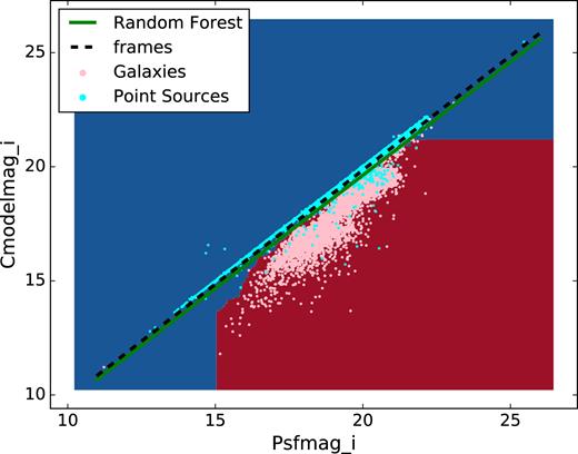
The decision boundaries generated by a Random Forest run using PSFMAG_I and CMODELMAG_I as features. The training data (pink and cyan points for spectroscopically confirmed galaxies and point sources) has been plotted over the decision boundaries (red and blue background for galaxies and point sources). The original frames method of classification is shown by the black dashed line, and the Random Forest motivated method of classification is shown by the green line.
4.4 Multiclass classification
The SDSS pipeline outputs both a classification type and subtype from the template fitting of spectra (e.g. type=point source, sub type=star or QSO). Therefore, it is possible to test machine learning algorithms with the more complex task of deciding between more classifications than just galaxy or point source.
Fig. 8 shows the decision boundaries from a Random Forest run using two photometric colours where the algorithm was asked to decide if an object was a star, galaxy, or QSO – a multiclass problem. The two colours were chosen as features for this example because they better disperse the data than using two frames features. The training process is the same as for a binary classification problem except that here the decision trees in the forest will have a fraction of leaves which identify QSOs. After a fresh hyperparameter search, we find the Random Forest achieves an object classification accuracy of 89.6 per cent. This accuracy is lower than in previous tests due to the model’s inability to accurately distinguish between stars and QSOs; this may be due to their inherent similarities as point sources. Nevertheless, this example points towards the potential of this paper’s ML methods for more extensive multiclassification problems.
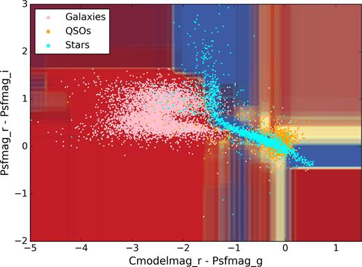
The decision boundaries generated by an example Random Forest run on a multiclass problem using two photometric colours as features. The training data (pink, cyan, and orange points for spectroscopically confirmed galaxies, point sources, and QSOs) have been plotted over the decision boundaries (red, blue, and orange background for galaxies, point sources, and QSOs).
5 CONCLUSION
Research into the area of machine learning has become prevalent in recent years, and it is important that research fields such as astronomy rapidly benefit from new modelling methods.
This paper has showcased tree-based machine learning methods by revisiting the long-standing object classification method used in the SDSS pipeline, frames, with the aim of increasing object classification accuracy using photometric data. We have developed a pipeline that offers in-depth analysis of machine learning models using treeinterpreter, which has the ability to select the most important and relevant features specific to the input data using MINT. In practice, the pipeline improves on the frames object classification accuracy by 1.0 per cent, which is ≈33 per cent improvement in the rate of misclassification (object classification error improved from ≈3 per cent to ≈2 per cent).
It can be seen from the results that while the frames method of classification performs very well, machine learning methods (especially feature driven and tuned models) can outperform them. Indeed, there are several reasons for considering methods such as those outlined in this paper.
Firstly, it has been shown that tree-based methods offer at least some level of interpretability. Machine learning models and feature selection methods such as MINT may choose to use features that do not seem to be obvious, so figuring out how and why the model is working has been difficult. With new codes such as treeinterpreter, we have shown that the models can be analysed in such a way as to provide insight into which features are important to the problem and why. Using such methods, it is possible for the machine to pick out relations/correlations that have been previously missed.
Secondly, a higher degree of classification accuracy can be achieved – one closer to that obtained by fitting spectra. The machine learning algorithms also output probabilities for each classification, allowing users to single out objects which are a problem for the machine learning model.
Thirdly, the machine learning method of classification is computationally almost as quick as the frames method. For future surveys, speed of data processing will become a very important problem. Our method could be included in the pipeline of a new survey, where a standard training set is created and given to the pipeline (from science verification data for example), and the model could be continuously improved as new data are observed.
This work is an example of how new methods like treeinterpreter and MINT are useful in understanding the relationship between data and the performance of machine learning models. This analysis would have to be repeated for new data sets from different astronomical surveys because the results presented here are not trivially transferable. In the future, as well as being incorporated into survey data processing pipelines, these methods could be applied to other problems in astronomy such as predicting redshifts or the physical properties of galaxies, and offer new insights into how and why machine learning algorithms make their decisions.
ACKNOWLEDGEMENTS
XMA would like to thank the Institute of Cosmology and Gravitation (ICG), the University of Portsmouth, and SEPNet for funding. XMA would like to thank Claire Le Cras for her helpful discussion, patience, and support. XMA would also like to thank Gary Burton for his help when using the Sciama HPC cluster.
DB is supported by Science and Technology Facilities Council (STFC) consolidated grant ST/N000668/1.
Numerical computations were done on the Sciama High Performance Compute (HPC) cluster which is supported by the ICG, SEPNet, and the University of Portsmouth.
Funding for the Sloan Digital Sky Survey III (SDSS-III) has been provided by the Alfred P. Sloan Foundation, the Participating Institutions, the National Science Foundation, and the U.S. Department of Energy Office of Science. The SDSS-III web site is http://www.sdss3.org/.
SDSS-III is managed by the Astrophysical Research Consortium for the Participating Institutions of the SDSS-III Collaboration including the University of Arizona, the Brazilian Participation Group, Brookhaven National Laboratory, Carnegie Mellon University, University of Florida, the French Participation Group, the German Participation Group, Harvard University, the Instituto de Astrofisica de Canarias, the Michigan State/Notre Dame/JINA Participation Group, Johns Hopkins University, Lawrence Berkeley National Laboratory, Max Planck Institute for Astrophysics, Max Planck Institute for Extraterrestrial Physics, New Mexico State University, New York University, Ohio State University, Pennsylvania State University, University of Portsmouth, Princeton University, the Spanish Participation Group, University of Tokyo, University of Utah, Vanderbilt University, University of Virginia, University of Washington, and Yale University.
Footnotes
Our code is hosted at https://github.com/xangma/ML_RF.
REFERENCES
,
APPENDIX A: CASJOBS SQL QUERY
This is the SQL Query submitted to CasJobs to obtain all the values required to calculate the whole sample used in this work.
select s.specObjID, s.class as spec_class, q.objid,
q.dered_u,q.dered_g,q.dered_r,q.dered_i, q.dered_z,
q.modelMagErr_u,q.modelMagErr_g, q.modelMagErr_r, q.modelMagErr_i,q.modelMagErr_z, q.extinction_u,q.extinction_g,q.extinction_r, q.extinction_i,q.extinction_z, q.cModelMag_u,q.cModelMagErr_u, q.cModelMag_g,q.cModelMagErr_g, q.cModelMag_r,q.cModelMagErr_r, q.cModelMag_i,q.cModelMagErr_i, q.cModelMag_z,q.cModelMagErr_z, q.psfMag_u,q.psfMagErr_u, q.psfMag_g,q.psfMagErr_g, q.psfMag_r,q.psfMagErr_r, q.psfMag_i,q.psfMagErr_i, q.psfMag_z,q.psfMagErr_z,
q.fiberMag_u,q.fiberMagErr_u, q.fiberMag_g,q.fiberMagErr_g, q.fiberMag_r,q.fiberMagErr_r, q.fiberMag_i,q.fiberMagErr_i, q.fiberMag_z,q.fiberMagErr_z, q.expRad_u, q.expRad_g, q.expRad_r, q.expRad_i, q.expRad_z, q.clean, s.zWarning
into mydb.specPhotoDR12 from SpecObjAll as s join photoObjAll as q on s.bestobjid=q.objid left outer join Photoz as p on s.bestobjid=p.objid
