


ABSTRACT
Fitting equilibrium dynamical models to observational data is an essential step in understanding the structure of the gaseous hot haloes that surround our own and other galaxies. However, the two main categories of models that are used in the literature are poorly suited for this task: (i) simple barotropic models are analytic and can therefore be adjusted to match the observations, but are clearly unrealistic because the rotational velocity |$v$|ϕ(R, |$z$|) does not depend on the distance |$z$| from the galactic plane, while (ii) models obtained as a result of cosmological galaxy formation simulations are more realistic, but are impractical to fit to observations due to high computational cost. Here we bridge this gap by presenting a general method to construct axisymmetric baroclinic equilibrium models of rotating galactic coronae in arbitrary external potentials. We consider in particular a family of models whose equipressure surfaces in the (R, |$z$|) plane are ellipses of varying axis ratio. These models are defined by two one-dimensional functions, the axial ratio of pressure qaxis(|$z$|) and the value of the pressure Paxis(|$z$|) along the galaxy’s symmetry axis. These models can have a rotation speed |$v$|ϕ(R, |$z$|) that realistically decreases as one moves away from the galactic plane, and can reproduce the angular momentum distribution found in cosmological simulations. The models are computationally cheap to construct and can thus be used in fitting algorithms. We provide a python code that given qaxis(|$z$|), Paxis(|$z$|), and Φ(R, |$z$|) returns ρ(R, |$z$|), T(R, |$z$|), P(R, |$z$|), |$v$|ϕ(R, |$z$|). We show a few examples of these models using the Milky Way as a case study.
1 INTRODUCTION
Since the suggestion of Spitzer (1956), the existence of hot gaseous haloes (or coronae) surrounding disc galaxies has been widely discussed (e.g. Putman, Peek & Joung 2012). In the early days their existence was uncertain and usually conjectured on the basis of early models of galaxy formation (Binney 1977; White & Rees 1978), but there is now conclusive observational evidence for the existence of such coronae.
The main and only direct observational evidence of galactic coronae comes from X-ray studies of emission and absorption lines of highly ionized species, both for the Galaxy (e.g. Yoshino et al. 2009; Gupta et al. 2012; Miller & Bregman 2013, 2015; Hodges-Kluck, Miller & Bregman 2016) and for external galaxies (e.g. O’Sullivan, Sanderson & Ponman 2007; Anderson & Bregman 2011; Bogdán et al. 2013, 2015; Walker, Bagchi & Fabian 2015; Anderson, Churazov & Bregman 2016). These observations have the potential to constrain the dynamics of the coronae in addition to their temperature and density profiles; e.g., measuring the Doppler shifts of the O vii absorption lines toward an ensemble of AGNs, Hodges-Kluck et al. (2016) ruled out a stationary halo and suggested that the hot gas contains an amount of angular momentum comparable to that in the stellar disc of the Galaxy.
For the Galaxy, indirect evidence for the presence of a corona also comes from: (i) a remarkable depletion of gas in all dwarf galaxies within |$R\simeq 270 \, {\rm kpc}$|, which is naturally explained in terms of gas ablation as the dwarfs move through a hot corona (Nichols & Bland-Hawthorn 2011; Gatto et al. 2013; Emerick et al. 2016; Tepper-García & Bland-Hawthorn 2018); (ii) observed gas stripping and tadpole morphologies in the Magellanic System, which are similarly explained as caused by hydrodynamical interaction with the coronal gas (e.g. Salem et al. 2015). Note also that the fact that the Magellanic Stream (MS) contains gas but not stars (e.g. D’Onghia & Fox 2016) and the fact that the Stream is extremely head–tail asymmetric suggest that the MS is not a purely gravitational phenomenon (e.g. Putman, Saul & Mets 2011; For et al. 2014); (iii) the measured pressures of high-velocity clouds (HVC), which are consistent with pressure equilibrium with a surrounding hot medium (Stanimirović et al. 2002; Fox et al. 2005). The disc-corona interface is also probed by the dispersion measure of pulsars with known reliable distances (Gaensler et al. 2008), which measures the integrated free electron density out to the pulsar’s distances, and by neutral-hydrogen 21cm emission data (Marasco & Fraternali 2011; Marasco, Fraternali & Binney 2012), which is present in significant amounts out to one or more kpc above the disc (note that at those heights the gas cannot be pressure supported in the vertical direction). However, due to the sparsity of observations, the properties of galactic coronae such as their mass content and extension remain largely uncertain.
Models of galactic coronae that are used in the literature for comparison with observations fall into two main categories:1 (i) simple analytic models, which are either spherical and non-rotating (e.g. Fang, Bullock & Boylan-Kolchin 2013; Tepper-García, Bland-Hawthorn & Sutherland 2015; Qu & Bregman 2018) or rotating on cylinders, so that the rotational velocity |$v$|ϕ does not depend on the distance |$z$| from the Galactic plane (e.g. Hodges-Kluck et al. 2016; Li & Bregman 2017; Pezzulli, Fraternali & Binney 2017), and (ii) those obtained as a result of cosmological simulations (e.g. Crain et al. 2010; Stinson et al. 2012; van de Voort & Schaye 2012; Ford et al. 2013; Shen et al. 2013; Bogdán et al. 2015; Velliscig et al. 2015; van de Voort et al. 2016; Correa et al. 2018; Oppenheimer 2018; Van De Voort et al. 2018). Models of type (i) have the advantage that their parameters can be adjusted to match observations, but are clearly not realistic because we know that hot haloes rotate and that their rotation velocity must decrease with height |$z$| above the galactic plane, while models of type (ii) are more realistic but cannot easily be fitted to observations, because a search in a large parameter space using simulations would be too computationally expensive. In the literature there is therefore a gap between realistic models and models that can be fitted to observations.
It is therefore important to construct more realistic analytic models which allow for an arbitrary rotation |$v$|ϕ(R, |$z$|) (which can decrease with height), and that are easy to construct and to compare with observations. In this paper, we develop a simple method that allows to construct general axisymmetric equilibria in a given external potential. The key advantage is that the method is computationally cheap and makes it easy to obtain ρ(R, |$z$|), T(R, |$z$|), P(R, |$z$|), |$v$|ϕ(R, |$z$|), and similar quantities, which can then be fed to fitting algorithms. We discuss in particular a family of models whose equipressure surfaces are ellipses, and provide an illustrative python script that constructs these models and returns the above quantities.2
The paper is structured as follows. In Section 2, we write down the basic equations. In Section 3 and 4, we describe a family of models whose equipressure surfaces are ellipses, and show some applications to the Milky Way. In Section 5, we sum up and indicate directions for future work.
2 CHARACTERIZATION OF ROTATING EQUILIBRIA
We now prove that rotating axisymmetric baroclinic3 equilibria in an external potential Φ with arbitrary entropy and angular momentum distributions are completely characterized by their pressure distribution P(R, |$z$|). In particular: (i) given P(R, |$z$|) a baroclinic equilibrium is uniquely identified and it is possible to find it constructively, and viceversa (ii) given a baroclinic equilibrium, P(R, |$z$|) is uniquely determined. Statement (ii) is trivial, so we only need to prove (i).
This provides an easy method to construct rotating baroclinic equilibria: simply choose a function P(R, |$z$|) (with the topology of surfaces of constant pressure that satisfies the constraint mentioned above), and calculate the rest. Moreover, it proves that there is a one-to-one correspondence between the ‘space of baroclinic equilibria’ and the space of the functions P(R, |$z$|) that satisfy the constraints described above.
2.1 Calculation of the other quantities
3 MODELS WITH ELLIPTICAL EQUIPRESSURE SURFACES
In Section 2, we have seen that the function P(R, |$z$|) completely characterizes baroclinic equilibria, and thus by varying this function one can in principle obtain all possible baroclinic equilibrium models. However, since |$v$|ϕ(R, |$z$|) only depends on the shape of the surfaces of constant pressure and not on the value that the pressure assumes on them, it is convenient to split the construction of an equilibrium into two steps:
Prescribe the shape of the surfaces of constant pressure.
Prescribe the value of P on the surfaces.
During the first step one can adjust the surfaces to obtain the desired |$v$|ϕ(R, |$z$|). Then the second step will determine the mass and temperature distributions of the corona.
qaxis(|$z$|): the value of the axial ratio of pressure along the axis (R = 0, |$z$|);
Paxis(|$z$|): the value of the pressure along the axis (R = 0, |$z$|).
Once these two quantities are specified, one can calculate P(R, |$z$|) and hence |$v$|ϕ(R, |$z$|), ρ(R, |$z$|), T(R, |$z$|), etc., using the equations of Section 2. In the next section, we explore some explicit models by using the Milky Way as a case study.
4 ILLUSTRATIVE APPLICATION TO THE MILKY WAY
In this section, we explore some illustrative models which are tuned to reproduce some basic properties of the Milky Way. We start with an unrealistic model 1, and step by step we adjust it to make more realistic as we go on with the numbering. Table 1 provides a summary of the models.
Models discussed in this paper. |$M_{200, \rm cor}$| and |$L_{200, \rm cor}$| are the total mass and total angular momentum of the corona contained in the virial sphere of radius |$r_{\rm 200}=237\, {\rm kpc}$|. |$L_0=10^{14}\, \mathrm{M}_\odot \, {\rm km\, s^{-1}}\, {\rm kpc}$| represents the order of magnitude of the total angular momentum contained in the Milky Way stellar disc (e.g. Peebles 1969). |$\lambda=j_{200, \rm cor} / (\sqrt{2} \, r_{200} v_{200})$| is the spin parameter according to the definition of Bullock et al. (2001), where |$j_{200, \rm cor}=L_{200,\rm cor}/ M_{200,\rm cor}$| is the averaged specific angular momentum of the corona.
| Name | qaxis | Paxis | Taxis | |$M_{200,\rm cor}/\, \mathrm{M}_\odot$| | |$L_{200,\rm cor}/L_0$| | λ |
|---|---|---|---|---|---|---|
| Model 1 | 1 (spherical) | Equation (22) | Isothermal | 3.4 × 10¹⁰ | 0 | 0 |
| Model 2 | Equations (23)–(24) | Equation (22) | Isothermal | 4.0 × 10¹⁰ | 0.91 | 0.038 |
| Model 3 | Equations (25)–(26) | Equation (22) | Isothermal | 3.9 × 10¹⁰ | 0.45 | 0.019 |
| Model 4 | 1 (spherical) | Equation (27) | Polytropic Γ = 5/3 | 2.8 × 10¹⁰ | 0 | 0 |
| Model 5 | Equations (23)–(24) | Equation (27) | Polytropic Γ = 5/3 | 3.1 × 10¹⁰ | 0.73 | 0.039 |
| Model 6 | Equations (25)–(26) | Equation (27) | Polytropic Γ = 5/3 | 3.1 × 10¹⁰ | 0.38 | 0.021 |
4.1 Potential
There is in principle no difficulty in using flattened or more complicated numerically integrated potentials to produce further models. The only constraint is to ensure that |$v_\phi ^2\gt 0$|, which requires the isobaric surfaces to be ‘flatter’ than the equipotential surfaces (see equation 7).
4.2 Normalization of the models
The data points in Fig. 1 show various estimates of density and pressure of the Milky Way corona at various distances inferred from observations (see table 7 of the review by Bland-Hawthorn & Gerhard 2016). The density estimates come from the following methods: (i) ram-pressure stripping arguments from satellite galaxies orbiting in the Galactic corona (Blitz & Robishaw 2000; Grcevich & Putman 2009; Gatto et al. 2013; Salem et al. 2015); (ii) O vi and O vii absorption (Sembach et al. 2003; Bregman & Lloyd-Davies 2007; Miller & Bregman 2013); (iii) O viii emission (Miller & Bregman 2015). The pressure estimates all essentially come from estimating the pressure of warm (|$T\gtrsim 10^4 \ \rm K$|) gas in HVCs, and then assuming that the hot corona is in pressure equilibrium with it (Stanimirović et al. 2002; Fox et al. 2005; Hsu et al. 2011).
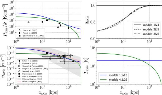
Pressure, axis ratio, density, and temperature profiles for the models discussed Section 4. The scattered points represent estimates inferred from observations.
Based on these measurements, we choose to normalize all our models so that |$n_{\rm axis}= 2 \times 10^{-4} \ \rm cm^{-3}$| at |$z=50\, {\rm kpc}$|. This approach is similar to that of Tepper-García et al. (2015) and, as also reported by them, it leads to a Galactic corona which broadly agrees with the results of observations of density over a broad range in distances. Interestingly, these models then all overestimate pressures. If instead one constructs models that match the observed pressures, density seem to be underestimated. Since measurements of pressure are all derived under the assumption of pressure equilibrium between the warm and hot medium, one possible interpretation is that the warm medium is at a slightly lower pressure than the hot medium. A similar conclusion was reached by Werk et al. (2014) that, by analysing a sample of L ∼ L* galaxies at redshift |$z$| = 0.2, found that the pressure of the warm medium was substantially lower than needed to maintain pressure equilibrium with the hot medium.
These considerations do not take into account that, since the spherical symmetry is broken in rotating coronae, one should also consider the full three-dimensional geometry (i.e. the latitude and longitude of the various data points) when comparing models to observations. Huge uncertainties remain, and the challenge will be to construct a model which is consistent with as many observational constraints as possible simultaneously.
4.3 Dispersion measures of pulsars
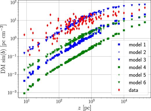
DM of pulsars with known reliable distances from observations (red diamonds) and calculated from our models. Following Gaensler et al. (2008), we show here all the pulsars that fall in one of the following three categories: (i) pulsars in the ATNF Pulsar Catalogue (Manchester et al. 2005, available at www.atnf.csiro.au/research/pulsar/psrcat) which have known parallaxes and DM; (ii) pulsars in globular clusters from the online compilation maintained by Paulo Freire at http://www.naic.edu/∼pfreire/GCpsr.html. For each globular cluster, we plot only one point corresponding to the average DM of all the pulsars (which have all similar values for the same globular cluster), and use for the distance that from globular cluster read off the catalogue of globular clusters by Harris (1996) (2010 edition), https://heasarc.gsfc.nasa.gov/W3Browse/all/globclust.html; (iii) The two pulsars in the Magellanic Clouds listed by Gaensler et al. (2008), with distances assumed to be |$50\,$| and |$61\, {\rm kpc}$| for the Large and Small Magellanic Cloud, respectively.
To calculate the DM in the models, we have assumed that the gas is completely ionized if |$T\ge 10^4\ \rm K$|, while it does not contribute if |$T\lt 10^4\ \rm K$|, and that it is composed only of hydrogen and helium with proportions |$75{{\ \rm per\ cent}}$| and |$25{{\ \rm per\ cent}}$| in mass, respectively, as suggested by big bang nucleosynthesis (e.g. Cyburt et al. 2016), so that ne = 0.75 × ρ/mp + 0.25 × 2 × ρ/(4mp) if |$T\ge 10^4\ \rm K$|. The position of the Sun is assumed to be at |$(R_\odot ,z_\odot)=(8\, {\rm kpc}, 0)$|.
4.4 Stability of the models
4.5 Models
4.5.1 Model 1
We start with the simplest possible model, which will be useful for comparison with more complicated models later: a non-rotating, isothermal model. To build this model using the framework described in the previous sections, we need to find qaxis(|$z$|) and Paxis(|$z$|).
Fig. 1 shows the density and pressure profiles obtained for model 1. They are consistent with observations within the errors, although the model seems to overestimate the pressures as discussed in Section 4.2. Fig. 2 compares the observed DM of pulsars with known reliable distances (red diamonds) and the same quantities calculated in our models. As discussed in Section 4.3, our models should provide values well below the observed ones, because the main contribution should not come from the corona but from the WIM in the disc according to Gaensler et al. (2008). Model 1 is consistent with this expectation, although not by a large margin. However, we will see in the next section that when we make this model rotating (model 2) it will fail in this regard.
The main problem of model 1 is that it is not rotating. Hence, the next step is to make it rotate.
4.5.2 Model 2
We want to modify model 1 to make it rotating. The minimal modification is to keep it isothermal along the |$z$| axis, so we can take Paxis exactly as in model 1 (this works because equation 21 is unaffected by rotation). The rotation will make it not isothermal away from the axis.
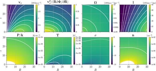
The top-right panel in Fig. 1 shows the resulting qaxis. The top panel in Fig. 3 shows the rotational velocity at different heights above the plane. The rotational velocity is higher close to the plane and decreases going up. Figs 6 and 7 show various quantities in the (R, |$z$|) plane. The contours of |$v$|ϕ in Fig. 7 roughly follow the shapes obtained in cosmological simulations (e.g. Stinson et al. 2010, 2012, 2013). The temperature decreases close to the plane, hinting at a transition with a colder disc. Linear stability analysis usually conclude that coronae are stable to the thermal instability (Binney, Nipoti & Fraternali 2009; Nipoti 2010), but assume that the gas is hot (|$T\simeq 10^6 \rm K)$|. Binney et al. (2009) find that thermal instability occurs if the coronal temperature falls through |$3 \times 10^5 \ \rm K$|, so it may be interesting to re-examine this issue using the current models, which close to the plane approach this temperature.
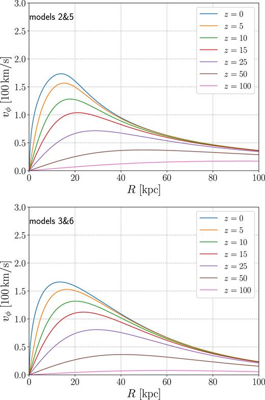
Rotational velocity at a different heights from the Galactic plane. Top panel: model 2 and 5. Bottom panel: model 3 and 6.
One problem of this model is that the DM of pulsars are too high. Making model 1 rotating has increased the DM dramatically. The reason is that the main contribution to the DM comes from regions close to the disc, and making the model rotating has made the density just above the Sun much higher (see bottom-right panel in Fig. 7 and compare with the spherical model 1). This is because now the disc is rotationally supported, and n decreases much slower as a function of R in the disc. This problem will be cured by increasing the temperature of the corona near the Galactic plane (models 4–6).
Another problem of this model is shown by Fig. 4, which shows the angular momentum distribution (AMD) for our models. The AMD is defined as the distribution of mass per unit angular momentum. Cosmological simulations typically find the AMD to be roughly exponential (e.g. van den Bosch et al. 2002; Sharma & Steinmetz 2005; Sharma, Steinmetz & Bland-Hawthorn 2012), but that of model 2 is clearly not.7 Since most of the mass is at outer radii (Fig. 5), this indicates that there is an excess of rotation (angular momentum) at large radii.
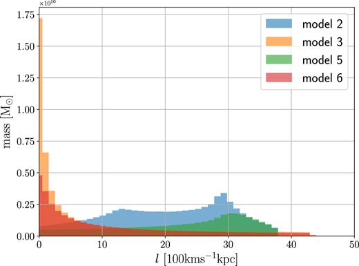
Angular momentum distribution (AMD) for our models. The AMD is defined as the amount of mass in the corona per given angular momentum.
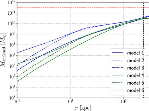
Mass enclosed within spherical radius r in our models. The black vertical dashed line indicates the virial radius r200. The red horizontal line at |$M_{200} \Omega _{\rm b}/\Omega _{\rm c}=3 \times 10^{11} \, \, \mathrm{M}_\odot$| indicates the baryons that should be contained within r200 according to the cosmological value of the ratio of baryons to dark matter, where we have taken |$\Omega _{\rm b}/\Omega _{\rm c}=18.6{{\ \rm per\ cent}}$| (Planck Collaboration VI et al. 2018).
To cure this problem, we need to modify the function qaxis. This motivates model 3.
4.5.3 Model 3
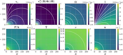
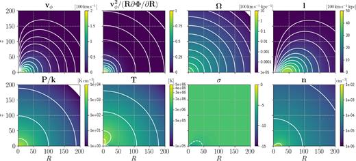
Model 2. For P/k, T, and n, the white contours coincide with labels in the colourbars. The white dashed contours for σ are at { − 5, −4, −3}.
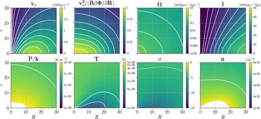
Model 2. Zoom in the innermost 30 |$\, {\rm kpc}$| of Fig. 6.
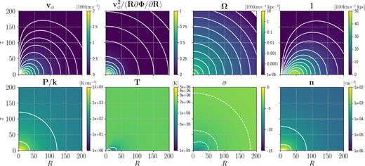
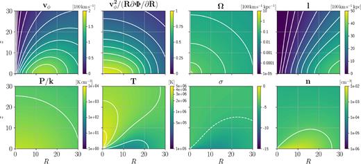
Model 3. For P/k, T, and n, the white contours coincide with labels in the colourbars. The white dashed contours for σ are at { − 5, −4, −3}.
Model 3. Zoom in the innermost 30 |$\, {\rm kpc}$| of Fig. 8.
This model retains the problem of model 2 that DM of pulsars is too high. In order to cure this problem, we need to rise the temperature of the corona close to the Galactic plane.
4.5.4 Model 4
From the bottom-left panel in Fig. 1, we see that the density profile of this model at small radii is much shallower, hence the densities are much lower at small radii. This brings down the value of the DM, which was the problem of model 3. Now we need to make this model rotating.
4.5.5 Model 5
First we try to make model 4 rotating by modifying it in the same way we modified model 1 to obtain model 2. Thus for model 5 we keep the same Paxis as model 4, but we take qaxis as in model 2. The result is shown in Figs 10 and 11. We see from Fig. 2 that this model solves the DM problem that plagued model 2 and 3, but we see from Fig. 4 that it still has the AMD problem that plagued model 2. To solve this, we can make the same modification to qaxis that we made in going from model 2 to model 3.

Model 5. For P/k, T, and n, the white contours coincide with labels in the colourbars. The white dashed contours for σ are at { − 5, −4, −3}.
Model 5. Zoom in the innermost 30 |$\, {\rm kpc}$| of Fig. 10.
4.5.6 Model 6
This model has Paxis as in model 5, thus it does not suffer from the DM problem (Fig. 2), and has qaxis as model 3, thus it does not suffer from the AMD problem (Fig. 4). The result is shown in Figs 12 and 13. This model is therefore consistent with (i) DM of pulsars with known reliable distances; (ii) the densities estimates in Fig. 1; (iii) estimates of the rotation velocity close to the plane which show it rotates roughly |$80\, {\rm km\, s^{-1}}$| slower than the disc (Marinacci et al. 2011; Hodges-Kluck et al. 2016); (iv) the roughly exponential AMD profile found in cosmological simulations (Sharma & Steinmetz 2005).
Model 6. For P/k, T, and n, the white contours coincide with labels in the colourbars. The white dashed contours for σ are at { − 5, −4, −3}.

Model 6. Zoom in the innermost 30 |$\, {\rm kpc}$| of Fig. 12.
An interesting feature of this model is that it has higher temperature lobes centred on the |$z$| axis and close to the Galactic plane, reminiscent of the Fermi bubbles (Bland-Hawthorn & Cohen 2003; Su, Slatyer & Finkbeiner 2010). By looking at X-ray absorption lines, Miller & Bregman (2013) find that while in most directions their data show little or no O viii absorption, in the direction of the Fermi bubbles (l = 338.18○, b = −26.71○) there is an enhancement of O viii. Since O viii is visible only at very high temperature (|$T \simeq 4 \times 10^{6} \ \, \rm K$|, e.g. Sutherland & Dopita 1993), this suggests that the temperature of the corona is significantly higher in the direction of the Fermi bubbles. Indeed, by analysing X-ray emission, Kataoka et al. (2013, 2015) and Miller & Bregman (2016) find that in the direction of the Fermi Bubbles the temperature rises from |$T \sim 2\times 10^6 \ $| to |$T \sim 4\times 10^6 \ \rm K$|. Our models would be consistent with these expectations, and it would be interesting to explore what dynamical effects these high-temperature lobes have once the models are allowed to evolve in time under the presence of a slow cooling and/or thermal conduction. We are not claiming that the Fermi bubbles are a consequence of our model, although we cannot exclude that the corona plays a dynamical role in producing an outflow (e.g. Waxman 1978). However, we note that a rotating halo does favour an outflow compared to a spherical halo, because it has lower density in the directions above and below the Galactic plane than within the plane (see also the models of Pezzulli et al. 2017), thus effectively clearing the way for an outflow.
This model is to a high degree isentropic (see Figs 12 and 13). This is because we have chosen Γ = 5/3. However, we have chosen this value mainly for simplicity. A model with qualitatively similar characteristics but much farther from being isentropic can be obtained taking for example Γ = 1.4. Thus, we are not ruling out models with substantial entropy gradients.
The spin parameter of all the models in Table 1 are in the range λ = 0.02–0.04. These are typical values for dark matter haloes found in simulations (e.g. Bullock et al. 2001; Sharma & Steinmetz 2005). However, by analysing a range of simulated galaxies from the eagle simulations, Oppenheimer (2018) recently found that typical spin parameters of coronae are 2–3 times higher than dark matter spin parameters (see also Danovich et al. 2015; Teklu et al. 2015). Thus it may be worth in the future to explore coronal models with higher spin parameters. This is probably best done using a flattened external potential, which would better represent a rotating dark matter halo than the spherical potential adopted in this paper.
To make progress and construct a more accurate model of the MW, we need to fit parametric models to X-ray surface brightnesses and spectra observations. This requires special care, e.g. in carefully subtracting contributions due to the Local Bubble (Sanders et al. 1977; Cox & Reynolds 1987), to the interaction between the Solar wind and interstellar neutrals (e.g. Cravens 2000; Liu et al. 2017), and to other Galactic and extragalactic sources, which is out of the scope of this paper.
5 CONCLUSIONS AND OUTLOOK
We have presented a simple method to construct general analytic equilibrium baroclinic models of galactic coronae with realistic rotations. We have considered the particular class of models whose equipressure surfaces are ellipses. These models are completely determined by the two functions Paxis and qaxis which specify the pressure and axis ratio along the axis (R = 0, |$z$|). This class of models is quite broad and can produce vastly different rotational, density, and temperature profiles. Thus it is likely that the sparse observations available can be fitted by a model of this type. Importantly, the models are computationally cheap and suited to be used in fitting algorithms and/or large parameter scans.
As an illustration of the models, we have taken the first step towards fitting dynamical models to the corona of the Galaxy. By a trial and error process, we have constructed models which are compatible with an increasing number of constraints. We have finally presented a model (number 6) which is consistent with (i) DM of pulsars with known reliable distances; (ii) the densities estimates listed in Fig. 1; (iii) the estimates of rotation velocity close to the plane being |$80\, {\rm km\, s^{-1}}$| slower than those of the disc (Marinacci et al. 2011; Hodges-Kluck et al. 2016); (iv) the roughly exponential Angular Momentum Distribution (AMD) found in cosmological simulation (e.g. Sharma & Steinmetz 2005).
The next steps are fitting increasingly complicate equilibrium models in order to exploit all the observational data available, in particular X-ray observations (Miller & Bregman 2013, 2015; Hodges-Kluck et al. 2016). This will unveil the structure of the corona in our own and other galaxies. The subsequent step will be to understand how these models evolve under the presence of a slow cooling and/or thermal conduction, and thus their connection with the problem of accretion on to the Galaxy (Pezzulli & Fraternali 2016) and of how the gas reservoir necessary to maintain star formation is replenished (e.g. Klessen & Glover 2016).
ACKNOWLEDGEMENTS
The authors thank Jeremy Bailin, Filippo Fraternali, Mordecai Mac Low, John Magorrian, Antonino Marasco, Steve Shore, Robin Tress, and Freeke van de Voort for illuminating comments and discussions. MCS and RSK acknowledge support from the Deutsche Forschungsgemeinschaft via the Collaborative Research Centre (SFB 881) ‘The Milky Way System’ (sub-projects B1, B2, and B8) and the Priority Program SPP 1573 ‘Physics of the Interstellar Medium’ (grant numbers KL 1358/18.1, KL 1358/19.2, and GL 668/2-1). ES acknowledges support from the Israeli Science Foundation under Grant No. 719/14. GP acknowledges support from the Swiss National Science Foundation grant PP00P2_163824. RSK furthermore thanks the European Research Council for funding in the ERC Advanced Grant STARLIGHT (project number 339177).
Footnotes
A notable exception are the analytic baroclinic models of Barnabè et al. (2006).
The code is publicly available at the GitHub repository coropyhttps://github.com/sormani/coropy
The word baroclinic is used here to indicate that P is a function of both T and ρ, in contrast to barotropic which indicates that P depends only on ρ.
The values displayed in the plots below are calculated assuming units of |$\, \mathrm{M}_\odot ^{1-\gamma } (100 \, {\rm km\, s^{-1}})^2 \, {\rm kpc}^{3(\gamma -1)}$|.
Note that for a spherical potential with elliptical equipressure surfaces, as we will consider in Section 4, we have |$\tan (\theta _\Phi)/\tan (\theta _P)=q^2$|. Equation (6) can be therefore rewritten as (|$v$|ϕ/|$v$|c)2 = 1 − q2, where |$v_{\rm c}^2=R \partial \Phi /\mathrm{d}R=Rg\cos (\theta _\Phi)$| is the local circular velocity of the potential. Hence in this case the surfaces of constant |$v$|ϕ/|$v$|c and the surfaces of constant q, which are the equipressure surfaces, coincide.
Indeed, Howk, Sembach & Savage (2006) compared a variety of ISM tracers, including the pulsar DM, in the foreground of the globular cluster NGC 5272 (Messier 3), which has (l, b) = (42.2○, 78.7○) and is located |$z=10\, {\rm kpc}$| above the galactic plane. They found the warm (T ∼ 104 K) and hot (T ≳ 105 K) ionized phases to be present in roughly a 5: 1 ratio along the line of sight.
Since X-ray observations mostly probe the innermost |${\lesssim }50 \, {\rm kpc}$| of the corona, we have to rely on predictions from cosmological simulations to construct the outer parts (|$R\gtrsim 50\, {\rm kpc}$|) of our models.
