


ABSTRACT
This paper reports on the validation and mass measurement of K2-263 b, a sub-Neptune orbiting a quiet G9V star. Using K2 data from campaigns C5 and C16, we find this planet to have a period of 50.818947 ± 0.000094 d and a radius of 2.41 ± 0.12 R⊕. We followed this system with HARPS-N to obtain 67 precise radial velocities (RVs). A combined fit of the transit and radial velocity data reveals that K2-263 b has a mass of 14.8 ± 3.1 M⊕. Its bulk density (|$5.7_{-1.4}^{+1.6}\, {\rm g}\,\,{\rm cm}^{-3}$|) implies that this planet has a significant envelope of water or other volatiles around a rocky core. K2-263 b likely formed in a similar way as the cores of the four giant planets in our own Solar System, but for some reason, did not accrete much gas. The planetary mass was confirmed by an independent Gaussian process-based fit to both the RVs and the spectroscopic activity indicators. K2-263 b belongs to only a handful of confirmed K2 exoplanets with periods longer than 40 d. It is among the longest periods for a small planet with a precisely determined mass using RVs.
1 INTRODUCTION
Both the Kepler mission and its revived version, the K2 mission, have discovered thousands of exoplanets, uncovering an exciting diversity in the exoplanet population (e.g. Morton et al. 2016; Mayo et al. 2018b). The modified K2 mission differs from the original Kepler mission in that it does not stare at the same field, but instead visits multiple fields in the Ecliptic Plane, each for about 80 d. This limited time span makes the mission sensitive to short-period planets only.
Only a handful of K2 exoplanets with periods longer than 40 d (half the time span of a K2 campaign) have been reported and validated.1 The planet with the longest period within the K2 campaign time span is K2-118 b. It has a period of 50.921 d and a radius of 2.49 R⊕ (Dressing et al. 2017). The faintness of the star (V ∼ 14) impedes obtaining precise radial velocities (RVs). The other validated long-period exoplanets from K2 are the three outer planets (each showing a monotransit) in the five-planet system orbiting HIP41378 (Vanderburg et al. 2016b) with estimated periods of 156, 131, and 324 d for planets d, e, and f, respectively. No mass measurements have been reported on this system yet.
Precise and accurate masses for planets similar to Earth in size with a variety of orbital periods are essential to understand the transition between rocky and non-rocky planets for small planets. Recently, a gap was found around 2 R⊕in the distribution of planetary radii of Kepler planets (e.g. Fulton et al. 2017; Zeng, Jacobsen & Sasselov 2017a; Fulton & Petigura 2018; Van Eylen et al. 2018). Planets with radii below that gap are most likely rocky or Earth-like in composition. However, without a value for the planetary mass, the composition of the planets above the gap remains uncertain.
Having a well-characterized sample of small planets spanning a broad variety of parameters, such as orbital period, planetary mass, planetary radius, and various stellar parameters (mass, radius, chemical abundances, ...), can shed light on the formation and evolution history of these planets. This can include their formation location (in terms of the snow line), the amount of planetary migration, and the effects of photoevaporation amongst other scenarios.
In this paper, we report on a four-sigma mass measurement of E K2-263b. This planet was labelled as a small planetary candidate in Mayo et al. (2018b) with an orbital period of 50.82 d and a preliminary planetary radius above the radius gap.
This paper is structured as follows. Section 2 describes the obtained data, both from photometry and spectroscopy. We validate the transit in Section 3. Stellar properties, including stellar activity indicators, are discussed in Section 4. Sections 5 and 6 describe the two analyses we performed on the light curve and RVs. Finally, we discuss and conclude in Section 7.
2 OBSERVATIONS
We recovered photometric observations from K2 and obtained spectroscopic observations from HARPS-N for K2-263 .
2.1 K2 photometry
K2-263 was observed on two occasions with NASA’s K2 mission. During Campaign 5 from 2015 April 27 till 2015 July 10, it was observed in long cadence mode (29.4 min) only.2 Campaign 16 (from 2017 December 7 till 2018 Feb 25) observed K2-263 both in long cadence and in short cadence mode (1 min).3
The data were obtained via the Mikulski Archive for Space Telescopes (MAST4) and subsequently processed following the procedures described in Vanderburg & Johnson (2014) and Vanderburg et al. (2016a). In short, we initially produced a first-pass light curve. Upon a periodicity search, a transit signal was recovered with a periodicity of 50.8 d. We then used this rough solution as a basis to extract the final light curve where we simultaneously fitted the long-term instrumental trends, the 6 h thruster systematics, and the transits.5
Due to the limited observing period of 80 d for each K2 Campaign, only two transit events occur per Campaign. The second transit in Campaign 16 could not be extracted reliably due to a brief jump in the spacecraft pointing jitter. Consequently, we have only three transit events for this target, two with long cadence and one with both long and short cadence, as seen in Fig. 2.
2.2 HARPS-N spectroscopy
We obtained 67 spectra of the G9V host with HARPS-N (Cosentino et al. 2012), installed at the Telescopio Nazionale Galileo (TNG) in La Palma, Spain. The spectra were taken between December 2015 and January 2018, each with an exposure time of 30 min. The spectra have a mean signal-to-noise ratio of 37 in order 50 (centered around 5650 Å). RVs were determined with the dedicated pipeline, the Data Reduction Software (drs; Baranne et al. 1996) where a G2 mask was used to calculate the weighted cross-correlation function (CCF; Pepe et al. 2002). The RV errors are photon-limited with an average RV error of 2.8 |$\rm m\, s^{-1}$| whilst the rms of the RVs is 3.9|$\rm m\, s^{-1}$|.
The DRS also provides some activity indicators, such as the full width at half maximum (FWHM) of the CCF, the CCF line bisector inverse slope (BIS), the CCF contrast, and the Mount Wilson S-index (SMW), and chromospheric activity indicator |$\log R^{\prime }_{\rm HK}$|from the Ca ii H&K lines (see e.g. Noyes et al. 1984; Queloz et al. 2001, 2009). Error values for the FWHM, BIS, and contrast were calculated following the recommendations of Santerne et al. (2015).
We checked each HARPS-N observation for moonlight contamination with a procedure outlined in Malavolta et al. (2017). Following this, we decided to discard the last four points, taken in January 2018 during a near-full Moon.
All RVs with their errors and activity indicators are listed in Table 1. We computed a Bayesian Generalized Lomb–Scargle periodogram (BGLS; Mortier et al. 2015) of the data, as shown in the top plot of Fig. 1. The transit period of 50.8 d is also found to be the strongest periodicity in the RV data.
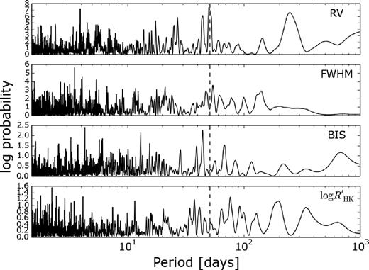
Top to bottom: BGLS periodogram of the time series of RV, FWHM, BIS, and |$\log R^{\prime }_{\rm HK}$|. The green dashed vertical line indicates the orbital period of the transiting planet.
Sample of measured RVs and activity indicators for K2-263. The full table is available online.
| Time | RV | σRV | FWHM | BIS | SMW | σS | |$\log {R^{\prime }_{HK}}$| | σRHK |
|---|---|---|---|---|---|---|---|---|
| (BJD) | (|$\rm km\, s^{-1}$|) | (|$\rm km\, s^{-1}$|) | (|$\rm km\, s^{-1}$|) | (|$\rm km\, s^{-1}$|) | (dex) | (dex) | (dex) | (dex) |
| 2457379.631593 | 29.997 16 | 0.001 76 | 6.102 95 | −0.008 40 | 0.160 672 | 0.004 935 | −5.019 180 | 0.026 653 |
| 2457380.645277 | 29.996 50 | 0.002 67 | 6.117 09 | −0.007 02 | 0.160 894 | 0.009 688 | −5.017 983 | 0.052 179 |
| 2457381.651863 | 29.999 33 | 0.002 62 | 6.092 90 | −0.005 50 | 0.157 909 | 0.009 437 | −5.034 365 | 0.052 781 |
| 2457 382.681749 | 30.001 22 | 0.004 01 | 6.051 41 | −0.001 01 | 0.165 530 | 0.016 205 | −4.993 705 | 0.082 533 |
| 2457 385.645590 | 29.993 42 | 0.003 20 | 6.092 60 | −0.001 35 | 0.150 686 | 0.012 838 | −5.076 767 | 0.079 166 |
| ... |
3 TRANSITING PLANET VALIDATION
In the recent work of Mayo et al. (2018b), K2-263 b was found to be a planet candidate with a false positive probability of 0.00292 using the probabilistic algorithm vespa (Morton 2012). They used a threshold 0.001 to validate the transit signal to be attributed to an exoplanet. Their identified planet period is 50.819 ± 0.002 d with a mid-transit time of 2457145.568 BJD. The full outcome of their analysis can be found in Mayo et al. (2018a).
The dominant false positive scenario that remained is that the star is an eclipsing binary. However, our HARPS-N observations conclusively rule that out. If the transit signal were due to an eclipsing binary, we would expect large (on the order of several |$\rm km\, s^{-1}$|) RV variations. With an RV RMS of only 3.9 |$\rm m\, s^{-1}$|, we can eliminate the scenario of an eclipsing binary. By including this eliminated scenario in the results of Mayo et al. (2018a), the false positive probability decreases to 0.000303, less than 1 in 1000, and thus statistically validating the presence of a planet orbiting K2-263.
4 STELLAR PROPERTIES
K2-263 is a G9 dwarf star, with an apparent V magnitude of 11.61. The star is located at a distance of 163 ± 1 pc as obtained via the new and precise parallax from the Gaia mission second data release (Gaia Collaboration et al. 2016, 2018). All stellar properties are listed in Table 2.
K2-263 stellar properties.
| Parameter | Value | Source |
|---|---|---|
| Designations and coordinates | ||
| EPIC ID | 211682544 | EPIC |
| K2 ID | 263 | |
| 2-MASS ID | J08384378+1540503 | |
| RA (J2000) | 08:38:43.78 | 2MASS |
| Dec. (J2000) | 15:40:50.4 | 2MASS |
| Magnitudes and parallax | ||
| B | 12.35 ± 0.03 | APASS |
| V | 11.61 ± 0.04 | APASS |
| Kepler magnitude | 11.41 | EPIC |
| J | 10.22 ± 0.02 | 2MASS |
| H | 9.81 ± 0.02 | 2MASS |
| K | 9.75 ± 0.02 | 2MASS |
| Parallax π | 6.1262 ± 0.0514 | Gaia DR2 |
| Distance d (pc) | 163.2 ± 1.4 | a |
| Atmospheric parameters: effective temperature Teff, | ||
| surface gravity log g, metallicity |$[\rm {Fe/H}]$|, projected | ||
| rotational velocity vsin i, microturbulence ξt | ||
| Teff (K) | 5372 ± 73 | b |
| log g (cgs) | 4.58 ± 0.13 | b |
| |$[\rm {Fe/H}]$| (dex) | −0.08 ± 0.05 | b |
| ξt (km s−1) | 0.76 ± 0.08 | b |
| Teff (K) | 5365 ± 50 | c |
| log g [cgs] | 4.45 ± 0.10 | c |
| |$[\rm {m/H}]$| (dex) | −0.07 ± 0.08 | c |
| vsin i (km s−1) | <2.0 | c |
| Adopted averaged parameters | ||
| Teff (K) | 5368 ± 44 | |
| log g (cgs) | 4.51 ± 0.08 | |
| |$[\rm {m/H}]$| (dex) | −0.08 ± 0.05 | |
| Mass, radius, age, luminosity | ||
| M* (M⊙) | 0.86 ± 0.03 | d |
| R* (R⊙) | 0.84 ± 0.02 | d |
| Age t (Gyr) | 7 ± 4 | d |
| L* (L⊙) | 0.55 ± 0.02 | e |
| R* (R⊙) | 0.86 ± 0.02 | e |
| M* (M⊙) | 0.87 − 0.89 | f |
| Adopted averaged parameters | ||
| M* (M⊙) | 0.88 ± 0.03 | |
| R* (R⊙) | 0.85 ± 0.02 | |
| ρ* (g cm−3) | 2.02 ± 0.16 | |
aUsing the Gaia DR2 parallax.
eUsing distance, apparent magnitude, and bolometric correction.
fRelations of Moya et al. (2018).
4.1 Atmospheric parameters
We used two different methods to determine the stellar atmospheric parameters. The first method, explained in more detail in Sousa (2014) and references therein, is based on equivalent widths. We added all HARPS-N spectra together for this method. We automatically determined the equivalent widths of a list of iron lines (Fe 1 and Fe 2) (Sousa et al. 2011) using aresv2 (Sousa et al. 2015). The atmospheric parameters were then determined via a minimization procedure, using a grid of atlas plane-parallel model atmospheres (Kurucz 1993) and the 2014 version of the moog code6 (Sneden 1973), assuming local thermodynamic equilibrium. The surface gravity was corrected based on the value for the effective temperature following the recipe explained in Mortier et al. (2014). We quadratically added systematic errors to our precision errors, intrinsic to our spectroscopic method. For the effective temperature we added a systematic error of 60 K, for the surface gravity 0.1 dex, and for metallicity 0.04 dex (Sousa et al. 2011).
Additionally, we used the stellar parameter classification tool (SPC; Buchhave et al. 2012, 2014) to obtain the atmospheric parameters. SPC was run on 63 individual spectra after which the values were averaged, weighted by their signal-to-noise ratio. The results agree remarkably well with the values from the ARES+MOOG method. As SPC is a spectrum synthesis method, it also determined a rotational velocity. This showed that K2-263 is a slowly rotating star with |$v$|sin i < 2 km s−1.
We finally adopted the average of the parameters obtained with both methods for subsequent analyses in this work. K2-263 has a temperature of 5368 ± 44 K, a metallicity of (m/H) =−0.08 ± 0.05, and a surface gravity of logg = 4.51 ± 0.08 (cgs).
4.2 Mass and radius
We obtained values for the stellar mass and radius by fitting stellar isochrones, using the adopted atmospheric parameters from the previous section, the apparent V magnitude and the new and precise Gaia parallax. We used the parsec isochrones (Bressan et al. 2012) and a Bayesian estimation method (da Silva et al. 2006) through their web interface.7 From this, we obtain a stellar mass of 0.86 ± 0.03 M⊙ and a stellar radius of 0.84 ± 0.02 R⊙. Through this isochrone fitting, we also determined a stellar age of 7 ± 4 Gyr.
The very preciseGaia parallax allows for a direct calculation of the absolute magnitude of K2-263. Extinction is negligible according to the dust maps of Green et al. (2018). Stellar luminosity can then be calculated, for which we used the bolometric correction from Flower (1996) with corrected coefficients from Torres (2010). We get a stellar luminosity of L* = 0.55 ± 0.02 L⊙. Combining with the effective temperature, this results in a stellar radius of R* = 0.86 ± 0.02 R⊙.
We furthermore employed the relations by Moya et al. (2018) to obtain a value for the stellar mass. We used three logarithmic relations between stellar mass and stellar luminosity, metallicity, and effective temperature. For these three cases, we obtained values for the stellar mass between 0.87 and 0.89 M⊙ which are in agreement with the mass value calculated above.
For the remainder of this work, we adopted the average parameters of R* = 0.85 ± 0.02 R⊙ and M* = 0.88 ± 0.03 M⊙, for the radius and mass of the star, respectively.
4.3 Stellar activity
K2-263 is a relatively quiet star as evident from the average mean value of |$\log R^{\prime }_{\rm HK}$|(−5.00 ± 0.05; see e.g. Mamajek & Hillenbrand 2008). The light curve shows no periodic variations that can be used to estimate a rotation period for this star. However, we can use the average |$\log R^{\prime }_{\rm HK}$|, together with the colour B–V to estimate the rotation period. The empirical relationships of Noyes et al. (1984; their equations 3 and 4) provide a rotation period of 35 d whilst the recipe of Mamajek & Hillenbrand (2008; their equation 5) gives 37 d. This is in agreement with the low rotational velocity determined from SPC in Section 4.1.
We investigated the periodicities in the time series of the main activity indicators (FWHM, BIS, |$\log R^{\prime }_{\rm HK}$|). Fig. 1 shows the BGLS periodograms of all three indicators. There is some variability in the indicators, but no strong periodic signals, which agrees with this star being quiet. The planet period is furthermore not present in either of the indicators, giving us confidence that the 50 d periodic signal in the RVs can indeed be attributed to the transiting planet.
Correlations between the RVs and activity indicators can be a sign of stellar variability in the RVs. We calculated the Spearman correlation coefficient for RV versus FWHM, BIS, and |$\log R^{\prime }_{\rm HK}$| and find them to be −0.09, −0.14, and 0.04, respectively, indicating no strong correlation with these indicators.
5 COMBINED TRANSIT AND RV ANALYSIS
We simultaneously modelled the K2 photometry and the HARPS-N RVs following the same procedure as described in Bonomo et al. (2014, 2015). In short, we used a differential evolution Markov chain Monte Carlo (DE-MCMC) Bayesian method (Ter Braak 2006; Eastman, Gaudi & Agol 2013). The transit model of Mandel & Agol (2002) was computed at the same short-cadence sampling (1 min) as the K2 measurements during Campaign 16. Since data of Campaign 5 were gathered only in long-cadence mode (29.4 min), we oversampled the transit model at 1 min and then averaged it to the long-cadence samples to compute the likelihood function; this allowed us to overcome the well-known smearing effect due to long integration times on the determination of transit parameters (Kipping 2010).
We accounted for a light travel time of ∼2 min between the K2 transit observations which are referred to the planet reference frame and the RVs in the stellar frame, given the relatively large semimajor axis of K2-263 b (∼0.25 AU). The free parameters of our global model are the mid-transit time Tc, the orbital period P, the systemic radial velocity γ, the RV semi-amplitude K, two combinations of eccentricity e, and argument of periastron ω (i.e. |$\sqrt{e}\cos \omega$| and |$\sqrt{e}\cos \omega$|), the RV uncorrelated jitter term sj (e.g. Gregory 2005), the transit duration T14, the scaled planetary radius Rp/R*, the orbital inclination i, and the two limb-darkening coefficients q1 and q2, which are related to the coefficients u1 and u2 of the quadratic limb-darkening law (Claret 2004; Kipping 2013). After running a first combined analysis, we noticed a curvature in the residuals of the HARPS-N RVs (see bottom plot Fig. 3). We thus decided to include an RV linear (|$\dot{\gamma }$|) and quadratic (|$\ddot{\gamma }$|) term as free parameters, following the formalism by Kipping et al. (2011). The reference time for the quadratic trend was chosen to be the average of the epochs of the RV measurements. We imposed a Gaussian prior on the stellar density as derived in Section 4.2 and used uninformative priors on all the RV model parameters. Bounds of [0, 1[ and [0, 1] were adopted for the eccentricity and the limb-darkening parameters (Kipping 2013), respectively.
We ran 28 chains, which is twice the number of free parameters of our model. The step directions and sizes for each chain were automatically determined from the other chains following Ter Braak (2006). After discarding the burn-in steps and achieving convergence according to the prescriptions given in (Eastman et al. 2013), the medians of the posterior distributions were evaluated as the final parameters, and their 34.13 per cent quantiles were adopted as the associated 1σ uncertainties. Fitted and derived parameters are listed in Table 3. The best-fitting models of the transits and RVs are displayed in Figs 2 and 3.
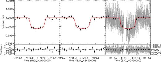
Normalized flux versus time showing the three transit events. The first two transits were observed in long cadence (29.4 min) and the third one in short cadence (1 min). The short cadence data are shown in grey with binned point overlaid in black. The red solid line indicates our best solution from the combined fit described in Section 5.
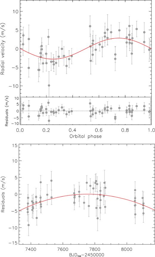
Top: RVs versus orbital phase after removing the quadratic trend. Transits occur at phase 0/1. The red line indicates the best orbital solution as a result of the combined fit. The bottom panel represents the residuals after removing both the trend and the Keplerian solution. Bottom: RVs versus time after removing the best-fitting Keplerian model for K2-263 b. The red line indicates the quadratic trend.
K2-263 system parameters from combined fit.
| Stellar parameters | |
|---|---|
| Kepler limb-darkening coefficient q1 | |$0.35_{-0.15}^{+0.19}$| |
| Kepler limb-darkening coefficient q2 | 0.51 ± 0.34 |
| Kepler limb-darkening coefficient u1 | 0.57 ± 0.39 |
| Kepler limb-darkening coefficient u2 | |$-0.01_{-0.36}^{+0.41}$| |
| Systemic velocity γ (|$\rm km\, s^{-1}$|) | 29.999 84± 0.000 59 |
| Linear term |$\dot{\gamma }(\rm m s^{-1}\, d^{-1})$|a | |$7{\rm{\small E}-04} \pm 1.9{\rm{\small E}-03}$| |
| Quadratic term |$\ddot{\gamma }(\rm m s^{-1}\, d^{-2})$|a | |$-5.40{\rm{\small E}-05} \pm 1.68{\rm{\small E}-05}$| |
| RV jitter sj | |$1.11_{-0.64}^{+0.58} (\lt\! 1.39)$| |
| Transit and orbital parameters | |
| Orbital period P (d) | 50.818 947± 0.000 094 |
| Transit epoch |$T_{ \rm c} (\rm BJD_{TDB}-2450000$|) | 8111.1274 ± 0.0012 |
| Transit duration T14 (d) | 0.1453 ± 0.0038 |
| Radius ratio Rp/R* | |$0.0260_{-0.0010}^{+0.0013}$| |
| Inclination i (deg) | |$89.24_{-0.07}^{+0.05}$| |
| a/R* | |$64.7_{-2.5}^{+2.4}$| |
| Impact parameter b | |$0.84_{-0.06}^{+0.03}$| |
| |$\sqrt{e} \cos {\omega }$| | |$0.03_{-0.23}^{+0.21}$| |
| |$\sqrt{e} \sin {\omega }$| | 0.08 ± 0.28 |
| Orbital eccentricity e | <0.14 |
| Radial-velocity semi-amplitude K (|$\rm m\, s^{-1}$|) | 2.82 ± 0.58 |
| Planetary parameters | |
| Planet mass |$M_{\rm p}\, (\rm M_\oplus )$| | 14.8 ± 3.1 |
| Planet radius |$R_{\rm p}\, (\rm R_\oplus )$| | 2.41 ± 0.12 |
| Planet density ρp (|$\rm g\,\,cm^{-3}$|) | |$5.7_{-1.4}^{+1.6}$| |
| Planet surface gravity log gp (cgs) | |$3.4_{-0.11}^{+0.10}$| |
| Orbital semimajor axis a (au) | 0.2573 ± 0.0029 |
| Equilibrium temperature Teq (K)b | 470 ± 10 |
aReference time is the average of the RV epochs.
bBlackbody equilibrium temperature assuming a null Bond albedo and uniform heat redistribution to the night-side.
By combining the derived radius ratio and the RV semi-amplitude with the stellar parameters obtained in Section 4.2, we find that K2-263 b has a radius of Rp = 2.41 ± 0.12 R⊕, a mass of Mp = 14.8 ± 3.1 M⊕, and thus a density of |$5.7_{-1.4}^{+1.6}$| g cm−3. The eccentricity is consistent with zero at the current precision.
If the RV curvature is not due to either a long-term activity variation or instrumental systematics, but instead to the presence of a long-period companion, from the |$\dot{\gamma }$| and |$\ddot{\gamma }$| coefficients we estimate the companion orbital period, RV semi-amplitude, and mass to be >4.5 yr, |$\gt 3.8\, \rm m s^{-1}$|, and >60 M⊕, respectively (e.g. Kipping et al. 2011). Without including this curvature, the semi-amplitude and thus planetary mass are slightly lower. However, the values of both analyses are within one sigma and fully consistent with each other.
6 RV ANALYSIS WITH GP
As an independent check on the mass measurement and to compare models, we performed a combined analysis of HARPS-N RVs and spectroscopic activity indices using the Gaussian process (GP) framework introduced in Rajpaul et al. (2015; hereafter R15) and Rajpaul, Aigrain & Roberts (2016). This framework was designed specifically to model RVs jointly with activity diagnostics even when simultaneous photometry is not available. It models both activity indices and activity-induced RV variations as a physically motivated manifestation of a single underlying GP and its derivative. It is able to disentangle stellar signals from planetary ones even in cases where their periods are very close (see e.g. Mortier et al. 2016), whilst at the same time not wrongly identify a planetary signal as stellar activity.
We used R15’s framework to derive a joint constraint on the activity component of the RVs and on the mass of planet b. For this analysis, we modelled the SMW, BIS, FWHM, and RV measurements simultaneously. A GP with a quasi-periodic covariance kernel was used to model stellar activity. For the GP mean function, we considered three models: zero, one, or two non-interacting Keplerian signals in the RVs only. We fixed the first Keplerian signal’s period to 50.818947 d and mid-transit time to 2458111.1274 d, as informed by the fit of the K2 light curve (see Section 5) so that this signal, if detected, would correspond to K2-263 b; we constrained the period of the second Keplerian component (to account for a possible non-transiting planet detectable in the RVs) to lie between 0.1 and 1000 d. For the prior on the orbital eccentricities we used a Beta distribution with parameters a = 0.867 and b = 3.03 (see Kipping 2013), and placed non-informative priors on the remaining orbital elements (uniform), and RV semi-amplitudes (modified Jeffreys). We also placed non-informative priors on all parameters related to the activity components of the GP framework (uniform priors for parameters with known scales and Jeffreys priors for the remaining parameters – for more details see R15). All parameter and model inference were performed using the multinest nested-sampling algorithm (Feroz & Hobson 2008; Feroz, Hobson & Bridges 2009; Feroz et al. 2013), with 2000 live points and a sampling efficiency of 0.3.
We thus computed log model likelihoods (pieces of evidence) of |$\ln \mathcal {Z}_0=-141.5\pm 0.1$|, |$\ln \mathcal {Z}_1=-135.6\pm 0.1$| and |$\ln \mathcal {Z}_2=-135.8\pm 0.1$| for the 0-, 1-, and 2-planet models, respectively. On this basis we concluded that the model corresponding to an RV detection of planet b was favoured decisively over a 0-planet model, with a Bayes factor of |$\mathcal {Z}_1/\mathcal {Z}_0\gt 300$|. The more complex 2-planet model was not supported with a Bayes factor |$\mathcal {Z}_2/\mathcal {Z}_1\sim 1.2$|.
Using the 1-planet model, we obtained an RV semi-amplitude of Kb = 2.52 ± 0.55 |$\rm m\, s^{-1}$|, and an eccentricity of |$e_b=0.08^{+0.11}_{-0.06}$| translating into a planetary mass of 13 ± 3 M⊕. This value is consistent with the one derived in Section 5. The parameters associated with this model can be found in Table 4 and the best fit is plotted in Fig. 4.
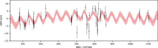
RVs versus time. The red solid line indicates the GP plus planet model posterior mean; and the shaded region denotes the ±σ posterior uncertainty. Note that the RVs were fitted jointly with activity indicator time series; however, as the GP amplitudes for the latter time series were consistent with zero, the fits for these time series are not plotted here.
| GP parameters | |
|---|---|
| GP RV semi-amplitude KGP (|$\rm m\, s^{-1}$|) | 2.68 ± 0.52 |
| GP period P (d) | |$64_{-37}^{+57}$| |
| GP inv. harmonic complexity λp | |$5.4_{-2.6}^{+2.9}$| |
| GP evolution time-scale λe (d) | |$196^{+72}_{-78}$| |
| Planet parameters | |
| System velocity γ (|$\rm km\, s^{-1}$|) | −29.837 ± 0.0015 |
| RV semi-amplitude Kb (|$\rm m\, s^{-1}$|) | |$2.52_{-0.52}^{+0.57}$| |
| Period Pb (d) | 50.818947 (fixed) |
| Eccentricity eb | |$0.08^{+0.11}_{-0.06}$| |
| Periapsis longitude ωb | |$0.97\pi ^{+0.61\pi }_{-0.58\pi }$| |
| Transit epoch Tc (BJD) | 2458111.1274 (fixed) |
| Mass Mb (M⊕) | 13 ± 3 |
| Mean density ρb (g cm−3) | 5.1 ± 1.2 |
Under the 2-planet model, the posterior distributions for Kb and eb were consistent with (and essentially identical to) those obtained under the 1-planet model. The periods of the second ‘planet’ corresponding to non-trivial RV semi-amplitudes were |$240^{+40}_{-20}$| d and 880 ± 160 d, where the first one corresponds to a peak in the RV BGLS periodogram and which may be an effect of the seasonal sampling of the data.
Under all three models, we always obtained very broad posterior distributions for the main GP hyper-parameters, indicating that the characteristics of any activity signal present were poorly constrained. In particular, under the favoured 1-planet model, we obtained |$P_\textrm{GP}=64^{+57}_{-36}$| d (overall period for the activity signal), λp ∼ 5.4 ± 2.7 (inverse harmonic complexity, with this inferred value pointing to low harmonic complexity, i.e. nearly sinusoidal variability), and |$\lambda _\textrm{e}=196^{+72}_{-78}$| d (activity signal evolution time-scale). The GP amplitude parameters for the BIS, FWHM, and SMW time series were all smaller than about |$10{{\ \rm per\ cent}}$| of the rms variation observed in each series, and indeed smaller than the estimated noise variance for each series. Thus, the GP fit suggests that there is something present in the data that is probably not simply white noise, but also cannot be interpreted as clear evidence of another planet (since the evidence for a 2-planet model is very weak) nor as activity (since no coherent signals show up in the activity indicators). Instead, these RV signals accounted for by the GP may be due to one or multiple undetected planets, instrumental or observational effects, etc.
For completeness, we have also fitted the RVs with a Keplerian without the use of a GP. Our conclusions about the planet parameters were virtually identical to and entirely consistent with those from the 1-planet plus GP model. Additionally, we ran the same analysis using a uniform prior for the eccentricity rather than the prior suggested by Kipping (2013). Again, the results were entirely consistent and thus insensitive to the choice of eccentricity prior.
7 DISCUSSION AND CONCLUSIONS
We used high-resolution spectroscopy to characterize K2-263 and determine the mass of its orbiting planet, K2-263 b. A combined analysis of the precise RVs and the K2 light curve reveals that this planet has an orbital period of 50.818947 ± 0.000094 d, a radius of 2.41 ± 0.12 R⊕, and a mass of 14.8 ± 3.1 M⊕.
Stellar contamination in the RVs can complicate the analysis and influence the planetary mass determination. Despite K2-263 being a quiet star, we ran a GP analysis of the RVs and the standard activity indicators. The mass determination agrees with the one from the combined fit. The activity indicators showed no significant variation and the GP hyperparameters were poorly constrained. As shown by the GP analysis, there are time-correlated signals in the RVs that could not be ascribed to planet b and that are not represented in the time series of the standard activity indicators. A 2-planet model, however, was not favoured for these data.
Fig. 5 shows the mass–radius diagram for all small planets (Rp < 4 R⊕) with a planetary mass determined with a precision better than 30 per cent.8 Overplotted are radius–mass relations representing different planet compositions (Zeng & Sasselov 2013; Zeng, Sasselov & Jacobsen 2016). K2-263 b has a bulk density in between that of an Earth-like rocky planet (|$32.5{{\ \rm per\ cent}}$| Fe/Ni-metal + |$67.5{{\ \rm per\ cent}}$| Mg-silicates-rock) and that of a pure-100 per cent H2O planet. Specifically, the median value of its density estimate (ρp = 5.7 ± 1.5 g cm−3) implies that it most likely contains an equivalent amount of ices compared to rocks, that is, 50 per cent ices and 50 per cent rock + metal. This proportion is expected from the abundance ratio of major planet-building elements, including Fe, Ni, Mg, Si, O, C, N, in a solar-like nebula.
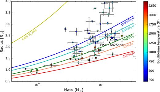
Mass–radius diagram of all planets smaller than 4 R⊕ with a mass precision better than 30 per cent (using exoplanet.eu data). The points are colour-coded according to their equilibrium temperature (assuming f = 1 and albedo A = 0). The green dots bottom left represent Venus and Earth. The solid lines show planetary interior models for different compositions, top to bottom: Cold H2/He, 100 per cent H2O, 50 per cent H2O, 100 per cent MgSiO3, 50 per cent Fe, and 100 per cent Fe. The large star represents K2-263 b, dots are planets where the mass was obtained via RV, and triangles are planets where the mass was via TTV.
Its mass of 14.8 Earth masses together with its estimated composition (half rock + metal and half ices) suggest that K2-263 b likely formed in a similar way as the cores of giant planets in our own Solar System (Jupiter, Saturn, Uranus, Neptune), but for some reason, it did not accrete much gas. This would require its initial formation beyond or near the snowline in its own system, followed by subsequent inward migration to its current position of ∼0.25 au from its host star. Considering the smaller mass (0.88 M⊙) and luminosity (0.55 L⊙) of its host star compared to the Sun, the snowline position in this particular system should be somewhat closer than it is for the Solar System. The position of the snowline in our own Solar System lies around 3 au, right in the middle of the asteroid belt (e.g. Hayashi 1981; Podolak & Zucker 2004; Martin & Livio 2012). Its location can also move inward with time (Sasselov & Lecar 2000; Sato, Okuzumi & Ida 2016). Naively scaling by the luminosity of the central star, the snowline for this system is expected to be around 2 au.
In terms of its mass and radius, K2-263 b is very similar to Kepler-131 b (Marcy et al. 2014) and HD106315 b (Barros et al. 2017; Crossfield et al. 2017), but the longer period of K2-263 b makes it significantly cooler (Teq = 470 K). In fact, K2-263 b currently has the longest period of all small planets (Rp < 4 R⊕) in Fig. 5 where the mass was determined via RVs (see Fig. 6). The only longer-period planet in this figure is Kepler-289 d (Schmitt et al. 2014) with a period of ∼66 d. However, its mass was determined via transit time variations.
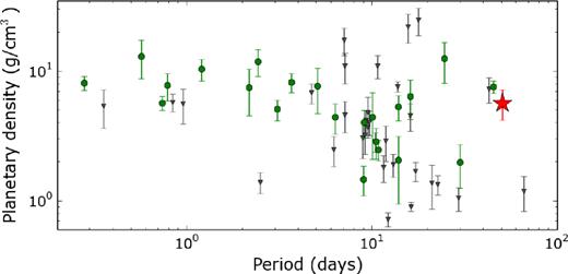
Planetary bulk density versus orbital period for the same planets as in Fig. 5. Green dots indicate the planets which mass was determined via radial velocity and grey triangles the TTV determined planets. The red star is K2-263 b.
In the mass–radius diagram, K2-263 b lies among a group of exoplanets in between 2 and 3 Earth radii with similar masses (5–20 Earth masses) and similar insolation/surface-equilibrium-temperatures. This entire group of exoplanets correspond to a peak in the planet size distribution (Zeng et al. 2018) above the recently discovered exoplanet radius gap around 2 Earth radii in the Kepler planet data (e.g. Fulton et al. 2017; Zeng et al. 2017a; Zeng et al. 2017b; Berger et al. 2018; Fulton & Petigura 2018; Thompson et al. 2018; Van Eylen et al. 2018; Mayo et al. 2018b). It means that these kind of icy cores (which must also contain rock + metal) form quite easily and favourably among solar-like stars. If correct, planets between 2 and 3 Earth radii should be in the same mass range. Simulations predict that TESS will discover 561 planets in this radius range, with about half orbiting stars brighter than V = 12 (Barclay, Pepper & Quintana 2018). Future RV observations of TESS planets could thus confirm this theory.
SUPPORTING INFORMATION
Table 1. Full table of measured radial velocities and activity indicators for K2-263.
Please note: Oxford University Press is not responsible for the content or functionality of any supporting materials supplied by the authors. Any queries (other than missing material) should be directed to the corresponding author for the article.
ACKNOWLEDGEMENTS
We thank the anonymous referee for a prompt report.
The HARPS-N project has been funded by the Prodex Program of the Swiss Space Office (SSO), the Harvard University Origins of Life Initiative (HUOLI), the Scottish Universities Physics Alliance (SUPA), the University of Geneva, the Smithsonian Astrophysical Observatory (SAO), and the Italian National Astrophysical Institute (INAF), the University of St Andrews, Queen’s University Belfast, and the University of Edinburgh.
The research leading to these results received funding from the European Union Seventh Framework Programme (FP7/2007- 2013) under grant agreement number 313014 (ETAEARTH). VMR acknowledges the Royal Astronomical Society and Emmanuel College, Cambridge, for financial support. This work was performed in part under contract with the California Institute of Technology (Caltech)/Jet Propulsion Laboratory (JPL) funded by NASA through the Sagan Fellowship Program executed by the NASA Exoplanet Science Institute (AV, RDH). LM acknowledges the support by INAF/Frontiera through the ‘Progetti Premiali’ funding scheme of the Italian Ministry of Education, University, and Research. ACC acknowledges support from the Science & Technology Facilities Council (STFC) consolidated grant number ST/R000824/1. DWL acknowledges partial support from the Kepler mission under NASA Cooperative Agreement NNX13AB58A with the Smithsonian Astrophysical Observatory. CAW acknowledges support by STFC grant ST/P000312/1. Some of this work has been carried out within the framework of the NCCR PlanetS, supported by the Swiss National Science Foundation. This publication was made possible through the support of a grant from the John Templeton Foundation. The opinions expressed are those of the authors and do not necessarily reflect the views of the John Templeton Foundation.
This material is based upon work supported by the National Aeronautics and Space Administration (NASA) under grants No. NNX15AC90G and NNX17AB59G issued through the Exoplanets Research Program. This research has made use of the SIMBAD database, operated at CDS, Strasbourg, France, NASA’s Astrophysics Data System and the NASA Exoplanet Archive, which is operated by the California Institute of Technology, under contract with NASA under the Exoplanet Exploration Program. Based on observations made with the Italian Telescopio Nazionale Galileo (TNG) operated on the island of La Palma by the Fundacion Galileo Galilei of the INAF (Istituto Nazionale di Astrofisica) at the Spanish Observatorio del Roque de los Muchachos of the Instituto de Astrofisica de Canarias. This paper includes data collected by the K2 mission. Funding for the K2 mission is provided by the NASA Science Mission directorate. Some of the data presented in this paper were obtained from the Mikulski Archive for Space Telescopes (MAST). STScI is operated by the Association of Universities for Research in Astronomy, Inc., under NASA contract NAS5-26555. Support for MAST for non-HST data is provided by the NASA Office of Space Science via grant NNX13AC07G and by other grants and contracts. K2-263 was observed as part of the following Guest Programmes: GO5007_LC (PI: Winn), GO5029_LC (PI: Charbonneau), GO5033_LC (PI: Howard), GO5104_LC (PI: Dragomir), GO5106_LC (PI: Jackson), GO5060_LC (PI: Coughlin), GO16009_LC (PI: Charbonneau), GO16011_LC (PI: Fabrycky), GO16015_LC (PI: Boyajian), GO16020_LC (PI: Adams), GO16021_LC (PI: Howard), GO16101_LC (PI: Winn), GO16009_SC (PI: Charbonneau), GO16015_SC (PI: Boyajian), and GO16101_SC (PI: Winn).
Footnotes
According to http://archive.stsci.edu/k2/published_planets/
Guest Observer programmes: GO5007_LC, GO5029_LC, GO5033_LC, GO5104_LC, GO5106_LC, and GO5060_LC.
Guest Observer programmes: GO16009_LC, GO16011_LC, GO16015_LC, GO16020_LC, GO16021_LC, GO16101_LC, GO16009_SC, GO16015_SC, and GO16101_SC
The full light curves can be obtained from https://www.cfa.harvard.edu/∼avanderb/k2c5/ep211682544.html and https://www.cfa.harvard.edu/∼avanderb/k2c16/ep211682544.html
Data from www.exoplanet.eu (Schneider et al. 2011).
