


ABSTRACT
We present a public suite of weak-lensing mock data, extending the Scinet Light Cone Simulations (SLICS) to simulate cross-correlation analyses with different cosmological probes. These mocks include Kilo Degree Survey (KiDS)-450- and LSST-like lensing data, cosmic microwave background lensing maps and simulated spectroscopic surveys that emulate the Galaxy And Mass Assembly, BOSS, and 2-degree Field Lensing galaxy surveys. With 844 independent realizations, our mocks are optimized for combined-probe covariance estimation, which we illustrate for the case of a joint measurement involving cosmic shear, galaxy–galaxy lensing, and galaxy clustering from KiDS-450 and BOSS data. With their high spatial resolution, the SLICS are also optimal for predicting the signal for novel lensing estimators, for the validation of analysis pipelines, and for testing a range of systematic effects such as the impact of neighbour-exclusion bias on the measured tomographic cosmic shear signal. For surveys like KiDS and Dark Energy Survey, where the rejection of neighbouring galaxies occurs within ∼2 arcsec, we show that the measured cosmic shear signal will be biased low, but by less than a per cent on the angular scales that are typically used in cosmic shear analyses. The amplitude of the neighbour-exclusion bias doubles in deeper, LSST-like data. The simulation products described in this paper are made available at http://slics.roe.ac.uk/.
1 INTRODUCTION
The standard model of cosmology has been highly successful in describing a number of observations, including fluctuations in the cosmic microwave background (CMB, e.g. Das et al. 2014; Planck Collaboration 2016), and baryonic acoustic oscillations in galaxy surveys (e.g. Blake et al. 2011; Padmanabhan et al. 2012; Alam et al. 2017a). The technique of weak gravitational lensing has recently seen rapid progress, resulting in the early results from the Kilo Degree Survey (KiDS) and the Dark Energy Survey (DES) presented in Hildebrandt et al. (2017, H17 hereafter) and Troxel et al. (2017), respectively. Based on the measurement of correlations between the shapes of distant galaxies that are produced by a foreground matter distribution, the weak-lensing signal is a key probe of dark matter and structure formation (see Bartelmann & Schneider 2001, for a review).
To reach its full potential, this technique must address a number of systematic effects (Massey et al. 2013; Mandelbaum 2017), many of which are associated with the fact that the scales probed by the signal reside in the non-linear regime of gravitational collapse. Complications therefore arise due to non-linear dynamics, which generate important deviations from linear predictions and produce non-Gaussian features in the matter distribution that can affect likelihood analyses. Many of these challenges can be overcome with numerical N-body simulations, which accurately capture the gravitational physics over the scales relevant to the weak-lensing measurement. These calculations are expensive to carry out and require vast resources on supercomputers, but their scientific outcome is rich and their applications numerous and central to many aspects of weak-lensing analysis:
Modelling – Numerical cosmological simulations are required in the modelling of weak-lensing signals for which theoretical predictions are either not available or not accurate enough. Modern prediction tools such as halofit (Smith et al. 2003; Takahashi et al. 2012), the Cosmic Emulator (Heitmann et al. 2014), hmcode (Mead et al. 2015) or the Mira-Titan project (Heitmann et al. 2016) are all based on large suites of N-body simulations in which the input cosmology parameters were varied. The science objectives were, in these cases, to construct high-precision predictions of the two-point correlation functions (for the collisionless dark matter) that extend deep into the non-linear regime of large-scale-structure formation. In the context of weak lensing, these serve to model the cosmic shear signal. On top of this, there are complementary lensing measurements that are particularly sensitive to non-linear structures and which contain additional information, such as the lensing peak statistics (e.g. Liu et al. 2015a,b; Kacprzak et al. 2016; Martinet et al. 2017), the lensing of under- and overdense regions (Friedrich et al. 2017; Gruen et al. 2017; Brouwer et al. 2018), or clipped lensing (Simpson et al. 2016; Giblin et al. 2018), which in some cases completely rely on simulations to estimate the expected signal. It is worth mentioning here that an important part of the modelling comes from the presence (or the absence) of massive neutrinos, modified gravity and baryon feedback. However, these effects are outside the scope of this paper, and can be dealt with separately with analytic halo models (e.g. Mead et al. 2016) or hydrodynamical simulations (e.g. Semboloni et al. 2011; McCarthy et al. 2018; Chisari et al. 2018).
Validation of estimators – In addition to their key role in the modelling of weak-lensing observables, simulations can be post-processed into mock catalogues that are constructed to match a number of properties of the input data. In that form, the mocks serve to test, calibrate and optimize different estimation techniques, and can tell us how these respond to different observational effects that can be added by hand (e.g. survey masking, photometric error, and point spread function residuals). Another usage is to test the sensitivity of different measurement techniques to known systematic contamination. This is of particular importance when developing new weak-lensing estimators, e.g. clipped lensing, and study their response to secondary physical effects such as source clustering.
Covariance matrix estimation – Weak-lensing analyses are carried out on correlated data points, which means that an accurate assessment of the uncertainty on the measurements requires a full covariance matrix. The ideal way to measure this relies on a large ensemble (LE) of independent N-body simulations at each of the cosmologies that are being sampled along the Monte Carlo Markov Chain (MCMC) parameter sampler. Given the requirement that the number of simulations per ensemble must significantly exceed the dimension of the data vector, this scenario requires computing resources far exceeding those currently available. Alternative techniques have been used instead to estimate the covariance matrices of weak-lensing observables, including ‘internal’ estimates such as jack-knife (JK) or bootstrap resampling of the data, analytic calculations (see Takada & Jain 2009; Krause & Eifler 2017, for example), lognormal realizations (Hilbert, Hartlap & Schneider 2011), or approximate gravity solvers such as ICE-COLA (Izard, Fosalba & Crocce 2018). Another approach is to run an ensemble of full N-body simulations at a single cosmology and ignore the variation of the covariance with cosmology. Hybrid techniques are also possible, where for example one can use fast Gaussian approximations to promote a matrix with some cosmological dependence (see Kilbinger et al. 2013, for example). Each of these techniques have pros and cons, and the best choice for a given measurement will strike a compromise that minimizes the impact on the final parameter inference. Generally, internal estimates become inaccurate at large scales, lognormal, and approximate methods do not reproduce exactly the non-linear structures, analytical calculations need to be validated against ensembles of N-body simulations to begin with, and simulation-based estimates are themselves subjected to the missing ‘Super Sample Covariance’ (SSC) term (Li, Hu & Takada 2014). Undoubtedly, even at a fixed cosmology, the ensemble approach offers a valuable tool to estimate covariance matrices, which is the central focus of this paper.
Likelihood modelling – Weak-lensing analyses are mostly carried out under the assumption that the underlying data are distributed according to a multivariate Gaussian function. The likelihood that describes such idealized data can be expressed analytically, however little is known about the accuracy of this assumption. In fact, this is expected to break in the highly non-linear regime, and there are even hints that this could already be a source of systematic error in the interpretation of the current weak-lensing data (Sellentin & Heavens 2016). There is a need to study extensions to the current method, and numerical simulations can serve to test non-Gaussian likelihood models (Sellentin, Heymans & Harnois-Déraps 2018; Hahn et al. 2018). These assumptions and their numerical implementation can be tested in a full mock analysis, where it can be verified whether the likelihood analysis can recover the input cosmology (MacCrann et al. 2018).
There is a range of public mock data sets designed to serve the weak-lensing community, each having their strengths and limitations.1 We present a few of them here, and summarize in Table 1 some of the key properties that affect their performance at estimating weak-lensing covariance matrices. Ray tracing through the Millennium Simulation (Springel et al. 2005; Hilbert et al. 2009), for instance, has yielded a rich science outcome, however there is only one realization (and two cosmologies). The MICE-GC simulation (Fosalba et al. 2013) is particularly useful for the volume it covers, but again there is a single realization available . Complementary to these are the Dietrich & Hartlap (2010, DH10 hereafter) simulations, which probe 158 different cosmologies in the [σ8 − Ωm] plane, and additionally contain an ensemble of 37 realizations for the main cosmology. Compared to the other simulations, this large suite was constructed with smaller volumes and at a lower mass resolution.
Properties of some of the weak-lensing simulations that are publicly available: Lbox is the comoving side length of the simulation box, mp is the particle mass, Ncosmo is the number of cosmologies available, Nsim is the number of realizations, and Atot is the total area, combining all cosmologies and realizations. The second cosmology covered by the Millennium Simulation is obtained by post-processing the first one (Angulo & White 2010) hence is not independent. The particle mass varied with cosmology in the DH10 simulations, while both mp and Lbox varied with redshift in the HSC simulations, in 11 steps between |$z$| = 0 and 3. The 108 realizations of the HSC mocks are not fully independent: 18 light-cones are produced from each of the 6 truly independent volumes. Nsim = 932 for the SLICS comic-shear and CMB lensing data, and 844 for the full set of probes.
| SLICS | HSC | DH10 | CLONE | MICE-GC | Millennium | |
|---|---|---|---|---|---|---|
| Lbox (h−1Mpc) | 505 | 450 (|$z$| ∼ 0) | 140 | 231.1 (|$z$| > 2) | 3072 | 500 |
| 4950 (|$z$| ∼ 3) | 147.0 (|$z$| < 2) | |||||
| mp (h−1M⊙) | 2.88 × 10⁹ | 8.2 × 10⁸ (|$z$| ∼ 0) | 6.51 × 10⁹(Ωm = 0.07) | 8.94 × 10⁸ (|$z$| > 2) | 2.93 × 10¹⁰ | 8.6 × 10⁸ |
| 1.1 × 10¹² (|$z$| ∼ 3) | 5.74 × 10¹⁰(Ωm = 0.62) | 2.30 × 10⁸ (|$z$| < 2) | ||||
| Ncosmo | 3 | 1 | 158 | 1 | 1 | 2 |
| Nsim | 844 | 108 | 192 | 185 | 1 | 1 |
| Atot (deg2) | 8.44 × 10⁴ | 4.45 × 10⁶ | 6912 | 2.37 × 10³ | 1.03 × 10⁴ | 1024 |
The CLONE catalogue (Harnois-Déraps, Vafaei & Van Waerbeke 2012) was specifically tailored for data quality assessment and covariance estimation in weak-lensing data analyses of the Canada–France–Hawaii Telescope Lensing Survey (Heymans et al. 2012). With 185 realizations, the CLONE probes very small scales, but also suffers from small volumes (the box sizes are 231 and 147 h−1 Mpc on the side, depending on the redshift) at a level that is now inadequate for the current generation of lensing surveys.
An ensemble of 108 full-sky weak-lensing mock data has also been produced by Takahashi et al. (2017) and made publicly available, combined with a release of dark matter halo catalogues and CMB lensing maps. These simulation products are designed for the Hyper Suprime Camera (HSC) weak-lensing survey, but can serve broader science cases. Being full sky, these ‘HSC’ mocks are well suited to test estimators acting on spherical coordinates, such as curved-sky map reconstruction algorithms. While there are 108 realizations in the release, these mocks are not statistically independent, having ‘recycled’ a smaller number of truly independent N-body realizations. It has been shown that such recycling has little impact on the cosmic shear covariance matrix (Petri, Haiman & May 2016), however its effect on higher order statistics and likelihood modelling is still unknown. The finite mass resolution of these simulations can be limiting for some applications, since the minimal halo mass that they form gradually varies from |$1\times 10^{12}\ h^{-1}\, \mathrm{M}_{\odot }$| at |$z$| ∼ 0.3–|$5\times 10^{13}\ h^{-1}\, \mathrm{M}_{\odot }$| haloes at |$z$| ∼ 3 (see their fig. 3). This is insufficient to describe many galaxy populations that reside in less massive systems, but can serve to model low-redshift luminous red galaxies (LRGs), which are hosted in |$1\times 10^{12}\ h^{-1}\, \mathrm{M}_{\odot }$| haloes (see Section 3.3 and Fig. 7). According to these limitations, a |$z$| ∼ 0.7 LRG sample based on these HSC mocks would be missing its least massive members. However, their large volumes make these HSC mocks particularly suitable for the evaluation of the SSC term.
The SLICS (Scinet LIght Cone Simulations, described in Harnois-Déraps & van Waerbeke 2015, HvW15 hereafter) were designed as a massive upgrade of the CLONE. With a volume of Lbox = 505 h−1Mpc on the side, they significantly reduce the limitations caused by the finite-box size, thereby allowing data analyses that include larger angular scales (the cosmic shear signal is valid out to 2 deg, as opposed to about half a degree in the CLONE). They resolve structure deep within the non-linear regime, and the larger size of the ensemble supports longer data vectors without introducing high levels of noise in the covariance matrix. The SLICS were first tailored for the Red-Sequence Clusters Lensing Survey (Hildebrandt et al. 2016), and later reprocessed for the cosmic shear analysis presented in H17, which is based on the first 450 deg2 of the KiDS data. This flexibility is one of the highlights of numerical simulations: once the lensing data have been computed and stored on disk, it is relatively inexpensive to reproduce the properties of many different surveys.
This paper presents a significant expansion of the SLICS suite from its original version, with a focus on cross-correlation science. On top of the weak-lensing mass and shear planes introduced in HvW15, we present here the KiDS-450- and the LSST-like ‘source’ catalogues, which emulate the two photometric surveys they are named after. We also describe the backbone dark matter halo catalogues as well as three mock ‘lens’ galaxy catalogues that reproduce properties of the CMASS and LOWZ LRG samples (Reid et al. 2016) that are part of the Baryon Oscillation Spectroscopic Survey (BOSS), and the denser galaxy sample from the Galaxy And Mass Assembly spectroscopic survey (Liske et al. 2015, GAMA hereafter) . We construct an additional set of galaxy catalogues (KiDS-HOD and LSST-like HOD) specially designed to study systematic and selection effects related to source–lens coupling (Hartlap et al. 2011; Yu et al. 2015), and finally supplement the light-cones with simulated lensing maps of the CMB. As a direct application, we construct a combined-probe data vector that incorporates cosmic shear, galaxy–galaxy lensing, and galaxy clustering and present the full covariance matrix.
Many of these simulation products already served in cosmological analyses: the cross-correlation of weak lensing with Planck lensing (Harnois-Déraps et al. 2016, 2017), cosmic shear (H17), peak statistics (Martinet et al. 2017), combined-probe analyses with redshift-space distortions (RSD, Joudaki et al. 2017; Amon et al. 2018a) and galaxy clustering (van Uitert et al. 2018), clipped lensing (Giblin et al. 2018), and density-split statistics (Brouwer et al. 2018). The first part of this paper therefore serves as a reference for those interested in the different SLICS products, where we detail their design, performance, and limitations.
In the second part of this paper, we revisit the neighbour-exclusion bias, a subtle selection effect first reported in Hartlap et al. (2011) and revisited by MacCrann et al. (2017), sourced from the fact that objects with close neighbours are more common in regions with foreground clusters than with foreground voids. Positions and shapes are more difficult to extract for these objects, hence they are typically rejected or downweighted in weak-lensing analyses. This selection therefore preferentially downsamples regions with the highest density of foreground galaxies, which also correspond to regions that yield the highest lensing signal. This is a form of source–lens coupling unrelated to the photometric uncertainty or contamination by cluster members, and which affects the cosmic shear signal over a wide range of scales. We first investigate this neighbour-exclusion bias in the context of a weak-lensing survey at KiDS depth, including tomographic decomposition, different levels of close-pairs exclusion, and two different strategies to deal with them, then extend this measurement to LSST depth.
This paper is structured as follow. We review the configuration of the N-body runs, our strategy to extract lensing maps and dark matter haloes in Section 2. We then describe our different galaxy catalogues in Section 3, we list the caveats and limits that are known to affect the numerical products, and conclude the first part of this paper by presenting the combined-probe covariance matrix in Section 4. We next investigate the neighbour-exclusion bias in Section 5, and conclude in Section 6. We finally present complementary information about some of the mock products in the appendices.
2 DARK MATTER LIGHT-CONES
2.1 The N-body calculations
The SLICS are based on a series of 1025 N-body simulations produced by the high performance gravity solver CUBEP3M (Harnois-Déraps et al. 2013). They were first presented in HvW15, and we report here some of the key properties. The fiducial cosmology adopts the best-fitting WMAP9 + BAO + SN parameters (Hinshaw et al. 2013), namely: Ωm = 0.2905, |$\Omega _\Lambda = 0.7095$|, Ωb = 0.0473, h = 0.6898, σ8 = 0.826, and ns = 0.969. This choice lies close to the mid-point between the cosmic shear and the Planck best-fitting values in the [σ8 − Ωm] plane. Each run follows 15363 particles inside a grid cube of comoving side length |$L_{\rm box} = 505 \ h^{-1}\, {Mpc}$| and nc = 3072 grid cells on the side, starting from a set of initial conditions at |$z$|i = 120 obtained via the Zel’dovich approximation. The N-body code computes the non-linear evolution of these collisionless particles down to |$z$| = 0 and generates on-the-fly the halo catalogues and mass sheets required for a full light-cone construction (see Sections 2.2 and 2.3). By construction, this setup makes no distinction between baryons and dark matter, and ignores the impact of massive neutrinos.
The complete SLICS series consists of a core ‘Large Ensemble’ (the SLICS-LE suite) of 932 fully independent realizations, augmented with five runs in which the gravitational force is resolved to smaller scales (with the extended particle–particle mode described in Harnois-Déraps et al. 2013). These extra runs make up the SLICS-HR suite, which served for convergence tests of the SLICS-LE. We also produced an additional 73 runs at σ8 = 0.861, and 15 with σ8 = 0.817 and ns = 0.960. Although restricted in their sampling of the parameter space, these runs enable some sensitivity tests to differences in cosmology. This paper solely focuses on the development of simulation products performed in the LE, which we hereafter refer to as the ‘SLICS simulations’.
Each of the SLICS realizations required 64 mpi processes, running on either 8 or 16 cpus in an openmp parallelization mode, for a total of 512–1024 cores depending on the machines. The real runtime to reach |$z$| = 0 on the Compute Canada SciNet-GPC and Westgrid-Orcinus clusters (intel x86 processors) was about 30 h per simulation, depending on the architecture, on the network usage, and on the level of non-linear structures formed inside the cosmological volume. CUBEP3M does not explicitly enforce load balance across the compute nodes, hence a super-structure forming inside one node will require more time to resolve, effectively slowing down all nodes. With six phase-space elements per particle at 4 bytes each, a single particle dump takes up 87 GB of disk space. Given our need for multiple redshift checkpoints for over 1000 realizations, storing the particle data was not an option. Once halo catalogues and mass sheets were generated, the particles were deleted (with the exception of the SLICS-HR suite, for which the particle data will be made available upon request).
The particle mass is set to |$2.88\times 10^{9} \ h^{-1}\, \mathrm{M}_{\odot }$|, thereby resolving dark matter haloes below |$10^{11} \ h^{-1}\, \mathrm{M}_{\odot }$| and structure formation deep in the non-linear regime. The 3D dark matter power spectrum, P(k), agrees within 2 per cent with the SLICS-HR as well as with the predictions from the Extended Cosmic Emulator (Heitmann et al. 2014) for Fourier modes |$k\lt 2.0 \ h\, {\rm Mpc}^{-1}$| (fig. 6 of HvW15). Higher k modes (corresponding to smaller scales) are affected by finite force/mass resolution, such that at k = 5.0 |$(10.0) \ h\, {\rm Mpc}^{-1}$|, the simulated P(k) from the SLICS is 15 per cent (50 per cent) lower than the emulator, which achieves 5 per cent precision up to k = 10 h Mpc−1. This resolution limit inevitably propagates into the light-cone, which then also impacts the projected measurements such as the shear two-point correlation function or the convergence power spectrum (see figs 1 and 7 in HvW15). As always, mass resolution needs to be considered when deciding on the scales at which the cosmic shear results from SLICS are reliable; this is further discussed in HvW15 and in Section 3.1.
2.2 Gravitational lenses
We construct flat-sky weak-lensing maps with the multiple-plane tiling technique (in many aspects similar to Vale & White 2003), in which convergence and shear maps are extracted from a series of 18 mass sheets under the Born approximation. When the simulation reaches pre-selected lens redshifts, |$z$|l, the particles from half the cosmological volume are projected along the shorter dimension on 2D grids of |$12\, 288^2$| pixels following a ‘cloud in cell’ interpolation scheme (Hockney & Eastwood 1981). This process is repeated for the three Cartesian axes, however we keep on disk only one of these mass planes per redshift following a regular sequence (e.g. xy, xz, yz, xy, ...). The redshifts of these planes, reported as |$z$|l in Table 2, are chosen such that the half volumes continuously fill the space from |$z$| = 0 to 3. This requires 18 planes in the adopted cosmology. Starting from the observer at |$z$| = 0, the first mass plane corresponds to the projection of the comoving volume in the range [0 – |$252.5\ h^{-1}\, {Mpc}$|], which we assign to its centre (at |$126.25 \ h^{-1}\, {Mpc}$|, or |$z$|l = 0.042); the second plane projects the volume [252.5–|$505\ h^{-1}\, {Mpc}$|], also assigned to its centre (at |$378.75\ h^{-1}\, {Mpc}$|, or |$z$|l = 0.130), and so on for all 18 planes. We turn these density maps into overdensity maps by subtracting off the mean.
Lens and source redshift planes used to construct our past light-cones. These are obtained by stacking half boxes, each |$252.5 \ h^{-1 }\, {Mpc}$| thick, from the observer out to |$z$|max ∼ 3.0. The lens planes lie at the centre of the projected volumes, and the ‘natural’ source planes correspond to the back of each half box.
| |$z$|l | 0.042 | 0.130 | 0.221 | 0.317 | 0.418 | 0.525 | 0.640 | 0.764 | 0.897 | 1.041 | 1.199 | 1.373 | 1.562 | 1.772 | 2.007 | 2.269 | 2.565 | 2.899 |
|---|---|---|---|---|---|---|---|---|---|---|---|---|---|---|---|---|---|---|
| |$z$|s | 0.086 | 0.175 | 0.268 | 0.366 | 0.471 | 0.582 | 0.701 | 0.829 | 0.968 | 1.118 | 1.283 | 1.464 | 1.664 | 1.886 | 2.134 | 2.412 | 2.727 | 3.084 |
We carve out our light-cones2 by shooting rays on a regular grid of 77452 pixels with an opening angle of 100 deg2, which corresponds to the angular extension of the simulation box at redshift |$z$| = 1.36. We extend the light-cones up to |$z$| = 3 by using periodic boundary conditions to fill in regions of the mass sheets that fall outside the volume. The light-cone overdensity mass maps, which we label |$\delta _{\rm 2D}({\boldsymbol \theta }, z_{\rm l})$|, are obtained from a linear interpolation of the mass overdensity sheets onto the mock pixels |${\boldsymbol \theta }$| after randomly shifting the origins . This translation, together with the sequential change of the projection axis mentioned above, are designed to minimize the repetition of structure across redshift when constructing a light-cone from a single N-body run.
Samples of these mass overdensity maps are presented in Fig. 1. One direct consequence of this procedure is that correlations in the matter field are explicitly broken between boxes. This is important to note when measuring 3D quantities within the SLICS light-cones.

Sample of the different simulation products presented in this paper. The background colour maps represent 256 h−1 Mpc of projected dark matter, the red circles show the dark matter haloes with sizes scaling with their mass, and the large and small yellow squares show the central and satellite galaxies, respectively. The left-hand panels shows the GAMA galaxies centred at redshift |$z$| = 0.221, the central panel shows the LOWZ galaxies centred at |$z$| = 0.317, while the right-hand panel shows the CMASS galaxies, centred at |$z$| = 0.640. These three mock galaxy samples are described in Sections 3.3–3.5. The side length of the three panels each subtend half a degree.
2.2.1 CMB lensing maps
For each of the light-cones, we also produced convergence maps that extend to |$z$|s = 1100, which were described and used in Harnois-Déraps et al. (2016) for the validation of combined-probe measurement techniques involving CMB lensing data. These κCMB maps were constructed in a hybrid scheme: a single set of 10 mass planes were generated from linear theory to fill the volume between 3.0 < |$z$| < 1100. They were first smoothed to reduce shot noise, then placed at the back end of each of the main SLICS light-cones, enabling ray tracing up to the CMB for all lines of sight.
The fact that the same back-end volume is used for each of the κCMB maps effectively couples the maps across different lines of sight, which means that the covariance matrix of the autospectrum (or autocorrelation function) of these κCMB maps will be wrong. However, these maps are primarily constructed for the study of combined probes, hence any cross-correlation measurement with |$z$| < 3.0 mock data will only see the main SLICS light-cone hence the covariance will not be affected by this.
We additionally produced a series of κCMB maps that reproduce the Planck lensing measurements, which we obtained by adding noise maps with the noise spectrum given by in the data release3, followed by a Fourier filtering procedure that removes the ℓ > 2048 modes, as in the data (Planck Collaboration et al. 2016). These maps are constructed with the same foreground matter fields hence can serve for estimator validation and covariance estimation in cross-correlation analyses involving the Planck lensing data.
2.2.2 Data products: lensing maps
For all 932 light-cones, we provide the following lensing maps:
|$\delta _{\rm 2D}(\chi _{\rm l},{\boldsymbol \theta })$| for the 18 lens planes (|$z$|l) listed in Table 2
|$\gamma _{1,2}(\boldsymbol \theta)$| for the 18 source planes (|$z$|s) listed in Table 2
Noise-free |$\kappa _{\rm CMB}(\boldsymbol \theta)$| convergence maps
Planck-like |$\kappa _{\rm CMB}(\boldsymbol \theta)$| convergence maps
These are all flat-sky, 100 deg2 maps with 77452 pixels, stored in fits format. The mass maps can be used to recreate convergence and shear maps with any redshift distribution if needed, while the shear maps can be populated with a galaxy catalogue of arbitrary n(|$z$|) in the range [0.0, 3.0] and used to assign shear to each object.
2.3 Dark matter halo catalogues
Dark matter haloes serve as the skeleton for the galaxy population algorithms used in this paper (Sections 3.2–3.6), hence we document their key properties in this section. We identify haloes using a spherical overdensity algorithm (detailed in Harnois-Déraps et al. 2013), which first assigns particles onto the fine simulation grid, then looks for maxima and ranks them in descending order according to their peak height. The halo finder then grows a series of spherical shells over each maximum until the total overdensity (with respect to the cosmological background) falls under the threshold of 178.0, in accordance with the top-hat spherical collapse model. Particles within the collapse radius are then re-examined in order to extract a number of halo properties, including the halo mass, the position of its centre of mass and of its peak, the velocity dispersion for all three dimensions, its angular momentum and inertia matrix. We reject haloes with less than 20 particles, which introduces a low-mass cut-off in the reconstructed halo catalogue at |$M_{\rm h,min} = 5.76\times 10^{10} \ h^{-1}\, \mathrm{M}_{\odot }$|. In this process, particles cannot contribute to more than one halo.
The mass function of these haloes reproduces the results expected from predictions by Sheth et al. (2001), as shown in Fig. 2. We also show in Fig. 3 the halo bias bh at |$z$| = 0.042 for four mass bins. This quantity was extracted from the simulation by computing the power spectrum of the halo catalogues, |$P_{\rm halo}(M_{\rm h},k,z) = \langle |\delta _{{\rm halo}, M_{\rm h}}(k,z)|^2\rangle$|, and that of the particle data, P(k, |$z$|) = 〈|δ(k, |$z$|)|2〉. The halo density |$\delta _{{\rm halo}, M_{\rm h}}(x,z)$| is constructed by placing haloes in mass bin Mh and redshift |$z$| on a 30723 grid, which is Fourier transformed, squared, and angle-averaged to obtain the halo power spectrum. We repeat this procedure with the full particle data to obtain δ(k, |$z$|) and P(k, |$z$|), and extract the bias via the relation |$b^2_{\rm h}(M_{\rm h},z,k) = P_{\rm halo}(k,z,M_{\rm h})/P(k,z)$|. Note that this numerical computation provides only the two-halo term contribution to the power spectrum, which is enough to estimate the linear bias. The one-halo term would require sub-halo catalogues, which we have not constructed. In this calculation, the particle and halo mass assignment scheme was corrected for by dividing the power spectra by the window function (Hockney & Eastwood 1981), but the shot noise was not subtracted.

The halo mass function at |$z$| = 0.22 in the full simulation box and in the light-cone, compared to predictions from Sheth, Mo & Tormen (2001). Error bars show the error on the mean, obtained from 100 lines of sight. The agreement is similar at other redshifts.

Halo bias in the mocks for redshift |$z$| = 0.042 in four wide mass bins, labelled in the figure in units of |$\, \mathrm{M}_{\odot }$|. Poisson shot noise is not subtracted, and the error is on the mean, estimated from 100 realizations. Shown with the red dashed lines are the linear bias predictions from Tinker et al. (2010).
Looking at the linear regime (k < 0.05 h Mpc−1), we clearly see that the most massive haloes are the highest biased tracers of the underlying dark matter field, and that haloes in the mass range |$[10^{11}\text{--}10^{13}] \ h^{-1}\, \mathrm{M}_{\odot }$| have a bias lower than 1.0. Our measurements are in excellent agreement with the predictions from the spherical collapse model of Tinker et al. (2010) for the largest three mass bins plotted in Fig. 3, however the |$[10^{11}\text{--}10^{12}] \ \, \mathrm{M}_{\odot }$| haloes exhibit a bias that is 14 per cent higher than the predictions, (bh = 0.82 in the mocks, compared to the predicted value of 0.72). The size of this deviation is similar to the differences between linear bias models (e.g. Mo & White 1996; Sheth et al. 2001; Sheth & Tormen 1999) which means that our halo clustering agrees well with the models within the theoretical accuracy. The linear bias approximation holds well at large scales (|$k\lt 0.1 \ h\, {\rm Mpc}^{-1}$| for haloes with |$M_{\rm h}\lt 10^{14} \, \mathrm{M}_{\odot }$|, smaller k modes for heavier haloes). The bias bh(k) in all mass bins deviates from the horizontal at |$k\gt 0.2 \ h\, {\rm Mpc}^{-1}$|, in part because of the shot noise, in part because of the non-linear bias (which we do not attempt to model in this paper). We note, however, that the shape of the non-linear bias heavily depends on the halo mass: whereas the bias of haloes with |$M_{\rm h} \gt 10^{12} \ h^{-1}\, \mathrm{M}_{\odot }$| is flat at large scales then exhibits a sharp increase at high k modes, the bias of lighter haloes first drops between k = 0.2 and |$2.0 \ h\, {\rm Mpc}^{-1}$|, then follows a steep ascent at higher k. Similar shapes and mass dependencies of the non-linear bias were recently reported in Simon & Hilbert (2018).
The requirement we have for producing a large ensemble of simulations comes at a cost, such that some key ingredients often found in other recent halo catalogues are omitted here. For instance, and as mentioned previously, there is no sub-halo information available, and since the particle data are not stored, these catalogues cannot be further improved with a more sophisticated halo finder. In addition, merger trees were not generated, which limits the use of semi-analytic algorithms to populate these haloes with galaxies. Finally, there is no phase-space cleaning included in the halo-finding routine, which reduces the accuracy of the inertia matrix and angular momentum measured from these haloes. These limitations have a negligible impact on cosmic shear measurements based on these mocks, but may affect some analyses that rely on these properties, for example implementing intrinsic galaxy alignments or studying environmental dependencies.
![Upper: angular correlation function measured from all haloes combined in the range $z$ ∈ [0.175 − 0.268], compared with non-linear predictions with bh = 1.0. The dashed curve includes a cut in k modes larger than the simulation box from the SLICS. The errors bars show the error on the mean, obtained here from 100 realizations. Lower: fractional error with respect to the predictions without the cut in k modes.](https://oup.silverchair-cdn.com/oup/backfile/Content_public/Journal/mnras/481/1/10.1093_mnras_sty2319/1/m_sty2319fig4.jpeg?Expires=1750214237&Signature=SDVsSzbQOLJ4qCzR~GYzmyGVbILUIbjP-~kW3fe~wIEJa8hEalVu3zdf55fwtgZ-21JcegREQiBCPSwIA2Rh95yusRM0pfpD1hdryOUQd76bB1c7l5ZXahfy5DkvzrbSUHHZuE-c-z71OsYUgreikD4vI2zGjFkEX1tseVu2zt1v05Zlq7kYP83t5lGMmLp4b2ejdTuCIJ4YHL5Ya6w6uteVSrbwCJX-RsdmIYCtkBYb7UsRo1HpFx7R8jJDqKgUI-sZBtRv-ZpWtBSNCEL-o5gP-vY7ZqdjjKJoPJLfnziZuMtS1rIW9z-w7~FRMHiR5DPVwS0bhBj0q~xUk49N8w__&Key-Pair-Id=APKAIE5G5CRDK6RD3PGA)
Upper: angular correlation function measured from all haloes combined in the range |$z$| ∈ [0.175 − 0.268], compared with non-linear predictions with bh = 1.0. The dashed curve includes a cut in k modes larger than the simulation box from the SLICS. The errors bars show the error on the mean, obtained here from 100 realizations. Lower: fractional error with respect to the predictions without the cut in k modes.
As seen in Fig. 4, the linear bias for this sample of haloes is on average close to 1.0 for ϑ > 10 arcmin, but the measured amplitude undershoots this constant bias model at smaller separations. This drop is caused by the fact that a large fraction of this sample consists of haloes with mass |$M_{\rm h} \lt 10^{12} \ h^{-1}\, \mathrm{M}_{\odot }$|, as seen from the mass function in Fig. 2, and the non-linear bias of this same sample decreases towards small scales (or towards high-k, see Fig. 3). The sharp increases seen in the halo bias at very high k modes is not seen in |$w$|(ϑ) since it mostly consists of shot noise. A full mass-dependent, redshift-dependent, non-linear bias model would be required to improve the match between theory and measurements in Fig. 4, which is beyond the scope of this paper. The dashed black curve shows the theoretical prediction for |$w$|(ϑ) after the theory matter power spectrum has been set to zero for k modes probing scales larger than the simulation box. This resembles the finite-box effect observed in |$w$|(ϑ) beyond 100 arcmin, although the match is not perfect. For this measurement to be accurate, it is critical to construct random catalogues that properly capture the properties of the survey in absence of clustering, mainly its depth and mask. We discuss this further in the context of our light-cone geometry in Section 3.9.
Note that these halo catalogues serve as the input in the construction of galaxy catalogues based on halo occupation distributions (HOD), which we describe in Section 3.2.
2.3.1 Data products: halo catalogues
For each dark matter halo, we store, in fits format: the position of the halo, the pixel it corresponds to in the lensing maps, the mass, the centre-of-mass velocity, the velocity dispersion, the angular momentum, the inertia matrix, and the rank5 within the full volume simulation (i.e. before extracting the light-cone). The catalogues of haloes that populate each of the light-cones will be made available upon request.
We note here that the haloes are not available for all simulations, notably due to an unfortunate disk failure that caused a loss of many catalogues. For this reasons, the haloes and HOD galaxies are available for 844 lines of sight out of the 932 for which we have mass and shear planes.
3 MOCK GALAXY CATALOGUES
The mock data described in this paper have already found a number of applications in the analysis of large-scale structure and/or weak-lensing data, which required fine preparation of the simulation products. To achieve this, we use different techniques to add galaxies in the light-cones, tailored to different science targets. In particular we:
enforce a redshift distribution of source galaxies n(|$z$|) and a number density ngal that matches the KiDS-450 data, with galaxies put at random positions in the light-cone. This represents our baseline mock ‘source’ galaxy sample in this paper, as it is designed to estimate covariance matrices for cosmic shear analyses with KiDS-450 data. We also produce a second version with a higher galaxy density, and a third version, this time with LSST-like densities and n(|$z$|). Details are provided in Section 3.1 and Appendix A1, respectively;
generate galaxy positions, n(|$z$|) and ngal from HOD prescriptions. This is our main strategy to generate mock galaxies matching different spectroscopic surveys (i.e. CMASS, LOWZ, and GAMA), used as ‘lens’ targets in combined-probe measurements. We also generate two additional HOD-based mock surveys, at KiDS and LSST depth, including lensing and photometric information. These are described in Sections 3.2–3.7;
generate another lensing source galaxy catalogue based on (i) but placing galaxies at positions chosen such as to produce a galaxy density field with a known bias, which is theoretically simpler to model than the HOD catalogues from (ii). This can be particularly useful when one needs to include simple source clustering, or test linear bias models as in van Uitert et al. (2018). In particular, it requires a sampling of the mass sheets |$\delta _{\rm 2D}(\chi _{\rm l},{\boldsymbol{\theta }})$|, as detailed in Appendix A2. These mocks are not a part of the release, but we provide the code to reproduce these catalogues from the shear and mass maps;
place mock galaxies at the positions of observed galaxies in the KiDS-450 survey. This naturally enforces the n(|$z$|) and spatially varying ngal of the data, which are required for analyses that are sensitive to these properties, including the peak statistics analysis of Martinet et al. (2017). See Appendix A3 for more details.
This is not an exhaustive list of all possibilities, but covers many of the commonly used galaxy inpainting techniques. The following sections describe the main strategies – (i) and (ii) from the list above – by which source and lens galaxies are assigned to our simulations.
3.1 Mock KiDS-450 source galaxies
In this method, galaxies are placed at random angular coordinates on the 100 deg2 light-cone, with number density and redshift distribution matching a pre-specified ngal and n(|$z$|). This method is general and can be used to emulate any weak-lensing survey. We show here an application of this technique to the KiDS-450 data described in H17, and present in Appendix A1 a similar emulation for an LSST-like lensing survey that follows the specifications listed in Chang et al. (2013).
The mock creation starts with the choice of a redshift distribution and galaxy density. We populated the mocks with ngal = 8.53 gal arcmin−2, matching the effective galaxy density of KiDS. The raw galaxy number density is almost double this value but the galaxies are then weighted in any subsequent analysis. The effective galaxy number density is the equivalent number density of galaxies with unit weight that have the same noise properties as the weighted analysis (see Section 3.5 of Kuijken et al. 2015, for further discussion). We use the n(|$z$|) calibrated using the ‘DIR’ method of H17, identified as the most accurate of the four different methods applied on the KiDS-450 data. It is based on a reweighted spectroscopically matched sub-sample of the KiDS-450 data that covers 2 deg2, for which we can measure both the photometric and spectroscopic redshifts. Photometric redshifts in KiDS are estimated from the maximum of the probability distribution obtained from the photo-|$z$| code bpz (Benítez 2000), referred to as ZB. In data and mock analyses, this quantity is used to define tomographic bins, but does not enter in the estimation of the n(|$z$|). We show in the upper panel of Fig. 5 a comparison between the DIR n(|$z$|) and the ZB distributions measured from these KiDS-450 mocks. Given a |$z$|spec, a photometric redshift is assigned to each mock galaxy by drawing ZB from a joint PDF, P(ZB||$z$|spec), constructed from the reweighted matched sample (see the lower panel of Fig. 5).

Upper: estimate of the source redshift distribution in the KiDS-450 mocks, described in Section 3.1 and shown with the black line. This reproduces the ‘DIR’ n(|$z$|) in Hildebrandt et al. (2017) and is included in the mocks as the |$z$|spec column. The red line shows the ZB distribution in the mocks, which is used to split the samples into tomographic bins. Lower: joint PDF between ZB and |$z$|spec constructed from the matched sample. The grey scale shows the number of objects per matrix element in log scale.
Although n(|$z$|), ngal, and P(ZB||$z$|spec) are the same in the mock as in the data, subtle effects inherent to the DIR method cause the level of agreement to reduce after selections in ZB are made. Indeed, Table 3 shows that some of the tomographic bins in the KiDS-450 data have more galaxies than in the mocks, and some less. This is caused by sampling variance that affects the DIR method, covering only a small area that might not be fully representative of the full data set. The residual difference with full data set propagates into the mocks and causes this mismatch in galaxy density. One way around this is to construct mocks with higher densities and to downsample them to match exactly the ngal from the data. For this reason, we produced a second set of mocks, the KiDS-450-dense, in which the number density was increased to 13.0 gal arcmin−2. After tomographic decompositions, there are more galaxies in the mocks than in the data in all bins; one can then downsample the mocks to match exactly the ngal per tomographic bin. Another strategy is to produce mock catalogues for each tomographic bin, matching the n(|$z$|) and ngal therein. This is the approach we used for the LSST-like mocks, which are described in Appendix A1, but in this case the choice of tomographic decomposition can no longer be changed.
KiDS-450 source mocks: comparison between ngal in the main mocks, the dense mocks and the data, after splitting the catalogues in the four tomographic bins with ZB (see Hildebrandt et al. 2017). Numbers are in units of gal arcmin−2. Although there is some discrepancy in the number density, these mocks exactly reproduce the DIR n(|$z$|) in each bin, and their shape noise has been set to σ = 0.29 per component.
| ZB cut | Data | Mocks | |
|---|---|---|---|
| KiDS-450 | KiDS-450 | KiDS-450-dense | |
| 0.1–0.3 | 2.354 | 2.098 | 3.197 |
| 0.3–0.5 | 1.856 | 2.062 | 3.144 |
| 0.5–0.7 | 1.830 | 1.968 | 2.995 |
| 0.7–0.9 | 1.493 | 1.419 | 2.169 |
| 0.9–10 | 0.813 | 0.690 | 1.050 |
| No cut | 8.53 | 8.53 | 13.0 |
| ZB cut | Data | Mocks | |
|---|---|---|---|
| KiDS-450 | KiDS-450 | KiDS-450-dense | |
| 0.1–0.3 | 2.354 | 2.098 | 3.197 |
| 0.3–0.5 | 1.856 | 2.062 | 3.144 |
| 0.5–0.7 | 1.830 | 1.968 | 2.995 |
| 0.7–0.9 | 1.493 | 1.419 | 2.169 |
| 0.9–10 | 0.813 | 0.690 | 1.050 |
| No cut | 8.53 | 8.53 | 13.0 |
Once galaxies are assigned their coordinates and spectroscopic redshifts, we next compute the lensing information. The weak-lensing shear components γ1, 2 are linearly interpolated at the galaxy coordinates and redshift from the shear planes described in Section 2.2. Note that the interpolation is only done along the redshift direction, not in the pixel direction. In other words, galaxies at the same redshift falling within the same pixel are assigned the same shear. This could easily be modified, but introduces a calculation overhead and only affects the weak-lensing measurements at scales below 0.2 arcmin, where limitations in the mass resolution dominate the systematic effects in the mocks.
Organization of the different mock source catalogues (KiDS-450 and LSST-like), lens catalogues (CMASS, LOWZ, and GAMA) and hybrid catalogues (KiDS-HOD and LSST-like HOD) described and used in this paper. The difference between ‘ray-tracing’ and ‘clustering’ coordinates is explained in Appendix C. Note that the order of the entries in this table and in the mocks may differ. Also, for each light-cone, the (x, y)ray-tracing positions cover 10 × 10 deg2 in flat sky coordinates, hence are best described by a square patch placed at the equator (Dec. = 0) where the difference with the curved sky coordinates is minimal.
| Content | Units | KiDS-450 | CMASS | GAMA | KiDS-HOD | Description |
|---|---|---|---|---|---|---|
| +LSST-like sources | + LOWZ | + LSST-like HOD | ||||
| Mh | |$\ h^{-1}\, \mathrm{M}_{\odot }$| | No | Yes | Yes | Yes | Halo mass |
| Halo ID | No | Yes | Yes | Yes | ID of the host dark matter halo | |
| Nsat | No | Yes | Yes | Yes | number of satellites (central only) | |
| dxsat | No | Yes | Yes | Yes | ||
| dysat | No | Yes | Yes | Yes | ||
| d|$z$|sat | No | Yes | Yes | Yes | ||
| |$\Bigg\rbrace$|h−1 kpc | |$\Bigg\rbrace$| Distances to the central galaxy (satellites only) | |||||
| xray-tracing | Yes | Yes | Yes | Yes | ||
| yray-tracing | Yes | Yes | Yes | Yes | ||
| xclustering | No | Yes | Yes | Yes | ||
| |$\Bigg\rbrace$| arcmin | |$\Bigg\rbrace$| Coordinates for lensing | |||||
| yclustering | No | Yes | Yes | Yes | ||
| |$\Big\rbrace$| Coordinates for clustering | ||||||
| |$z$|spec | Yes | Yes | Yes | Yes | Cosmological redshift | |
| |$z_{\rm spec}^{\rm s}$| | No | Yes | Yes | Yes | Observed spectroscopic redshift | |
| ZB | Yes | No | No | Yes | Photometric redshift | |
| Mr | No | No | Yes | Yes | Absolute r-band magnitude | |
| mr | No | No | Yes | Yes | Apparent r-band magnitude | |
| M⋆ | |$\ h^{-2}\, \mathrm{M}_{\odot }$| | No | No | Yes | No | Stellar mass |
| γ1 | Yes | No | No | Yes | ||
| γ2 | Yes | No | No | Yes | ||
| |$\Big\rbrace$| Cosmic shear | ||||||
| |$\epsilon _{1}^{\rm obs}$| | Yes | No | No | Yes | ||
| |$\epsilon _{2}^{\rm obs}$| | Yes | No | No | Yes | ||
| |$\Big\rbrace$| Observed ellipticity | ||||||
| Nsim | 932 | 844 | 844 | 120 | Number of independent realizations |
The shear two-point correlation functions ξ± of the SLICS were presented in HvW15 for the case where all galaxies are placed at a single-source redshift. We show here the measurement from the KiDS-450 mocks, which have instead a broad redshift distribution, and have been split into the same tomographic bins as in the KiDS-450 cosmic shear analysis. We applied cuts on ZB to create four bins, with ZB ∈ [0.1–0.3], [0.3–0.5], [0.5–0.7], and [0.7–0.9], each of which by construction has a redshift distribution that matches the corresponding DIR-estimated n(|$z$|).
The results are shown in Fig. 6 for all tomographic combinations, and ignoring shape noise (i.e. ϵn is set to 0 in equation 3). These measurements are compared to theoretical predictions obtained from nicaea (Kilbinger et al. 2009), a public numerical package that rapidly computes accurate cosmological statistics.7 The input predictions for the matter power spectrum are computed from the revised halofit code (Takahashi et al. 2012). We recover the results presented in HvW15, namely that the angular scales larger than 1 arcmin in ξ+ are generally accurate to better than 5 per cent when forward modelling the finite-box effects; smaller scales suffer from limits in particle mass resolution.
![Cosmic shear measured from all combinations of the four tomographic bins from the KiDS-450 mocks, ignoring shape noise. The y-axis shows $\widehat{\xi _{\pm }}/\xi _{\pm }-1$, the fractional difference between the measurements $\widehat{\xi }_+$ (left) and $\widehat{\xi }_-$ (right) from the mocks and the predictions ξ±. The finite-box effect (solid red) is present in the mocks and modelled in these predictions: we set the theoretical matter power spectrum to zero for k modes corresponding to scales larger than the simulation box. Removing this effect results in the red dashed lines. The x-axis shows the opening angle ϑ in arcminutes. Error bars show the error on the mean, here computed from 932 lines of sight to highlight the accuracy of the lensing signal extracted from these mocks. The tomographic bins are labelled on the sub-panels, where for example the notation 1–2 refers to the cosmic shear signal measured between bins selected with ZB ∈ [0.1 − 0.3] and [0.3 − 0.5].](https://oup.silverchair-cdn.com/oup/backfile/Content_public/Journal/mnras/481/1/10.1093_mnras_sty2319/1/m_sty2319fig6.jpeg?Expires=1750214237&Signature=hG42GCGclmeuQR51YRmPylibNy~gi5TG5uQqEkXSDnOAZXbecSfLhY7GsjaiY10BG0RPa4VxqpqMpuh1QaUoePLWuoE0YVujJv79cK0xGJ5qmLzT5m5rI0lxDWWlCOLdq9eUVxGYdd3f7WgMHI978ZiMv5~7gltyNbS4kFodagib3EZEYIEXR24u~bakTvEnomQnUltuPRGKLMOrRFKvHotd45JJJ-rNyQSsgz6S0-2i8jJazNut-JdsY6Jp~wwa6gYzRpbW1SLNLcEu3tslqzq2AlRihTaAQMXU9nVFVcmf6cf4ZzcHkCYHop6PVstj4lExbd0G3axYzwmYZPtexQ__&Key-Pair-Id=APKAIE5G5CRDK6RD3PGA)
Cosmic shear measured from all combinations of the four tomographic bins from the KiDS-450 mocks, ignoring shape noise. The y-axis shows |$\widehat{\xi _{\pm }}/\xi _{\pm }-1$|, the fractional difference between the measurements |$\widehat{\xi }_+$| (left) and |$\widehat{\xi }_-$| (right) from the mocks and the predictions ξ±. The finite-box effect (solid red) is present in the mocks and modelled in these predictions: we set the theoretical matter power spectrum to zero for k modes corresponding to scales larger than the simulation box. Removing this effect results in the red dashed lines. The x-axis shows the opening angle ϑ in arcminutes. Error bars show the error on the mean, here computed from 932 lines of sight to highlight the accuracy of the lensing signal extracted from these mocks. The tomographic bins are labelled on the sub-panels, where for example the notation 1–2 refers to the cosmic shear signal measured between bins selected with ZB ∈ [0.1 − 0.3] and [0.3 − 0.5].
The covariance matrix of ξ±(ϑ) extracted from the SLICS was also presented in HvW15 and in H17, and we refer the reader to these two papers for more details. In short, the covariance matrix was shown to reconnect with the Gaussian predictions at large angular scales that are mostly sensitive to the linear regime of structure formation, while significant non-Gaussian features are present at smaller scales. The full covariance is in general agreement with halo-model-based predictions.
3.2 Halo occupation distribution
As demonstrated by recent analyses from KiDS and DES, constraints on cosmological parameters are further improved when cosmic shear measurements are supplemented with galaxy–galaxy lensing measurements and clustering measurements extracted from overlapping surveys (van Uitert et al. 2018; Joudaki et al. 2017; DES Collaboration et al. 2017). These measurements, often referred to as 3 × 2-point combined probes, have a higher constraining power, provided that one can accurately estimate the covariance matrix of the full data vectors, including the cross-terms (see Section 4).
In this section, we describe the construction of simulation products that are designed to estimate such matrices, tailored for combined-probe measurements based on the CMASS (see Section 3.3), LOWZ (Section 3.4), and GAMA (Section 3.5) spectroscopic surveys. We aim to match observations of the foreground lens clustering and of the galaxy–galaxy lensing signals involving these three samples, and we achieve this by first producing mock lens catalogues of similar redshift distributions, galaxy densities, and galaxy biases.
We produce mock galaxy catalogues from HOD models, which are statistical descriptions of the data that assign a galaxy population to host dark matter haloes solely based on their mass. Every HOD model is calibrated to reproduce key properties of the survey it attempts to recreate. For the LOWZ and CMASS mock lenses, we use the prescription of Alam et al. (2017b), with minor modifications to the best-fitting parameters. The GAMA mocks are based on a hybrid technique that mixes the prescriptions of Cacciato et al. (2013) and of Smith et al. (2017). For the KiDS-HOD mock (Section 3.6, distinct from the KiDS-450 mocks described in Section 3.1) and the LSST-like HOD mock (Section 3.7, distinct from the LSST-like source mocks described in Appendix A1), we extend the GAMA HOD to |$z$| = 1.5 and 3.0, respectively. All these different HOD prescriptions share some common ingredients and methods, which we describe here.
Based on its mass, each halo is assigned a mean number of central galaxies, 〈Ncen〉, which varies from zero to one, and a mean satellite number 〈Nsat〉. The sum of these two quantities gives the mean number of galaxies per halo, and we ensure that haloes with no centrals have no satellites. Central galaxies are pasted at the location of the halo peak, while satellites are distributed following a spherically symmetric NFW profile (Navarro, Frenk & White 1997). This is not the most sophisticated method to populate satellites, as we ignore possible relations between their positions and the anisotropic shape of the dark matter halo, the merging history, etc. Note also that we have not included any scatter in the c(M) relation into our mocks. This is fine since our purposes here are to validate estimators, to evaluate covariance matrices and to create a relatively realistic environment that is well controlled on which to test analysis pipelines. We therefore argue that our choice of satellite assignment scheme does not introduce significant additional bias for the science cases of interest. Even more, if we used a different profile, we would then run into an inconsistency problem because the HOD models were calibrated on data assuming NFW profiles. We therefore leave investigations of this type for future work.
A key ingredient that enters the profile is the concentration parameter c, which strongly correlates with the halo mass. Many models exist for this c(M) relation, and we use the models that were used in the original HOD prescriptions that we are reproducing. Specifically, we use the Bullock et al. (2001) relation for the CMASS and LOWZ HOD (as in Alam et al. 2017b), and the Macciò, Dutton & van den Bosch (2008) relation for the GAMA HOD (as in Cacciato et al. 2013). We further scale these relations by a free multiplicative factor to improve the match of the clustering measurements with the data. Note that it is challenging to construct an HOD model where this match is achieved at all scales, while preserving the redshift distribution and the galaxy density. Our final choice of parameters reach a compromise between all these quantities.
The following sections (Sections 3.3–3.7) contain the description of the HOD models tailored for the different mock spectroscopic surveys.
3.3 Mock CMASS lens galaxies
The CMASS HOD prescription is largely inspired by Alam et al. (2017b, equation 18 therein), with some adjustments made to improve the match between our mocks and the data.8 We approximate CMASS as a volume-limited sample and construct a volume-limited mock catalogue, avoiding the need to compute luminosity or stellar-mass-related quantities. This means that the residual magnitude-related features seen at high redshift cannot be implemented with a magnitude cut from our mocks. To reproduce the decreasing number of high-redshift galaxies, we downsample the high-redshift tail of the mock catalogues, as detailed below. Additionally, there are noticeable differences between the target selection of the BOSS data in the north and south Galactic cap (Reid et al. 2016), therefore we calibrate our CMASS and LOWZ HODs on the northern patches, which cover a larger area. Hereafter, when referring to CMASS and LOWZ data/area, we are using short notation for the ‘CMASS-NGC’ and ‘LOWZ-NGC’ sub-samples of the DR12 public data release.9
| Mcut | σ | M1 | κ | α | |
|---|---|---|---|---|---|
| CMASS | 1.77 × 10¹³ | 0.897 | 1.51 × 10¹⁴ | 0.137 | 1.151 |
| LOWZ | 1.95 × 10¹³ | 0.5509 | 1.51 × 10¹⁴ | 0.137 | 1.551 |
| Mcut | σ | M1 | κ | α | |
|---|---|---|---|---|---|
| CMASS | 1.77 × 10¹³ | 0.897 | 1.51 × 10¹⁴ | 0.137 | 1.151 |
| LOWZ | 1.95 × 10¹³ | 0.5509 | 1.51 × 10¹⁴ | 0.137 | 1.551 |
| Mcut | σ | M1 | κ | α | |
|---|---|---|---|---|---|
| CMASS | 1.77 × 10¹³ | 0.897 | 1.51 × 10¹⁴ | 0.137 | 1.151 |
| LOWZ | 1.95 × 10¹³ | 0.5509 | 1.51 × 10¹⁴ | 0.137 | 1.551 |
| Mcut | σ | M1 | κ | α | |
|---|---|---|---|---|---|
| CMASS | 1.77 × 10¹³ | 0.897 | 1.51 × 10¹⁴ | 0.137 | 1.151 |
| LOWZ | 1.95 × 10¹³ | 0.5509 | 1.51 × 10¹⁴ | 0.137 | 1.551 |
The mass function of the mock CMASS galaxies is presented in the upper panel of Fig. 7, where we see that the HOD preferentially selects haloes in the range Mh ∈ [1012 − 1015]h-1M⊙, in accordance with the survey target selection strategy (Reid et al. 2016). The number of satellite galaxies for haloes of different masses is shown in the lower panel of Fig. 7. The dashed blue line shows the input HOD model (equation 7), while the points show the measurement from one of the mock CMASS catalogues.

Upper: galaxy mass function in the GAMA, CMASS, and LOWZ mocks, compared to the halo mass function of the mocks at |$z$| = 0.4 (dashed blue). Also shown is the GAMA mass function before the mr < 19.8 mag selection cut, labelled ‘ALL’ here, as it closely traces the underlying halo mass function. Lower: number of satellites per haloes in the GAMA (black squares), CMASS (blue circles), and LOWZ (red triangles) mocks, compared to their input HODs.
The redshift distribution of the CMASS mocks is shown in the leftmost panel of Fig. 8, and compared with the distribution of the CMASS data. After selecting the redshift range [0.43–0.7], this public catalogue consists of about |$579\, 000$| galaxies, with an effective area of 6851 deg2. Note that the n(|$z$|) shown here does not include the weights applied to the CMASS data, which only induce minor modifications to this histogram (see Reid et al. 2016, for more details about the data and the weights).

Redshift distribution of the CMASS (left), LOWZ (centre), and GAMA (right) mock galaxies, for satellites (blue), centrals (red), and all combined (black). Solid lines are obtained from the data. Although the shape of the distributions differ between data and mocks, the mean redshifts and number densities are in good agreement, as discussed in the main text.
We next implement in our volume-limited mocks the residual incompleteness seen in the data at high redshift. We first select all simulated CMASS galaxies in the range 0.43 < |$z$|spec < 0.7, then randomly suppress a third of the galaxies in the range 0.6 < |$z$|spec < 0.7. The resulting n(|$z$|) is not a perfect match to the data, however we achieve a 2 per cent agreement of the mean redshifts, with 〈|$z$|〉 = ∑n(|$z$|) |$z$| d|$z$| = 0.547 in the data and 0.557 in the mocks. The number densities match to within 2 per cent, with ngal = 0.0225 gal arcmin−2 in the CMASS mocks and 0.0230 gal arcmin−2 in the data.
3.3.1 Clustering of the CMASS mocks
We assess the accuracy of the mock lens catalogues by comparing the angular correlation function |$w$|(ϑ), described by equation (2), to measurements from the data and to predictions from CosmoSIS. Both data and mocks are obtained from treecorr. For the data measurement, we use random catalogues that are 50 times denser, and include the optimal ‘FKP’ weights (Feldman, Kaiser & Peacock 1994) for both the D and R catalogues, and ‘systematic’ weights in the D only (see Reid et al. 2016, for more details on these weights). As discussed therein, one cannot measure |$w$|(ϑ) below the fibre collisions radius of 62 arcsec. We computed |$w$|(ϑ) in the mocks without any weights, using a set of random catalogues tailored for these simulations and described in Section 3.9. The results are presented in Fig. 9, showing that the amplitude of |$w$|(ϑ) is about 10–20 per cent lower in the mocks than in the data in the range 2.0 < ϑ < 60.0 arcmin, just under the 1σ error. Scaling up the CosmoSISb = 1.0 predictions by a free linear bias parameter, we find that our CMASS mocks have a bias of bCMASS = 2.05.

Upper: angular correlation function of the CMASS mocks (red squares), compared to the CMASS-NGC data (blue triangles). The mocks are averaged from 100 lines of sights, the error bars are on the mean; the error on the data comes from JK resampling. The predictions shown in solid black assume the SLICS cosmology and the best-fitting bias of bCMASS = 2.05. The dashed black line illustrate the impact on theory of excluding the k modes larger than the simulation box. Middle: fractional difference between the measurements and the predictions. The clustering signal in the mocks is about 10 per cent lower than in the data. Lower: error over signal, for the mock and the JK estimates of the covariance.
At the sub-arcminute scale, the non-linear bias in the mocks becomes important, as shown from the rising clustering amplitude in Fig. 9. This should have no impact on current analyses since these scales must be excluded from the data due to fibre collisions. One could imagine, however, to extrapolate the data signal in this region and infer new conclusions about the CMASS galaxies based on our mocks, however we strongly advise against this. The reason is that the HOD and NFW parameters have been optimized to match the clustering only over these measured angles, and that the mocks could potentially be very wrong at smaller scales. At large angles, the clustering amplitude in the mocks is again affected by finite-box effects. The dashed black lines in the upper and middle panels of Fig. 9 show predictions excluding these super-survey modes, and the effect is relatively well modelled. This, along with other known issues, is summarized in Section 3.10.
We show in the lower panel of Fig. 9 the noise-to-signal ratio, for both the mocks and the data. The two estimates converge to within 20 per cent below 10 arcmin, although the JK estimate is significantly higher than the mock estimate at larger angles. This result is consistent with previous findings (Norberg et al. 2009; Blake et al. 2016b, who further compare mock errors with JK estimates in clustering measurements of the RCSLenS, WiggleZ, and CMASS data). The large cusp at ϑ ∼ 150 arcmin is caused by the signal crossing zero.
3.4 Mock LOWZ lens galaxies
We construct a suite of LOWZ mock galaxy catalogues that is meant to reproduce the clustering, density, and redshift distribution of the BOSS DR12 LOWZ data. The HOD follows the same prescription as the CMASS mocks (i.e. Section 3.3, with equations 6 and 7), but with parameter values now given by the second row in Table 5. The mass function dN/dlogMh and satellite function 〈Nsat(Mh)〉 are presented in Fig. 7. They generally follow the CMASS mocks, but with noticeable differences at the high-mass end.
The redshift distribution in the mocks is selected in the same range as the data, requiring |$z$| ∈ [0.15 − 0.43] (see the central panel in Fig. 8). After this selection, we are left with a sample of 255 387 LOWZ galaxies from the BOSS NGC region, spread over an effective area of 5836 deg2. The mean values of the distributions are in good agreement, with 〈|$z$|〉 = 0.31 in the data and 0.32 in the mocks, a 3 per cent difference. The effective number density of galaxies in the mocks is ngal = 0.012galarcmin−2, which is within 2 per cent agreement of the data.
3.4.1 Clustering of the LOWZ mocks
Our measurement of the angular correlation function from the LOWZ mocks is presented in Fig. 10 and compared against data and predictions assuming our best-fitting galaxy bias of bLOWZ = 1.9. The measurement strategies for mock and data are identical to those used for CMASS (see Section 3.3). We observe that the model agrees well with the mocks and the data for ϑ > 3 arcmin, and the amplitude of the clustering is about 10 per cent larger in the data than in the mocks. The non-linear bias behaves differently in the mocks than in the data at smaller scales, such that there is a 10–20 per cent excess in clustering in the former. A similar effect was also observed in the CMASS mocks but for ϑ < 1 arcmin (see Fig. 9), and we note here again that these small angular scales are not well fitted by the HOD model and should therefore not be overinterpreted. At the largest scales, the finite-box effect is visible and well captured by our modelling that excludes the super-box k modes.

Same as Fig. 9, but for the LOWZ mocks, LOWZ-NGP data and predictions. The bias in the mocks is comparable to that in the data, with bLOWZ = 1.9.
As for the CMASS mocks, we see that the (area-rescaled) error estimated from the LOWZ mocks reconnects with the JK estimate for ϑ < 10 arcmin, and that the latter exceeds the former at larger angular separations.
3.5 Mock GAMA lens galaxies
The KiDS overlaps with the GAMA survey (Liske et al. 2015), a spectroscopic survey designed to resolve galaxy groups with unprecedented completeness. With mean redshift of about |$z$| = 0.23, GAMA probes lower redshifts compared to BOSS, and has been used in combination with KiDS in a number of galaxy–galaxy lensing analyses that measure halo properties (see Viola et al. 2015; Sifón et al. 2015; van Uitert et al. 2016), scaling relations in groups (Jakobs et al. 2017) or combined-probe cosmological analysis (van Uitert et al. 2018). Of particular interest, the GAMA galaxies are marked as satellites, centrals of field galaxies in a group catalogue (Robotham et al. 2011), which enables astrophysical investigations based on these properties. The additional complication in modelling mock catalogues here is that GAMA is a magnitude-limited survey, which means that in order to match the redshift and clustering of the spectroscopic data, we must first reproduce its apparent magnitude. This also means that the volume-limited CMASS and LOWZ HODs that we used in the last sections are not suitable here.
In this section and the next, these GAMA mocks are compared with the DR3 release12 of the GAMA data (Baldry et al. 2018), for which the central/satellite status and stellar mass assignments have been estimated (Robotham et al. 2011; Taylor et al. 2011). Note that the distinction between centrals and satellites is not as accurate in the data as in the mocks; GAMA data assign three classes of galaxies: centrals, satellites, and ‘other’, of which the last is interpreted as a field galaxy, or a central with no observed satellites. Apparent and absolute magnitudes are extracted from the ‘Rpetro’ and ‘absmag_r’ catalogue entries respectively, and the same |$z$| < 0.5 and mr < 19.8 cuts are applied here as well.
The r-band magnitude distributions from the mocks and from the data are both plotted in Fig. 11, showing a good overall agreement, even though the details are not exactly reproduced. For instance, there is an excess of faint centrals in the mocks (blue line and symbols), but a deficit of faint satellites (green), and these do not perfectly cancel out, as the deficit is also seen in the combined sample (black). Nevertheless, this disagreement only has a minor impact on the covariance estimates. The galaxy mass function and HOD prescription are presented in Fig. 7, where we see that GAMA galaxies can be hosted by dark matter haloes down to |$10^{11} \, \mathrm{M}_{\odot }/h$|, explaining the higher number density relative to BOSS galaxies. The resulting n(|$z$|) is shown in the right-hand panel of Fig. 8, where the mean redshift of the GAMA data (〈|$z$|〉 = 0.227) and mocks (〈|$z$|〉 = 0.253) differ by 0.025, or 11 per cent. The number densities match to better than 6 per cent, with ngal = 0.244 (0.260) gal arcmin−2 in the mocks (data).

Apparent and absolute r-band magnitudes of the GAMA mocks, compared to the data. There are missing faint objects in the mocks, as seen in the right-hand part of these two panels.
3.5.1 Clustering of the GAMA mocks
The clustering in the GAMA mocks is presented in Fig. 12, which shows results for all mock galaxies in black, and for two subsets: F1 selects the |$z$| < 0.2 objects shown with downward-pointing triangles, while F2 selects 0.2 < |$z$| < 0.5, shown with upward-pointing triangles. These are compared to predictions (in black) and to the measurements from van Uitert et al. (2018, in blue and magenta). The clustering measurements in the mocks are generally 20 per cent higher than those from the data (bias is 10 per cent higher). We note some deviations from the theory at large scales in the F1 mock data, where the clustering from the mocks overshoots the model by up to 20 per cent at ϑ = 20 arcmin. Scaling the predictions by a free amplitude parameter, we conclude that our mock GAMA sample has a galaxy bias of bGAMA = 1.2. Interestingly, the non-linear bias seen at small scales in the mocks is similar to that observed in the data. The area of the GAMA survey is too small to allow for JK resampling, hence we do not show a comparison between the mocks and the JK error estimates.

Upper: angular correlation function of the GAMA mocks, compared to the measurement presented in van Uitert et al. (2018). Data and mocks are split in two redshift bins, F1 (|$z$| < 0.2) and F2 (|$z$| > 0.2), shown in blue and magenta, respectively. The F1 data, mocks, and theory lines have been multiplied by 10 for improved readability. The mocks are averaged from 100 lines of sight, the error bars are on the mean. Predictions assume a constant galaxy bias of bGAMA = 1.2, which match well the mocks but is 10 per cent higher than the data. Lower: fractional difference with respect to the theoretical predictions.
3.5.2 Stellar mass in the GAMA mocks
We note that for the purpose of generating mock covariance estimates involving galaxy–galaxy lensing in stellar mass bins, assigning the correct stellar mass to the centrals is more important than for the satellites. This is because (1) the centrals tend to be more massive, dominating the signal at the high-mass end, (2) centrals in the mocks are directly correlated to the halo centre, hence to the peak of the lensing signal, and (3) there are far fewer satellites than centrals in the data and in the mocks. We also note that the mock satellites are not correlated to any sub-halo mass concentrations, yielding less lensing signal than would be expected in true data at the small scales (i.e. within a halo). Instead, the lensing signal from mock satellites is on average close to the expected signal at large separations.
The combined centrals+satellites stellar mass function is shown in Fig. 13, for galaxies with 0.01 < |$z$|spec < 0.15. This redshift cut is imposed in order to construct a volume-limited sample from the GAMA data, which is necessary for the stellar mass/absolute magnitude relation to stay linear (van Uitert et al. 2016). We see a deficiency in the overall galaxy counts in the mock, which only comes from the difference in number densities at low redshifts (see central right panel in Fig. 8). These mass function data points are nearly fully covariant, and since the mock agrees with the data within a little over 1σ, we can expect the error bars derived from the mocks to be representative of the true covariance. We also see that the mock galaxy counts start to drop significantly relative to the true GAMA counts at stellar masses lower than 109.5h−2M⊙. Therefore, we recommend that the covariance estimate from the GAMA mocks should be limited to stellar masses above this value.

Stellar mass function (SMF) observed in the GAMA survey (blue), compared to that in the GAMA mocks (red). Error bars are the 1σ scatter, scaled to the survey area. In both data and mocks, we applied a cut on redshift, requiring 0.01 < |$z$|spec < 0.15. The SMF from the mocks significantly undershoots the data below |$10^{9.5} h^{-2} \, \mathrm{M}_{\odot }$|.
3.6 KiDS-HOD mocks
We describe in this section a distinct simulation product in which galaxies are assigned via an HOD up to |$z$|spec = 2.0, each containing spectroscopic and photometric redshifts, as well as lensing information. These galaxies can therefore be used both as sources and lenses, which can help to explore systematics effects related to weak lensing in a realistic environment. Given the large size of these catalogues and their specific application, we generated these mocks only for a subset of the full SLICS, providing 120 lines of sight.
These catalogues are a straightforward extension of the GAMA HOD model, which is representative of the KiDS data for apparent r-band magnitudes down to 19.8 and |$z$| < 0.5 by construction, and provides empirically motivated mock catalogues at fainter magnitudes and higher redshifts. Photometric redshift estimates ZB are based on the joint PDF presented in Fig. 5 and the lensing quantities γ1, 2 and |$\epsilon ^{\rm obs}_{1,2}$| are computed from the shear maps, the latter assuming εn = 0.29 per component.
Important features of these HOD galaxies relevant for weak-lensing measurements are:
the spectroscopic n(|$z$|) and number density naturally emerge from the HOD,
all objects are clustered in a realistic manner,
the CLF-based calculation allows for selection strategies based on apparent or absolute magnitude,
by construction, the different light-cones have different numbers of haloes, hence different numbers of galaxies.
This mock can be used, for example, to validate redshift recovery methods based on cross-correlations (Morrison et al. 2016; Davis et al. 2017), to verify the residual impact of source–lens coupling (Forero-Romero et al. 2007), or to study detailed selection effects caused by close neighbours (see Section 5).

Redshift distributions of the KiDS-HOD (upper) and LSST-like HOD (lower) mock catalogues, both based on the GAMA HOD prescription described in Section 3.5. The solid black line in the upper panel is from the KiDS DIR estimate of the distribution after requiring 0.1 < ZB < 0.9; in the lower panel, we show the forecast by Chang et al. (2013). The sawtooth distributions are caused by the multiple-plane tiling algorithm that introduces step functions in the comoving volume as a function of redshift. This occurs at every boundary redshifts listed as |$z$|s in Table 2.
We measure the clustering |$w$|(ϑ) from these mocks, shown in Fig. 15, where we compare the results to a theoretical calculation with the same n(|$z$|) and scale by a free linear bias parameter. We see that the mocks and predictions agree over a range of scales, from which we deduce that the bias in our mock data is bKiDS = 1.18. Departure from the linear bias model apparent for ϑ < 2.0 arcmin, and significant for ϑ < 0.2 arcmin.
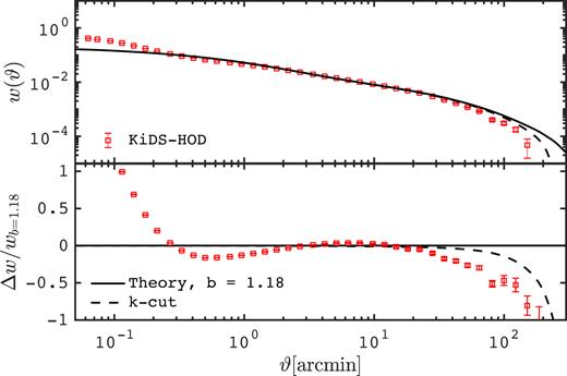
Upper: angular correlation function of the KiDS-HOD mocks compared to the predictions, assuming a galaxy bias of bKiDS = 1.18. The mocks are averaged from 100 lines of sight, their error bars are on the mean. This measurement has not yet been carried out in the KiDS-450 data. Lower: fractional difference with respect to the predictions.
Since the number density of galaxies fluctuates between lines of sights, the distributions of the sources and of the lenses would both contribute to the covariance in a weak-lensing measurement. This would introduce an additional variance compared to a suite of mock catalogues all constructed with a fixed n(|$z$|), such as the KiDS-450 source catalogue presented in Section 3.1. Depending on the error analysis strategy, this additional variance might already have been included elsewhere, such that there is a risk of double counting that component to the uncertainty. This is why we advocate against using these KiDS-HOD mocks for cosmic shear covariance estimation.
We also want to stress that there is no guarantee that the (low-redshift) GAMA luminosity function is accurate once extrapolated to higher redshifts. This could have an impact on some science applications, but not if the requirements on the mocks are only to be realistic and representative, such as for the study of the neighbour-exclusion bias (see Section 5).
3.7 LSST-like HOD mocks
Although the KiDS-HOD mock presented in the previous section is designed to emulate current weak-lensing surveys, its galaxy number density is lower than the forecasted values of future surveys. Following the same procedure, we describe here a separate mock that can be used for upcoming experiments: we extend the GAMA HOD up to |$z$| = 3 and produce an LSST-like mock13 with the redshift distribution presented in the lower panel of Fig. 14. This corresponds to a magnitude-limited survey with a cut at mr = 26.8, and has a number density of ngal = 25.8 gal arcmin−2.
We observe that the redshift distribution is shifted to higher redshifts compared to the Chang et al. (2013) forecast, due to the difficulty to produce as many low-redshift galaxies as required by the forecasted n(|$z$|). This would require the SLICS to resolve lower mass haloes, or the HOD to populate each halo with more satellites, or even to include these missing objects as ‘field galaxies’, placed at random in the light-cones. It is not clear which of the above-mentioned methods would provide the most realistic mock data, hence we decided to simply extrapolate the GAMA HOD to larger redshifts and find the apparent magnitude cut that best reproduces the object density, at the cost of biasing the mean redshift towards higher values. Overlooking this difference, these LSST-like mocks are representative of what future lensing data might look like, and can be used to test different aspects of the weak-lensing analyses that require an HOD backbone construction (source–lens coupling, close neighbours studies, etc.). In particular, we use them in our analysis of the neighbour-exclusion bias in Section 5.
3.8 Preparing mocks for other surveys
HOD prescriptions similar to those presented in the preceding sections can be used in conjunction with the halo catalogues to generate mock galaxy catalogues that emulate other surveys. This task can be made easier when the data selection strategy resembles that of a surveys for which mocks are already available. For example, the galaxy selection of the 2-degree Field Lensing Survey LRG sample (Blake et al. 2016a, 2dFLenS) is very close to the BOSS CMASS and LOWZ targets, with the main difference being a lower redshift completeness (Blake et al. 2016a). We hence do not need to construct a separate 2dFLenS mock sample, as it is possible to match the density of the data simply by randomly downsampling the BOSS mocks by 50 per cent. This approach has been used in Blake et al. (2016a) and Amon et al. (2018a).
Our HOD method could be used to construct mock data that resemble the DES lens sample (the redMaGiC sample, see Rozo et al. 2016), the WiggleZ spectroscopic galaxy sample (Drinkwater et al. 2018) or upcoming data from LSST14 or DESI15, as they become available.
3.9 Random catalogues
When measuring clustering in configuration space (with i.e. the Landy–Szalay estimator described in equation 2), a ‘random’ catalogue must be provided. Extra care must be taken to ensure that the random catalogue reproduces the n(|$z$|) and the 2D geometry of the data (or mocks), otherwise the estimator is no longer unbiased, and can contain significant systematic features. The density of the randoms is typically increased compared to the data, while the mask and survey boundaries are preserved. It has become common for public releases of clustering data to also provide a set of random catalogues tailored for the survey, and we describe in this section how we construct a similar set of randoms to be used with our simulated data products.
This is not as straightforward as it seems, owing to the fact that the SLICS simulations are produced from the multiple plane approximation (see Section 2.2). The 3D volume that ends up in the light-cone is not a cone or a pyramid, but a sequence of steps. It is essential that the randoms follow this 3D selection function inherent in the mocks. Also, since the randoms must be tailored to the mock data for which we wish to measure |$w$|(ϑ), they follow the n(|$z$|) from the mock surveys (and not the n(|$z$|) from the data).
We populate the randoms with 10 times the density of the mock data, and distribute the galaxies randomly within the pixels of the 100 deg2 light-cone (what we call the ‘ray-tracing’ coordinate frame). We finally transform these positions into ‘clustering coordinates’, a procedure that imparts the 3D geometry of the SLICS light-cones (see Appendix C for details on these two coordinate frames). We produce randoms for the CMASS, LOWZ, GAMA, and KiDS-HOD mocks, as well as for the |$z$| = 0.2 halo sample used in Fig. 4. These catalogues contain three quantities per object: (xclustering, yclustering, |$z$|spec), and are used in all |$w$|(ϑ) measurements presented in this paper.
3.9.1 Data products: galaxy catalogues
We provide the following galaxy catalogues:
KiDS-450 and KiDS-450-dense source galaxies, whose positions are placed at random in the light-cone (see Section 3.1);
LSST-like source galaxies, whose positions are placed at random in the light-cone (see Appendix A1);
CMASS, LOWZ, and GAMA spectroscopic lens galaxies, whose positions emerge from the HODs (see Sections 3.3–3.5);
KiDS-HOD and LSST-like HOD galaxies, whose positions emerge from the HODs (see Sections 3.6–3.7).
Random catalogues for clustering measurements with the CMASS, LOWZ, GAMA, and KiDS-HOD catalogues.
Additionally, we provide mock KiDS-450 observations covering the full mosaics, with mock galaxies placed at the exact same location as in the data. This additional mock is meant to be used primarily for peak statistics (as in Martinet et al. 2017) or other measurements sensitive to variations in source number density, and is described in Appendix A3.
3.10 Summary of known limitations
Numerical simulations, including all those listed in Table 1, always have built-in limitations that must be documented and acknowledged, especially when choosing the regime where the mocks are accurate and suitable for their science case. It is sometimes possible to forward model these limitations in a comparison between mock measurements and predictions, as for the case of mass resolution or finite-box effect. When this is possible, the observed mismatches are significantly reduced and can be ignored, especially when using the mocks for the calibration of estimators. However, fully accounting for these systematic effects is generally less obvious, for example for the estimation of covariance matrices, as discussed in HvW15. It is advisable then to exclude the elements of the data vectors for which the contamination level is important.
We list in this section all the known limitations from the SLICS mock catalogues that might or might not affect the analyses they are used for. These were previously discussed in the main text, and we strongly recommend that the users carefully read them in order to make precise statements about their measurements from the SLICS simulations.
There are no neutrino nor baryon feedback mechanisms: these mocks emulate a post-recombination universe in which all matter behaves as collisionless dark matter, with the imprint from the baryonic acoustic oscillations.
The particle mass resolution is |$2.88\times 10^9 \ h^{-1}\, \mathrm{M}_{\odot }$|, and haloes made of less than 100 particles are not fully resolved. This incompleteness is visible from the halo mass function, in Fig. 2, and could be inconsistent with some data samples that have a significant fraction of these low-mass haloes.
Finite resolution affects small angles (i.e. ϑ ≲ 1 arcmin in ξ+ at |$z$| ∼ 0.5, and ϑ ≲ 5 arcmin in ξ−). For the |$w$|(ϑ) measurement, this effect is degenerate with the non-linear halo bias that occurs at small scales. Generally, k modes smaller than |$2.0 \ h\, {\rm Mpc}^{-1}$| are well resolved.
Finite-box effects affect large angles (i.e. ϑ ≳ 1 deg in |$w$|(ϑ) and ϑ ≳ 0.5 deg in ξ+(ϑ)). These can be identified and modelled from predictions in which k modes larger than |$2\pi /(505\ h^{-1}\, {\rm Mpc})$| have been removed. The sampling variance extracted from the SLICS mocks should also be scaled using this modelling, as shown in HvW15.
The correlation across mass sheets has been explicitly broken, hence any 3D measurement should be performed only inside individual lens sub-volumes. We refer the reader to the values of |$z$|s in Table 2 in order to split the mock data in a manner that is insensitive to this. The data should then be split in the same way for consistency.
Although the n(|$z$|) and ngal of the KiDS-450 mocks match the data without the ZB cuts, discrepancies are observed in tomographic analyses (see Table 3). In that case, the n(|$z$|) still matches the data by construction, but ngal does not. Since this can be critical to many analyses, we recommend to use the KiDS-450-dense mock instead, then downsample the catalogues to recover the ngal from the data in whatever ZB slice is being analysed.
We have only measured the angular correlation function in broad redshift bins. Finer tomographic binning may reveal larger discrepancies.
Clustering measurements in our mocks are generally in close agreement with the data, but the linear bias sometimes differs by about 10 per cent. This is partly caused by differences in cosmology, which affects the clustering. We nevertheless recommend to consider and propagate these differences in data analyses, possibly by rescaling the mock measurements.
In the GAMA mocks, the K-corrections are degenerate with the redshift evolution of the luminosity function. We calibrate these together to empirically reproduce the n(|$z$|) given an apparent magnitude cut. However, the underlying luminosity function in the mocks might no longer be a good match to that of the data without the K-correction.
Satellite galaxies are placed according to spherical NFW profiles. We have decided not to use the triaxial profiles as there is no strong consensus that sub-haloes necessarily trace the dark matter. Additionally, the HOD prescriptions are calibrated assuming spherical NFW, which could make the interpretation less accurate. However, this means that the galaxy–galaxy lensing signal from the satellites is weaker than in the data, in which many satellite galaxies are believed to reside in sub-haloes/cores.
The concentration parameter is allowed to vary in order to maximize the agreement with the data in clustering measurements. This means that a detailed study of the one halo term – i.e. precise reconstruction of the halo profiles – might differ between the data and the mocks.
The inertia matrix provided by our halofinder is not very accurate since no phase-space cleaning has been applied before measuring this quantity. Certainly, the shapes are not reliable for haloes made of less than 400 particles, possibly more.
Despite these limitations, the SLICS mocks stand out as a particularly useful tool for combined probe studies involving weak lensing and remains accurate within the dynamical range listed above.
4 COMBINED-PROBE ANALYSES
Different cosmological probes are sensitive to different redshifts and/or dynamical ranges of the underlying large-scale structure formation. Differences in instruments and measurement strategies also mean that the systematic effects are typically distinct and uncorrelated. Combinations of probes at the data vector level exploit these advantages and offer complementary cosmological information and opportunities for self-calibration (see van Uitert et al. 2018; Joudaki et al. 2017; DES Collaboration et al. 2017, for recent combined-probes analyses). Control samples such as the SLICS are critical for the estimation of the correlation between the elements of the combined-probe data vector.
In the next sections, we first carry out a galaxy–galaxy lensing measurement in the mocks by combining our KiDS-450 source catalogues with different spectroscopic lens catalogues, comparing our results with measurements from the data. We then construct a larger data vector by adding (1) the clustering of the lenses and (2) the cosmic shear of the sources. We present the full covariance matrix of this combined data vector as a demonstration of what can be achieved with the SLICS.
4.1 Galaxy–galaxy lensing
We compare in Fig. 16 the ΔΣ(R) signal extracted from the KiDS-450 mock sources around the CMASS/LOWZ/GAMA targets, with the measurements from data presented in Amon et al. (2018a). To further ease the comparison with the measurements of |$w$|(ϑ) for these three mock surveys presented in Figs 9, 10, and 12, it is convenient to note that at their mean redshift (〈|$z$|〉 = 0.58, 0.32, 0.25), the angles subtended by the comoving size R = 1.0 h−1 Mpc are respectively 2.4, 3.9, and 4.8 arcmin.
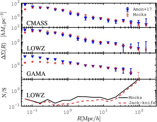
Upper three panels: differential surface mass density, ΔΣ, as measured in the KiDS-450 and CMASS/LOWZ/GAMA mocks, and compared to the measurement from the data by Amon et al. (2018a). The error bars on the mocks are on the mean, while that on data are from the mocks, scaled to the overlapping survey areas. Lowest panel: comparison between the error obtained from the mock covariance about the LOWZ × KiDS-450 measurement, and the JK estimate from the data.
The mocks and data agree within 1σ over a range of scales, however some discrepancies are observed. There is a noticeable difference in the signal at small angular scales for the GAMA survey, which is sourced by the implementation of the satellites in the mocks. Whereas the satellite galaxies in the data are believed to be highly correlated with sub-haloes (Velliscig et al. 2017), the satellites in the mocks are placed at random positions within a NFW profile (see Section 3.2), which destroys the satellite contribution to the galaxy–galaxy lensing signal. The LOWZ and CMASS mocks are less affected by this missing signal because of the smaller satellite fraction, compared to GAMA.
In absence of an ensemble of mock data, the errors on galaxy–galaxy lensing measurements are often estimated from analytical calculations that neglect the sampling variance, or from bootstrap or JK resampling of the data, which are generally accurate at small scales but perform less well at larger angles (see fig. 5 in Viola et al. 2015, for a comparison between these methods). Galaxy–galaxy lensing analyses interested in intrahalo properties need not to worry about this, but the same cannot be said about measurements that target the two-halo term, e.g. to constrain the galaxy bias.
The SLICS simulations are ideal to test the accuracy of these assumptions, since the error estimated from them contains both the shape noise and the sampling variance. A comparison between the SLICS and an analytical covariance is presented in Brouwer et al. (2018). We show here, in the lowest panel of Fig. 16, a comparison between the error on ΔΣ(R) obtained from the mocks in a LOWZ × KiDS-450 analysis, versus a JK estimate from the data. Both error estimates are normalized by the data signal to improve the readability, and their measurements of the noise-to-signal ratio agrees to within 10 per cent at the smallest scales shown here, but differ by up to a factor of two for R > 0.7h−1 Mpc.
A clear asset of the SLICS mocks is that they can provide error estimates even for surveys of smaller area (e.g. GAMA), where internal resampling is not reliable. One can also inspect with these mocks the relative contributions to the covariance from the shape noise and the sample variance, and/or combine the data vectors with other cosmological probes, as shown in the next section.
4.2 Covariance for 3 × 2 point data vectors
We present here the covariance matrix of a mock measurement similar in nature to that presented in van Uitert et al. (2018) and DES Collaboration et al. (2017), which combined three measurements of two-point correlation functions related to the foreground matter field. The data vector we analyse here consists of the ξ±(ϑ) cosmic shear data points measured from the KiDS-450 mock sources selected with 0.5 < ZB < 0.7 (presented in Section 3.1), the angular correlation function |$w$|(ϑ) measured from the LOWZ mock spectroscopic survey (Section 3.4) and the galaxy–galaxy lensing signal measured from their combination (Section 4.1). In the latter case, the source galaxies are not binned in ZB, and the signal is promoted from γt(ϑ) to ΔΣ(R) when compared to the two data analyses mentioned above.
We merge the mock data vector from each line of sight as X = [ξ+(ϑ), ξ−(ϑ), |$w$|(ϑ), ΔΣ(R)] and compute the full covariance matrix from 844 lines of sight with equation (8). We present the results in Fig. 17, normalized such that the diagonal is equal to one. The different blocks represent distinct components of the combined data vector, separated by thick black lines. We use a large number of bins in order to highlight the structure of the matrix, however most of the points are highly correlated; far fewer points are required to capture the same information content.
![Cross-correlation coefficient, $r_{ij} = {Cov}_{ij}/\sqrt{{Cov}_{ii}\, {Cov}_{jj}}$, for a combined-probe measurement involving cosmic shear ξ±(ϑ) from the KiDS-450 mocks, galaxy clustering $w$(ϑ) from the LOWZ mocks, and galaxy–galaxy lensing ΔΣ(R) from the combination of both. The cosmic shear segments of the data vector represent a single tomographic bin of the KiDS-450 mock data, selected with ZB ∈ [0.5 − 0.7]. The sources are not binned in the galaxy–galaxy lensing signal. Shape noise is included in the lower triangle part of this matrix, which explains why the off-diagonal components of the lensing data are suppressed compared to the upper triangle part.](https://oup.silverchair-cdn.com/oup/backfile/Content_public/Journal/mnras/481/1/10.1093_mnras_sty2319/1/m_sty2319fig17.jpeg?Expires=1750214237&Signature=qIXykm5hYb239dLcz7pnV-zYF6GIAEAR~kopVfFAHWCvOLTR0D9WPZsrxAUzWb3l7H1c8rBokcswp~AmasvGMikTKwIRpyFsfTUnhwfFzn02VJ48JBrMLQ0Pdl~DPYoFo-G8RQatjJkff1gh1lquG3Xs~tVsSoFPeHCgWdqygKxaXYz7RpdFmnKutkSx6DwWAWSxkswnrv2kdNRV-McVdvwAZQzT9joDqNSnVwVHv-AGWM-Gc8w8qzaD0okE785YZxblriFi-XRAdQZWjDK~uw-6lQ3Mwa1qbXgKdEUqgQ~tJupdZ2Wlei4nAK8J5E6kSWIcG4pJ9sOlaBAOfbbp1Q__&Key-Pair-Id=APKAIE5G5CRDK6RD3PGA)
Cross-correlation coefficient, |$r_{ij} = {Cov}_{ij}/\sqrt{{Cov}_{ii}\, {Cov}_{jj}}$|, for a combined-probe measurement involving cosmic shear ξ±(ϑ) from the KiDS-450 mocks, galaxy clustering |$w$|(ϑ) from the LOWZ mocks, and galaxy–galaxy lensing ΔΣ(R) from the combination of both. The cosmic shear segments of the data vector represent a single tomographic bin of the KiDS-450 mock data, selected with ZB ∈ [0.5 − 0.7]. The sources are not binned in the galaxy–galaxy lensing signal. Shape noise is included in the lower triangle part of this matrix, which explains why the off-diagonal components of the lensing data are suppressed compared to the upper triangle part.
The lensing data used in this calculation include shape noise as an option, which downweights the off-diagonal components of the normalized matrix when turned on (see the lower triangle part of Fig. 17). Even in this case, it is possible to observe some structured correlation in most blocks, although the noise level on individual elements is significant. The noise-free case is shown in the upper triangle part of the matrix in Fig. 17, where we can distinguish significant amounts of cross-correlation between most blocks.
The covariance matrix presented here is only one example of a 3 × 2 point data vector that can be formed from the SLICS, and it is straightforward to expand on this and include other data types such as RSDs, CMB lensing, void lensing, or lensing peak count, just to name a few. In some cases, a combined-probe covariance matrix can be estimated analytically, which provides an opportunity to validate the two approaches. Indeed, the halo model offers a prescription to compute this quantity via the trispectrum (Takada & Jain 2009; Krause & Eifler 2017). Some measurements however are harder or currently impossible to integrate in this framework (RSDs, void lensing, peak counts, non-linear transforms, etc.), but are fully accessible with the SLICS mocks. The caveat, of course, is that the covariance estimated from the mocks will be at a fixed cosmology, and subject to a limited precision due to the finite number of mocks. Lastly, as mentioned in the Introduction, the estimate will be biased low due to the missing SSC term. In practice, this term can be evaluated with response functions from ‘separate universe’ simulations (Li et al. 2014), by comparing the results to simulations with larger volumes (e.g. the HSC mocks presented in Table 1) or from Gaussian realizations. In van Uitert et al. (2018), it was shown that the SLICS mocks contain some contribution to the SSC term from the simulation volume outside of the light-cone. The missing contribution would inflate the cosmic shear error by 10–70 per cent depending on the angular scale, but has no effect on the galaxy–galaxy lensing error. This is indeed an important ingredient that must supplement the covariance estimate extracted from the SLICS.
5 NEIGHBOUR-EXCLUSION BIAS ON COSMIC SHEAR
In this second part of the paper, we make use of the 120 KiDS-HOD and LSST-like HOD mocks described in Sections 3.6 and 3.7 to revisit a selection effect related to close neighbours that was first identified in Hartlap et al. (2011). The general idea is that isophote overlap makes the positions and shape measurement generally difficult, inaccurate or biased for these objects. For this reason, they are either fully removed or downweighted, depending on the analysis strategy, and this choice introduces a selection effect that is not random on the sky due to clustering. Indeed, galaxy clusters have the highest density of objects, hence they have higher chances to contain close neighbours and blended objects. This effect exists even in smaller systems, since any background galaxy that exactly aligns with a foreground massive dark matter halo is obscured by the central galaxy. This translates into an effective downsampling of the foreground overdensities compared to the rest of the sky, a bias that affects the cosmic shear signal. As a corollary, voids in the foreground have lesser chances of containing close neighbours and are thus given more weight.
Hartlap et al. (2011) studied this effect using the Millennium Simulations, and reported an impact of a few per cent to tens of per cent on cosmic shear measurements, depending on the scales, redshifts, and definition of ‘close galaxy pairs’ that are excluded. MacCrann et al. (2017) studied this effect – which they referred to as the blend-exclusion bias – in a cosmic shear analysis of the DES-Science Verification (SV) data targeted at small scales. They estimated its impact from image simulations and provided a physically motivated model of this bias, and finally investigated different degeneracy directions, notably with the sum of neutrino mass and with baryon feedback parameters. In this paper, we term this effect the neighbour-exclusion bias on the weak-lensing signal, following the terminology of Samuroff et al. (2018)17, in which a number of neighbour-induced biases have also been studied in the context of cosmic shear measurements with the first year of DES data. Their strategy was different as they used pairs of simulations with and without clustering, and merged multiple shear biases into a scale-dependent multiplicative correction term. This method is accurate, but its calibration also depends on the survey depth, redshift distribution, and on the exact galaxy sample used. In the end, mock data such as the SLICS are required for validating the framework.
We build on these preceding results by exploring the impact on different cosmic shear analysis pipelines with shallow and deep mock data, with an eye on the signal in cross-tomographic bin combinations and on the residual effect at large angles. We focus at first on the (shallower) KiDS-450 survey, and discuss the (deeper) LSST-like survey afterward.
5.1 Measurement from mocks
We start by identifying close pairs in the full KiDS-HOD mocks with a KDTree (Friedman, Bentley & Finkel 1977) algorithm.18 During this stage, we use different definitions of close pairs: objects separated by less than: 1.0, 2.0, 3.7, and 5.0 arcsec on the sky. These exclusion angles are meant to represent the variable shape measurement quality confronted to realistic seeing conditions, and the largest three of these are taken from Hartlap et al. (2011) for validation and cross-reference; the 1.0 arcsec separation targets future surveys. We next adopt two strategies to deal with the close pairs we have found. Either we reject the faintest of the two galaxies in a pair – we refer to this technique as ‘FAINT’ – or we remove both galaxies from the catalogues – we refer to this as ‘BOTH’. These two cases emulate different pipelines currently used in weak-lensing analyses.
Removing close pairs from the catalogues has two effects: (1) it modifies the mean redshift distribution, preferentially removing high-redshift galaxies since their mean angular separation is smaller due to their larger distance from us, and (2) it preferentially reduces the number of galaxy pairs aligned with foreground structures, which is the anisotropic selection effect at the core of this study. The first effect does no harm to a data analysis as it is effectively a downsampling of the data: as long as the estimated final n(|$z$|) is accurate, the inferred cosmology will not be affected by this. The second effect is more problematic however as it correlates with the foreground matter distribution. This is similar to the selection effect described in Simet & Mandelbaum (2015), who examined the impact of cluster obscuration on cluster mass reconstruction with stacked shear and magnification signals (see also Hoekstra et al. 2015).
To isolate the neighbour-exclusion bias, we need to factor out the first effect. Following the ‘FIX’ criterion (Hartlap et al. 2011), we proceed as follows:
Find and remove close pairs from the KiDS-HOD mocks. The outcome of this are ‘filtered catalogues’. We repeat this for the range of exclusion angles and for the two selection criteria, BOTH and FAINT.
Split the original and filtered catalogues in four tomographic bins. For this work, we reduce the complication arising from photometric error and split our data according to their true redshift: |$z$|spec ∈ [0.1 − 0.3], [0.3 − 0.5], [0.5 − 0.7], and [0.7 − 0.9].
Measure the |$\widehat{\xi ^{ij}}_{\pm }(\vartheta)$| signal from the original and filtered catalogues, in all pairs of tomographic bins (i, j).
Measure the original and filtered n(|$z$|), and compute the associated theoretical predictions |$\xi ^{ij}_{\pm }(\vartheta)$|.
We show in Fig. 18, the ratio between the redshift distributions of the full sample, with and without filtering, for the FAINT and BOTH techniques and for the different exclusion angles. As redshift increases, all curves first show that the filtering removes an increasing number of galaxies, which simply reflects the fact that more galaxies are contained within the same solid angle. This trend starts to reverse beyond redshift |$z$| = 0.7, where the n(|$z$|) of the KiDS-HOD mocks begins to fall off (see the top panel of Fig. 14). The BOTH filter rejects approximately twice as many objects as the FAINT as expected; the FAINT filter preferentially rejects objects at higher redshift that appear dimmer, and preserves almost all low-redshift objects.

Effect of the close pair selection on the number density of objects in the 120 KiDS-HOD mocks galaxy catalogues, presented as the ratio between the filtered and original N(|$z$|). Different colours represent different opening angles in the close pairs selection criteria, solid lines represent the FAINT rejection scheme, and dashed lines show BOTH. Approximately twice as many objects are rejected in the latter case.
Our measurements of |$\beta _{+}^{ij}(\vartheta)$| and |$\beta _{-}^{ij}(\vartheta)$| are presented in Figs- 19 and 20, respectively. We see that larger exclusion angles exhibit larger effects, as expected from the larger fraction of objects with close neighbours. These results are in excellent agreement with the equivalent results from Hartlap et al. (2011, see their ‘FIX’ method). We additionally find that higher redshift measurements are more affected by this selection bias due to the higher fraction of close pairs, and that cross-tomographic signals are impacted as well. Because the neighbour-exclusion bias mainly occurs at small scales, the measurement of |$\widehat{\xi }_-$| suffers from a stronger bias than |$\widehat{\xi }_+$|, at fixed angle.

Effect of the close-pair selection on ξ+ signal in the KiDS-HOD mocks galaxy catalogues. Left- and right-hand panels show the FAINT and BOTH prescriptions, respectively. y-axes show β+, defined in equation (21), while x-axes show the separation angle in arcminutes. Different colours represent different opening angles used in the definition of close pairs. Upper left to lower right show the results for tomographic bins with increasing redshift. Dashed black lines represent the best fit from equation (22). Right-hand panels: same as left, but for the BOTH prescription. The KiDS-450 cosmic shear analyses included angular scales down to 0.5 arcmin in their analysis (Hildebrandt et al. 2017), while the smallest angles included in the DES cosmic shear measurement went from 7 arcmin at lower redshifts to 3.5 arcmin at higher redshifts (Troxel et al. 2017).

Same as Fig. 19, but this time for β−. Note the change in y-scaling. The KiDS-450 cosmic shear analyses included angular scales down to 4.2 arcmin in their analysis, while the DES cosmic shear measurement excluded scales smaller than 70 arcmin at low redshift and 35 arcmin at high redshift.
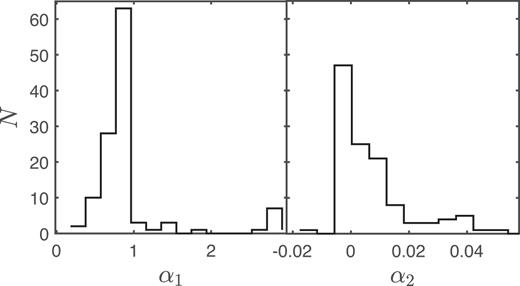
Distributions of the best-fitting parameters α1,2, which model the neighbour-exclusion bias according to equation (22). These histograms could be used as informative priors on these two parameters in a procedure that marginalizes over this selection effect.
Additionally, given that the shapes of β± are similar to those arising from the impact of baryon feedback on the matter density field (Semboloni et al. 2011), this contribution must be included in the interpretation of the measured baryon feedback parameters, something omitted in previous analyses (H17, Harnois-Déraps et al. 2015) and forecasts (Foreman, Becker & Wechsler 2016), but first pointed out in MacCrann et al. (2017). Alternatively, marginalizing over the baryon feedback parameters and/or over the reduced-shear model should, at the same time, mitigate this selection effect, whose amplitude is lower than some of the most extreme feedback models.
We now investigate the importance of this effect on two current weak-lensing measurement strategies.
5.2 Neighbour-exclusion bias in a lensfit-like pipeline
As a first example, we examine the KiDS-450 analysis pipeline of H17. It first uses SExtractor (Bertin & Arnouts 1996) to provide a catalogue of deblended objects. These catalogue entries are then passed to lensfit (Miller et al. 2007, 2013), which performs the galaxy shape measurement on the images with as few cuts as possible on the selected objects, as described in H17. lensfit masks neighbouring objects when measuring each target object, but as this process does not fully correct for light leaking outside the neighbours’ masked regions, a ‘contamination radius’ statistic, to test for the presence of close neighbours, is also measured, calculating the distance to the nearest detected neighbour (Miller et al. 2013). If the contamination radius is less than 4 pixels, the object is flagged and excluded from the analysis. The flagging system is described in Miller et al. (2013), and captured by the FITCLASS flag in the KiDS-450 data and image simulation catalogues. For the KiDS-450 cosmic shear analysis, a stricter criterion of 4.25 pixels was employed to minimize additive bias (see Appendix D in H17). In this method, the effect of blending at a given centroid-to-centroid separation strongly depends on the galaxy sizes and is found to preferentially remove fainter galaxies. With a pixel size of 0.214 arcsec, this means that the blending strategy here corresponds closely to the FAINT technique, with full blending occurring approximately at 0.9 arcsec.
A second selection is at play in this shape measurement strategy: the presence of a close neighbour may affect the weight assigned to that galaxy: close neighbours tend to be measured as being more elliptical and to have higher weights than they would if they had been measured in isolation. Although these objects are not excluded from the analysis, their detection rate and weight are affected by the presence of neighbours, which can be related to an ‘effective’ exclusion angle. In order to study this, we make use of image simulations similar to those on which lensfit was calibrated for the KiDS-450 cosmic shear analysis (Fenech Conti et al. 2016). These improved simulations are augmented with realistic input galaxy properties which are inferred from the Hubble Space Telescope COSMOS data. This current study, however, uses only a subset of the full suite designed for shear calibration; we investigate the effect of bad and good seeing conditions, but do not include variations in the lensing shear or galaxy rotations. These are required for a full shear calibration, but have minimal impact on close pairs selection. We run the lensfit shape measurement tool on these simulations and constructed object catalogues based on the input (the ‘true’ objects) and output (the ‘lensfit measurement’ of these objects). For each input object, the catalogues contain the input and detected positions and magnitudes, a shape weight, a ‘source-type’ flag (FITCLASS) that identifies stars, galaxies, blends, badly measured objects, etc., and a flag for objects that were not matched to the simulation input. Our matching condition requires that the centroid of an observed object resides within a 3 pixel radius of an input centroid.
We construct our baseline catalogue by first removing all the input stars, then applying an mr < 24.5 cut such as to mimic the observed data. Ignoring this step would overestimate the effect by artificially boosting the depth. We next construct the lensfit measurement catalogue by requiring FITCLASS = 0 and by rejecting unmatched galaxies. We then count the close pairs that are present in the ‘true’ and ‘filtered’ catalogues (optionally summing the lensfit weights, in the second case) as a function of separation, and finally take the ratio between the two measurements. We normalize the ratio to unity at 6 arcsec, where filtering should be minimal. This ratio is shown in the lower panel of Fig. 22, where we see that close pairs are in fact unaffected by close-neighbours selection for angular scales larger than 3 arcsec, but reliable shape measurements for more than half the close pairs are not produced by the pipeline below 1.8 arcsec. This means that the KiDS-450 measurement strategy can be representatively identified as the dark blue lines in Figs 19 and 20, in the left-hand panels describing the FAINT technique.

Upper: ratio between the number of pairs in the DES-SV catalogue with and without applying the sextractor flag. Lower: ratio between the number of pairs in the image simulations that mimic the KiDS-450 data, with and without including the effect of the lensfit measurement.
In the cosmic shear analysis of H17, the |$\widehat{\xi }_+$| and |$\widehat{\xi }_-$| measurements extend from ϑ > 0.5 and 4.2, respectively. From Figs 19 and 20, we can therefore expect the KiDS cosmic shear signal to be affected by the neighbour-exclusion bias by less than a percent.
5.3 Neighbour-exclusion bias in an ngmix-like pipeline
As a second example, we examine one of the pipelines used by the DES Collaboration on their SV data, presented in Becker et al. (2016) and re-examined in MacCrann et al. (2017). In their strategy, the ngmix shape measurement pipeline with meta-calibration (Sheldon & Huff 2017) was run on all objects that passed the sextractorFLAG_i<2 cut, which rejected both blended objects identified by sextractor. Once that was done however, all shapes were given the same weight. This is similar in nature to the filter BOTH presented in Section 5.1. The question now is to find the effective exclusion angle at which the filter operates.
We measure this by running our close-pairs finder algorithm on the public SV catalogue,19 with and without applying the FLAG_i<2 filter. We then compare the number of close pairs in the upper panel of Fig. 22, again normalizing the ratio to unity at the largest angle. The effect of the selection becomes apparent already at 4 arcsec, and by 2.5 arcsec almost half of the pairs are filtered out. Note that this measurement differs in nature from that carried out on the KiDS image simulation, since we do not know the ‘input’ here, but only the objects detected by sextractor. This explains why the ratio does not converge to zero at zero lag: many pairs separated by less than 1 arcsec were not even detected to start with due to obscuration by the foreground member.
According to this figure, this measurement strategy has a close pair definition bracketed between 2 and 3.7 arcsec, plotted as blue and green symbols on Figs 19 and 20. This is in excellent agreement with the results on the impact of close pairs reported in MacCrann et al. (2017) for the same DES-SV data, which provides robust validation of both approaches.
We emphasize that the results quoted in this section cannot be directly applied to the DES data, since this survey has a different depth and density than the KiDS-HOD mocks analysed here. Instead, one should think of our results as the outcome of a DES-like analysis (notably the shape measurement method) performed on KiDS-like data. The technique is general though, and hence some conclusions can be reached for the DES-year1 cosmic shear analysis of Troxel et al. (2017). While the neighbour-exclusion bias significantly deviates from unity at small scales, their cosmic shear analysis is protected against this effect for three reasons: (1) their upgraded meta-calibration strategy no longer requires the FLAG_i<2 cut, reducing even more the size of the effect, (2) they have folded this effect into their new shear calibration (Samuroff et al. 2018), and (3) they applied aggressive angular cuts on the measurements: in order to minimize the contamination from baryon feedback, they excluded angular scales smaller than 3.5 (7.0) arcmin in the highest (lowest) tomographic bin for ξ+, and 35 (70) arcmin in the highest (lowest) tomographic bin for ξ−. As seen in the right-hand panels of Figs 19 and 20, the amplitude of the neighbour-exclusion bias on these angular scales is less than a percent.
5.4 Future surveys
The upcoming weak-lensing experiments such as LSST and Euclid are expected to achieve sub-percent precision on cosmological parameters from cosmic shear measurements. The neighbour-exclusion bias must therefore be accurately captured in order to interpret the measurement correctly. At KiDS depth, this effect is mostly significant on smaller angular scales, but a residual effect propagates to all scales. We illustrate this in Fig. 23, which zooms-in on the fit function described by equation (21), over the range 5 < ϑ < 100 arcmin. The different colours match the separation angles presented in Fig. 19, and the four panels show β± for the FAINT and BOTH methods. All tomographic bins are overplotted. Even at large angular separations, these models are mostly consistent with the measurements. The agreement is not perfect in all tomographic bins, but the trends are captured with enough accuracy to support our result: the effect on ξ+ is below 0.3 per cent at all scales, but ξ− can be affected by 0.5 per cent at 20 arcmin.
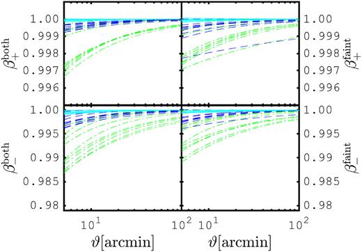
Zoom-in on the neighbour-exclusion bias model at large angles in mock data at KiDS-depth, estimated from the fit function (equation 21). Upper and lower panels show β+ and β−, respectively; right- and left-hand panels show FAINT and BOTH methods, respectively. The different colours (cyan, blue, and green) match the different separation angles presented in Fig. 19 (1, 2, and 3.7 arcsec, respectively), and the different lines of the same colour show the fits from the 10 panels in that figure.
We investigate this further with the LSST-like HOD mocks presented in Section 3.7, where the number density is almost four times higher than the KiDS-HOD mocks, with a redshift distribution that now extends to |$z$| = 3. We carry out a single 2D cosmic shear analysis over 20 of these mocks, and extract the neighbour-exclusion bias for the BOTH and FAINT cases, assuming that rejection of close neighbours occurs at 1.0 or 2.0 arcsec separation. The results, presented in Fig. 24, indicate that the ξ+ and ξ− measurements are affected by half a per cent and up to 2 per cent, respectively, when the exclusion angle is set to 2 arcsec. If we reduce the exclusion angle down to 1 arcsec separation, then the ξ+ and ξ− measurements are affected by 0.2 and 0.5 per cent, respectively.

Neighbour-exclusion bias measured from the LSST-like HOD mocks with 1 and 2 arcsec exclusion angles, compared to the best-fitting models estimated from the KiDS-HOD reported in Fig. 23. Upper and lower panels show β+ and β−, respectively; and left- and right-hand panels show FAINT and BOTH methods, respectively.
Also shown in Fig. 24 are the best-fitting models estimated from the shallower KiDS-HOD mocks, previously reported in Fig. 23. We clearly see that the LSST-like data points are systematically lower than the KiDS-HOD best-fitting lines. We can further read off from this figure that, at fixed close-pairs model and exclusion angle, the neighbour-exclusion bias affects more severely our LSST-like mock data compared to the KiDS-HOD mock data, by about a factor two, which means that if we are to marginalize over the neighbour-exclusion bias using α1, 2 as nuisance parameters, then their priors need to be revisited.
There is a key caveat in our analysis which stems from our choice to populate the mocks with unit weight sources that match the effective number density of the KiDS and LSST surveys (8 and 26 gal arcmin−2, respectively), rather than matching the raw number density with non-unit weights. The number of close pairs in the raw data is larger, hence the neighbour-exclusion bias is expected to be larger. Furthermore our study does not include any dependence on the size distribution that slowly varies with redshift and magnitude. The technique presented here will therefore be extended in future analyses to extend the complexity of the mock source sample in order to determine a more accurate amplitude for the neighbour-exclusion bias. For future high-precision surveys, we would advocate marginalizing over a model given by equation (22) using informative priors on the two nuisance parameters from a mock galaxy analysis.
6 CONCLUSIONS
We describe a suite of numerical simulation products tailored for the estimation of covariance matrices in combined-probe analyses involving weak-lensing data from the KiDS. Many of these have already been used to date, hence the first part of this paper serves as the main reference for the description of the methodology and performance of the mock data used in these analyses. More specifically, we generate 844 fully independent realizations of mock lensing data that emulate the KiDS-450 and an LSST-like survey described in Chang et al. (2013), in individual patches of 100 deg2 each. In the same simulated light-cones, we also include mock catalogues that emulate spectroscopic galaxy surveys such as GAMA, CMASS, LOWZ, and 2dFLenS, as well as CMB lensing convergence maps. Used in conjunction with the lensing mocks, these different simulation products can serve for pipeline validation and uncertainty estimation in combined-probe analyses involving e.g. cosmic shear, galaxy–galaxy lensing estimators, galaxy clustering, RSDs, and their cross-correlation with the CMB lensing data. We quantify the accuracy of the galaxy catalogues by comparing the redshift distributions and clustering with the data they are meant to emulate; we reach 20 per cent agreement or better on the two-point correlation function |$w$|(ϑ) over a range of dynamical scales, with residual differences partly caused by our choice of cosmological parameters. At small angular scales, the variance obtained from the mock clustering and galaxy–galaxy lensing measurements are consistent with JK estimations of the error; we identify from the mocks scales where the latter becomes unreliable. We generate a 3 × 2-point function data vector that includes cosmic shear, lens clustering, and galaxy–galaxy lensing measurements, and present an estimation of the covariance matrix for these combined probes.
In the second part of the paper, we demonstrate how these mocks can be used to estimate the neighbour-exclusion bias at KiDS and LSST depth, inspired by the early work of Hartlap et al. (2011). For this particular science case, we produce two additional suites of mock data, in which both the lenses and the sources catalogues are extracted from an HOD prescription. These are meant to be representative of the KiDS-450 and LSST surveys, and include realistic levels of source–lens coupling, photometric uncertainty, galaxy clustering, and redshift distributions. We identify galaxies with close neighbours in our mock lensing data with four different exclusion angles, and investigate two methods to cope with them, representative of the shape measurement techniques used in the DES and in the KiDS-450 data. We compare the cosmic shear signal with and without the filtering of these close pairs, in the context of a four-bin tomographic analysis. We find a redshift dependence in the selection effect: the neighbour-exclusion bias is larger at higher redshift due to the increase in number of objects at fixed solid angle. At KiDS-depth and assuming poor seeing conditions blurring objects separated by less than 5 arcsec, the impact on the ξ+ measurement is of the order of a few percent, while it reaches up to 10 per cent for the same angular scales for ξ− (see Figs 19 and 20). In all cases, the angular dependence of this effect has a simple shape that we model with a two-parameter function (see equation 22). We measure the distribution of these two parameters over all tomographic bins, which could serve as a prior in an MCMC marginalization pipeline for current surveys. This prior will however need to be revisited for future deeper surveys using the methodology outlined in this paper.
We investigate the sensitivity of current cosmic shear analyses to this selection bias by identifying the filtering technique that best matches the data measurement procedure. The ngmix pipeline uses sextractor flags to reject blended objects, which effectively suppresses most pairs separated by less than 2.5 arcsec, as verified on the DES-SV data. Given the conservative cuts that were applied on the angular scales, we find that this ξ± measurement is affected by less than a percent. The DES year 1 results are further protected since the updated meta-calibration method does not require the cut of sextractor flags. The KiDS-450 pipeline uses the lensfit shape measurement tool, which returns a shape weight that is affected by the proximity of close neighbours. We measure the effective close-pairs exclusion radius from KiDS-like image simulations and find that more than half the close pairs are rejected when separated by less than 1.8 arcsec. The KiDS-450 cosmic shear analysis extended to 0.5 arcmin in ξ+ and 4.2 arcmin in ξ−, at which scales the amplitude of the neighbour-exclusion bias is always less than a percent.
We next measure this bias in deeper and denser mock data in a non-tomographic setup, and find that the amplitude of the effect is about twice the size measured from the shallower KiDS-HOD mocks. For future lensing surveys like LSST, the neighbour-exclusion bias needs to be understood with high accuracy since it is degenerate with baryon feedback parameters (MacCrann et al. 2017) and can be mostly addressed with an angle-dependent shape calibration technique (Samuroff et al. 2018). In any case, these future measurements will need to be calibrated against numerical simulations such as those presented in this paper, possibly upgraded with actual images for each object.
The SLICS mocks can find a number of applications in data analyses, for estimator validation and calibration, in the data processing, for estimation of covariance matrices in combined-probe measurements, for studies of statistical properties of covariance and likelihood functions, or for the investigation of systematic effects. Many of these applications are relatively new and would require further exploration in order to reach the level of accuracy and control required for future lensing surveys. To encourage and accelerate this progress, we make all simulation products publicly available at http://slics.roe.ac.uk.
ACKNOWLEDGEMENTS
The HOD calculations used in the paper inherits from the code written by Marcello Cacciato, who also provided many advices on general HOD strategies. Shadab Alam and Chris Blake also contributed to these discussions, which helped us in deciding what strategy best suited our needs. We would like to thank Ian Fenech Conti, and Ricardo Herbonnet for their help with the image simulations, Alexander Smith for sharing the details of his GAMA HOD prescription, Joe Zuntz for providing the LSST n(|$z$|) and for his insights on the DES shape measurement strategy, and the anonymous referee for their useful comments. This work also benefitted from discussions about blending with Javier Sanchez and Joe Zuntz. We would like to acknowledge the input of many users that have tested the different simulation products and provided invaluable feedback that helped us finding bugs and making the mock products easier to use, notably Chris Blake, Massimo Viola, Edo van Uitert, Marika Asgari, India Rose Friswell, Harry Johnston, Nicolas Martinet and Axel Buddendiek, Elena Sellentin, and Chien-Hao Lin. We thank Martin Kilbinger for help with the athena correlation function measurement software and the nicaea theoretical modelling software, Mike Jarvis for maintaining treecorr, and Joe Zuntz for help with CosmoSIS.
JHD is supported by the European Commission under a Marie-Skłodowska-Curie European Fellowship (EU project 656869). CH and AA acknowledge support from the European Research Council under grant number 647112; AA is further supported by a LSSTC Data Science Fellowship. VD acknowledges the Higgs Centre Nimmo Scholarship and the Edinburgh Global Research Scholarship. AK and HHo acknowledge support from the Netherlands Organisation for Scientific Research (NWO) Vici grant 639.043.512. RN acknowledges support from the German Federal Ministry for Economic Affairs and Energy (BMWi) provided via DLR under project no. 50QE1103. LvW is supported by the NSERC of Canada. HHi is supported by an Emmy Noether grant (No. Hi 1495/2-1) of the Deutsche Forschungsgemeinschaft. LM acknowledges support from STFC grant ST/N000919/1.
Computations for the N-body simulations were performed in part on the Orcinus supercomputer at the WestGrid HPC consortium (www.westgrid.ca), in part on the GPC supercomputer at the SciNet HPC Consortium. SciNet is funded by: the Canada Foundation for Innovation under the auspices of Compute Canada; the Government of Ontario; Ontario Research Fund – Research Excellence; and the University of Toronto. The post-processing calculations were mainly carried out on the Cuillin cluster at the Royal Observatory of Edinburgh, which is run by Eric Tittley.
The mock data presented in this paper are calibrated against observations from KiDS, GAMA, and BOSS. This KiDS data are based on data products from observations made with ESO Telescopes at the La Silla Paranal Observatory under programme IDs 177.A-3016, 177.A-3017, and 177.A-3018.
GAMA is a joint European-Australasian project based around a spectroscopic campaign using the Anglo-Australian Telescope. The GAMA input catalogue is based on data taken from the Sloan Digital Sky Survey and the UKIRT Infrared Deep Sky Survey. Complementary imaging of the GAMA regions is being obtained by a number of independent survey programmes including GALEX MIS, VST KiDS, VISTA VIKING, WISE, Herschel-ATLAS, GMRT, and ASKAP providing UV to radio coverage. GAMA is funded by the STFC (UK), the ARC (Australia), the AAO, and the participating institutions. The GAMA website is http://www.gama-survey.org/. Also based on observations made with ESO Telescopes under programme ID 177.A-3016.
Funding for SDSS-III has been provided by the Alfred P. Sloan Foundation, the Participating Institutions, the National Science Foundation, and the U.S. Department of Energy Office of Science. The SDSS-III web site is http://www.sdss3.org/. SDSS-III is managed by the Astrophysical Research Consortium for the Participating Institutions of the SDSS-III Collaboration including the University of Arizona, the Brazilian Participation Group, Brookhaven National Laboratory, Carnegie Mellon University, University of Florida, the French Participation Group, the German Participation Group, Harvard University, the Instituto de Astrofisica de Canarias, the Michigan State/Notre Dame/JINA Participation Group, Johns Hopkins University, Lawrence Berkeley National Laboratory, Max Planck Institute for Astrophysics, Max Planck Institute for Extraterrestrial Physics, New Mexico State University, New York University, Ohio State University, Pennsylvania State University, University of Portsmouth, Princeton University, the Spanish Participation Group, University of Tokyo, University of Utah, Vanderbilt University, University of Virginia, University of Washington, and Yale University.
We would finally like to thank McGill University for its hospitality, where an important part of the HOD code development was made.
All authors contributed to the development and writing of this paper. The authorship list is given in three groups: the lead author (JHD), followed by two alphabetical groups. Members of the first alphabetical group carried out key infrastructure work specifically for this paper. Members of the second alphabetical group provided proprietary data central to this work, or contributed to the analysis.
Footnotes
This is not an exhaustive list of all public mock weak-lensing data, but instead a subset that shows the diversity of the available tools.
Note that the setup described here has changed since HvW15, in which the light-cones had an opening angle of 60 deg2 with 60002 pixels.
Planck lensing package: pla.esac.esa.int/pla/#cosmology.
This halo property refers to its rank in a mass-ordered halo catalogue, where the lowest rank corresponds to the most massive halo.
ATHENA: www.cosmostat.org/software/athena/.
NICAEA: www.cosmostat.org/software/nicaea/.
We have also experimented with the implementation from Manera et al. (2013), an HOD calibrated on the DR10 BOSS data release. This other calibration prefers higher number densities, but the resulting clustering amplitude is too low compared to the DR12 data, hence we adopted the Alam et al. (2017b) HOD model.
BOSS-DR12: https://data.sdss.org/sas/dr12/boss/lss/.
Note that the HOD parameters in equations (6) and (7) are named differently in the papers where they are first introduced. There is nevertheless a one-to-one correspondence between our notation (Mcut, σ, M1, κ, α) and that used in Smith et al. (2017): |$(M_{\rm min}, \sigma _{{\rm log} M}, M_0, M_{1}^{\prime }, \alpha)$|.
The K-correction that is discussed here enters in the conversion between absolute and apparent magnitude. It is not to be confused with the k-mode correction mentioned previously, which has to do with missing Fourier modes in a finite volume simulation box.
GAMA:www.gama-survey.org.
Note that this mock product differs from the other LSST mock presented in Appendix A1, in which the n(|$z$|) is imposed and galaxy positions are placed at random in the light-cones.
LSST: https://www.lsst.org.
DESI: desi.lbl.gov.
We use the galaxy–galaxy lensing notation from Dvornik et al. (2018): ΔΣcom(R) and Σcr, com are sometimes labelled ΔΣ(R) and Σcrit, respectively. This is to be distinguished from measurements in ‘proper’ distance, which we do not use in this section.
The neighbour-exclusion bias is the exact same phenomenon that was coined the blend-exclusion bias in MacCrann et al. (2017), but this latter name can lead to a confusion since by definition, ‘blended’ galaxies refer to nearly complete overlap of two objects that makes them nearly undistinguishable. These normally appear as a single catalogue entry with high shape noise. Our naming captures the fact that this selection effect operates mainly on pairs of galaxies that are close but distinguishable.
We used the python module scipy.spatial.KDTree.
DES-SV data: https://des.ncsa.illinois.edu/releases/sva1/doc/gold.
Because of these discontinuities in redshift, the full 3D correlation is broken across these boundaries, which will affect 3D clustering measurement such as ξ(r) or |$w$|(rp). This does not prevent the application of the SLICS to such data analyses, but might shape the data vector such as to impose similar selection cuts in the data.
REFERENCES
APPENDIX A: ADDITIONAL SOURCE GALAXY CATALOGUES
A1 Mock LSST-like source galaxies

Redshift distributions used for the 10 tomographic bins of the LSST-like source catalogues, assuming the survey specifications presented in Chang et al. (2013) with α = 1.25, β = 1.0, and |$z$|0 = 0.5.
We compute the shear two-point correlation function from these mocks using equation (4), and the results are shown in Fig. A2 for all combinations involving the first five tomographic bins, and without shape noise. We recover the results presented in Section 3.1 and in HvW15, namely that the angular scales comprised in the range [1–50] arcmin in ξ+ are generally modelled to better than 5 per cent, however smaller scales suffer from limits in particle mass resolution, while large scales are affected by the finite simulation box size.

Cosmic shear measured from the first five tomographic bins of the LSST-like source mocks, ignoring shape noise. The y-axis shows the fractional difference between the measurements of ξ+ (left) and ξ− (right) from the mocks and the predictions obtained from nicaea with the input cosmology and n(|$z$|). The x-axis shows the angular separation ϑ in arcminutes. Error bars show the error about the mean, and the tomographic bins are labelled on the sub-panels.
A2 Source galaxies with clustering at fixed bias
In addition to the random position and HOD approaches, we have produced mock galaxy catalogues in which the position of the galaxies trace the underlying dark matter with a controlled bias. We do this by sampling the projected 2D density mass sheets δ2D(χl, θ) at random such that the density distribution of galaxies in each redshift slice is proportional to the mass distribution projected within the slice. This has the advantage that it contains lens clustering, but the bias is a controlled parameter, as opposed to being redshift, scale, and mass dependent. This is helpful when comparing measurements to theoretical models that assume linear bias (see H17, van Uitert et al. 2018, for two applications of these mock data).
A3 Source galaxies with positions set by data
We have developed another type of mock catalogues also based on the SLICS light-cones, and in which the position of the galaxies exactly match those of the KiDS-450 data. The prime application of this approach is to reproduce the observed variation in source density, which modulates the local noise properties and affect statistics such as weak-lensing peak counts (for a detailed discussion on the importance of this, see Martinet et al. 2017).
Since we cannot capture all the data in one light-cone, we break the observed sky coverage into 100 deg2 patches, and tile the mocks into a mosaic, as illustrated in Fig. A3. The five KiDS-450 fields are decomposed into 17 ‘mock regions’, shown as red boxes. Unfortunately, the KiDS mosaic is not efficiently decomposed into 10 × 10 regions, which is why these 450 deg2 of data take significantly more than 4.5 mock light-cones to be covered. However, many mock regions contain very little data and we could recycle some unused coverage, keeping this to a minimum in order to avoid unphysical correlations. After this tiling technique, the position of every galaxy in the KiDS-450 data passing a 0.1 < ZB < 0.9 cut is matched to a pixel in one of 13 SLICS light-cones, organized into 17 regions. To be clear, there is no correlation between the location of these mock galaxies and the large scale structure from the mocks.

Tiling configuration of the 17 SLICS simulations onto the 5 KiDS patches. The red squares represent the area of individual light-cone. The axes are in the xy coordinate frame of the masks, in units of arcminutes. Each black point corresponds to a galaxy in the KiDS catalogue.
The next step is to assign a shear to these objects, which requires knowledge of their redshift in the simulation. To achieve this, we draw a |$z$|spec value from the DIR n(|$z$|) and use this redshift to interpolate the two shear components from the shear planes described in Section 2.2, at the pixel location. We include in the mock the original coordinates of the galaxy, the coordinate in the mock light-cone, the original observed ellipticity, the shear extracted from the SLICS, the ZB and |$z$|spec redshifts, as well as the shape weight and the Field ID. These quantities, summarized in Table A1, are all required by peak statistic analyses such as the one carried out in Martinet et al. (2017). We generated with that method a total of 67 independent mock replicas of the KiDS mosaic, based on tiling 871 SLICS light-cones. Note that the n(|$z$|) is similar but not exactly identical to that of the ‘main’ KiDS-450 sample (described in Section 3.1), causing variations of order 10 per cent on the cosmic shear signal.
Additional content of the mock galaxy catalogue at the KiDS-450 galaxy positions – all columns from the KiDS-450 source catalogues described in Table 4 are included as well. The XY are in the coordinate frame of the mask, and related to the RA–Dec. with the WCSTools sky2xy or xy2sky.
| Content | Units | Description |
|---|---|---|
| X | ||
| Y | ||
| |$\Big \rbrace$| Sky coordinates | ||
| w | lensfit weight from the data | |
| FieldPos | Telescope pointing |
| Content | Units | Description |
|---|---|---|
| X | ||
| Y | ||
| |$\Big \rbrace$| Sky coordinates | ||
| w | lensfit weight from the data | |
| FieldPos | Telescope pointing |
It is important to note that the simulated data contained in different mock regions (the red boxes in Fig. A3) are not correlated, as they originate from different light-cones. In contrast, these correlations exist in the data, which means that care must be taken to avoid being affected by this difference. For example, one should not compute correlation functions on the full mock mosaic, otherwise the broken correlation across the regions will result in a significantly lower signal, compared to both the data and the predictions. Instead, analyses should be carried out within the individual mock regions. The peak statistics analysis described in Martinet et al. (2017) is protected against this, since the shear peaks are found from an aperture mass algorithm that works on individual camera pointings that each cover about 1 deg2.
APPENDIX B: MORE DETAILS ON THE GAMA HOD
We describe in this appendix the ingredients that allow us to model the GAMA mock survey including the redshift and luminosity dependence of the HOD parameters. We closely follow the modelling of Smith et al. (2017), but include some details relevant to this mock production. This HOD is also used in the production of the KiDS-HOD and LSST-like HOD mocks, described in Sections 3.6 and 3.7, respectively. First, as noted explicitly in equation (11), the relation between luminosity and halo mass changes with redshift, and its evolution is characterized by the parameter Q. Second, the dependence on luminosity requires the construction of relations between L, Mmin, and |$M_{1}^{\prime }$|, which are given by the same functional form as equation (11), but replacing some terms. To establish the |$M_{1}^{\prime }(L)$| relation, we replace (Mh, L⋆At, Mt, αM) by (|$M_{1}^{\prime }(L), 3.70\times 10^9 \ h^{-2}L\odot , 4.78\times 10^{12}\ h^{-1}\, \mathrm{M}_{\odot }, 0.306$|), while for the Mmin(L) we replace them by (|$M_{\rm min}(L), 3.92\times 10^9 \ h^{-2}\, \mathrm{L}_\odot , 3.07\times 10^{11}\ h^{-1}\, \mathrm{M}_{\odot }, 0.258$|).

Luminosity function of the GAMA mocks that includes redshift evolution of the HOD and K-correction. The black line represents the effect of removing the mr < 19.8 requirement, keeping otherwise all galaxies up to |$z$| = 0.5.
APPENDIX C: Ray tracing versus clustering coordinates
As mentioned earlier, the SLICS mocks are based on the flat sky multiple plane geometry (described in Section 2.2), which is an excellent approximation for current cosmic shear analyses that probe the lensing signal out to angular scales as large as 10 deg. By construction, the cosmological volume that contributes to a pixel |${\boldsymbol \theta }$| in the ith mass plane |$\delta _{\rm 2D}(z^i_{\rm l},{\boldsymbol \theta })$| comes from the projection of half the simulation box (with thickness |$L_{\rm box}/2 = 256.5 \ h^{-1}\, {\rm Mpc}$|) along one of the Cartesian axis. Assuming the flat sky and far-field limits, this axis is therefore identified as the radial direction and used thereafter in the assignment of both redshifts and comoving distances for haloes and galaxies living in the light-cones. This is no longer accurate for near-field objects, or for projected quantities involving less than five parallel planes, especially when looking at clustering of these low-redshift lenses, and requires a correction that we describe here. Since we know the exact 3D position of each halo and galaxy from the simulation, we can compute the correct angular coordinates of the objects (i.e. projecting radially, not along a Cartesian axis), and store these quantities as well.
For the sake of precision, there is thus a need for two coordinate systems to describe the lenses in our simulations. We define the ‘ray-tracing’ coordinate, or |${\boldsymbol \theta }_{\rm ray-tracing}$|, as the mass projection coordinate. That is, all objects that contribute to the same pixel in the mass map (or shear map) share the same |${\boldsymbol \theta }_{\rm ray-tracing}$| coordinate. Their true coordinate, which we refer to as the ‘clustering coordinate’, or |${\boldsymbol \theta }_{\rm clustering}$|, can be significantly different on account of the differences in the projection, especially for lower redshift objects. This is illustrated by the left-hand panel of Fig. C1. The thin horizontal lines represent the 18 lens planes listed in Table 2, each subtending 10 deg and 7745 pixels in both direction. The vertical red ‘sticks’ show how volume elements are projected at their centres, as part of the mass plane construction. These red sticks represent the clustering coordinates, sampled at 13 angles, and clearly show the discontinuities20 that occurs between the mass planes.

Illustration of the two coordinate systems needed by the mock data. Left: the data points in each red ‘stick’ represent example of objects that share the same |${\boldsymbol \theta }_{\rm ray-tracing}$| coordinates, even though their |${\boldsymbol \theta }_{\rm clustering}$| coordinates differ. In the multiple lens technique, the photon trajectories descend along red sticks that are connected by a common black line. They are then assigned to pixels with coordinate |${\boldsymbol \theta }_{\rm ray-tracing}$|, traced by the black lines. In the far-field limit, the red and black align. Right: the |${\boldsymbol \theta }_{\rm clustering}$| coordinate of the same red points, as seen from lines of constant |${\boldsymbol \theta }_{\rm ray-tracing}$|. In this frame, the |${\boldsymbol \theta }_{\rm clustering}$| coordinates extend outside the 10 × 10 deg2 patch.
The black lines in the left-hand panel of Fig. C1 show the |${\boldsymbol \theta }_{\rm ray-tracing}$| coordinates of the same objects, which are continuous at all redshifts. These coordinates are not physical, and rather serve as a label that connects haloes with mass sheets. Note that both coordinate systems coincide on the lens planes and at the very centre of the light-cone. Their difference increases for objects that approach the edges of the light-cone, the junction redshifts, and at lower redshift in general. We show in the right-hand panel of Fig. C1 the |${\boldsymbol \theta }_{\rm clustering}$| and |${\boldsymbol \theta }_{\rm ray-tracing}$| coordinates of the same red sticks, but as seen in the |${\boldsymbol \theta }_{\rm ray-tracing}$| frame. The black curved lines from the left-hand panel become straight lines of constant RA, while the large differences between the two coordinate systems become even more apparent.
We emphasize again that |${\boldsymbol \theta }_{\rm clustering}$| corresponds to the actual position of the object in the simulation, and hence should be used for clustering measurements such as |$w$|(ϑ), |$w$|(rp), void-finding, etc. In contrast, |${\boldsymbol \theta }_{\rm ray-tracing}$| traces the projection used in the making of the mass sheets and should be used for lensing measurements (γt, ξ±, etc.). As an example, we show in Fig. C2, the angular correlation function |$w$|(ϑ) of all redshift |$z$| ≡ 0.22 haloes, previously presented in Fig. 4. For this measurement to be accurate, it is critical to have random catalogues that properly capture the properties of the survey in absence of clustering. We discuss this further in the context of our light-cone geometry in Section 3.9. Shown in red is the clustering measurement from |${\boldsymbol \theta }_{\rm clustering}$|, i.e. at their correct positions, compared with theoretical predictions that assume a bias of 1.0. In black is the same measurement carried out with |${\boldsymbol \theta }_{\rm ray-tracing}$| instead, which shows clear unphysical features. This illustrates the importance of using the correct column in the mocks.

Same as Fig. 4, but here including the measurements from the two coordinates described in the main text: |${\boldsymbol \theta }_{\rm clustering}$| (red) and |${\boldsymbol \theta }_{\rm ray-tracing}$| (blue). Clustering measurements must use the former, lensing measurements the latter.
For example, in a mock joint-probe analysis involving cosmic shear from the KiDS-450, galaxy–galaxy lensing from KiDS-450 combined with CMASS, and clustering of CMASS, the measurement would involve:
|${\boldsymbol \theta }_{\rm ray-tracing}$| in the KiDS-450 mocks for the cosmic shear measurement,
|${\boldsymbol \theta }_{\rm ray-tracing}$| in the KiDS-450 mocks and |${\boldsymbol \theta }_{\rm ray-tracing}$| in the CMASS mocks for the tangential shear measurement, and
|${\boldsymbol \theta }_{\rm clustering}$| in the CMASS mocks for the |$w$|(ϑ) measurement.
To make this easy for the user, we provide both coordinates in our halo and galaxy catalogues. We also include simple codes to switch between these two coordinate systems, made available with the simulation products.
APPENDIX D: FLAT SKY APPROXIMATION
In this appendix, we verify the validity of the flat sky assumption in the SLICS simulations. The 3D coordinates of the galaxies/haloes in the simulation box are first given in Cartesian coordinates, then transformed into angles and redshifts. In this process, the third Cartesian axis is assumed to be equivalent to the radial direction, which is only valid in the far-field limit. The two angles are not affected by this approximation, but the redshift is. For example, a galaxy located at a large angle (for example at X = Y = 5 deg) and very close to the front of the simulation box (for example at 15 h−1 Mpc) appears at redshift |$z(\chi = 15 h^{-1}\, {\rm Mpc}) = 0.005$|. However, its true distance to the observer is χ = 15.11 h−1 Mpc, which is a sub-percent effect. Moreover, only a minor fraction of objects at very low redshifts will suffer from error larger than 1 per cent coming from the flat sky approximation.
To show this, we populate a light-cone with a number of objects covering all angles and redshifts present in the mocks. We then calculate the fractional effect of the approximation on the computed redshift at all these coordinates and show the results in Fig. D1. We recover that only the lowest redshifts are affected by this, which are heavily downweighted in any lensing analysis, hence conclude that this is not an issue for the science cases targeted by the SLICS simulations.

Fractional error between flat sky and curved sky redshifts, for objects at different positions on the light-cone. Objects shown with redder lines are closer to the edges of the simulation box, where the correction is more important. The dashed line marks the 1 per cent error.
