


ABSTRACT
Cosmic rays are usually assumed to be the main ionization agent for the interior of molecular clouds, where UV and X-ray photons cannot penetrate. Here, we test this hypothesis by limiting ourselves to the case of diffuse clouds and assuming that the average cosmic ray spectrum inside the Galaxy is equal to the one at the position of the Sun as measured by Voyager 1 and AMS-02. To calculate the cosmic ray spectrum inside the clouds, we solve the 1D transport equation taking into account advection, diffusion, and energy losses. While outside the cloud particles diffuse, in its interior they are assumed to gyrate along magnetic field lines because ion-neutral friction is effective in damping all the magnetic turbulence. We show that ionization losses effectively reduce the CR flux in the cloud interior for energies below ≈100 MeV, especially for electrons, in such a way that the ionization rate decreases by roughly two order of magnitude with respect to the case where losses are neglected. As a consequence, the predicted ionization rate is more than 10 times smaller than the one inferred from the detection of molecular lines. We discuss the implication of our finding in terms of spatial fluctuation of the Galactic cosmic ray spectra and possible additional sources of low-energy cosmic rays.
1 INTRODUCTION
As molecular clouds (MCs) shield quite effectively both UV photons and X-rays (Krolik & Kallman 1983; Silk & Norman 1983; McKee 1989), cosmic rays (CRs) seem to be the only capable agents to ionize their interior. It is for this reason that CRs are believed to play an essential role in determining the chemistry (Dalgarno 2006) and the evolution of these star-forming regions (e.g. Wurster, Bate & Price 2018). Recent observations (Caselli et al. 1998; Indriolo & McCall 2012, see Padovani, Galli & Glassgold 2009 for a review) have suggested that the CR-induced ionization rate decreases for increasing column density of MCs, and it varies from around ≈10−16 s−1 for diffuse MCs down to ≈10−17 s−1 for dense ones.
The ionization rates measured in MCs are tentatively interpreted as the result of the penetration of ambient CRs into clouds (Padovani et al. 2009). Thus, in order to model this process and test this hypothesis one needs to know: (i) the typical spectrum of low-energy CRs in the Galaxy, and (ii) the details of the transport process of CRs into MCs. Remarkably, the spectra of both proton and electron CRs in the local interstellar medium (ISM) at least down to particle energy of a few MeVs are now known with some confidence because of the recent data collected by the Voyager probe at large distances from the Sun (Stone et al. 2013; Cummings et al. 2016). Whether or not such spectra are the representative of the average Galactic spectra, especially for MeV CRs, is still not clear (this is an old-standing issue, see e.g. Cesarsky 1975). However, the analysis of gamma-rays from MCs (e.g. Yang, de Oña Wilhelmi & Aharonian 2014) seems to indicate that at least the spectrum of proton CRs of energy above a few GeV is quite homogeneous in our Galaxy.
Several theoretical estimates of the CR-induced ionization rate in MCs have been performed over the years. The first attempts were done by simply extrapolating to low energies the spectra of CRs observed at high energies, without taking into account the effect of CR propagation into clouds (e.g. Hayakawa, Nishimura & Takayanagi 1961; Tomasko & Spitzer 1968; Nath & Biermann 1994; Webber 1998). Such estimates provide a value of the CR ionization rate that is known as the Spitzer value and is equal to ≈10−17 s−1. This value is an order of magnitude below the observed data for diffuse clouds and roughly similar to the value found in dense ones.
Later works included also a treatment of the transport of CRs into MCs and considered the role of energy losses (mainly ionization) suffered by CRs in dense and neutral environments. A natural starting point is to consider the scenario that maximizes the penetration of CRs into clouds. This was done, most notably, by Padovani et al. (2009), who assumed that CRs penetrate MCs by moving along straight lines. A more realistic description, however, should take into account the fact that the process of CR penetration into MC is highly non-linear in nature. This is because CRs themselves, as they stream into the cloud, generate magnetic turbulence through streaming instability (Wentzel 1974). The enhanced magnetic turbulence would, in turn, induce an increase in the CR scattering rate on to MHD waves, which regulate their flux into clouds. The exclusion mechanism of CRs from MCs due to this type of self-generated turbulence was first studied in the pioneering works of Skilling & Strong (1976), Cesarsky & Völk (1978), and Morfill (1982), while recent studies in this direction include the works by Morlino & Gabici (2015), Schlickeiser, Caglar & Lazarian (2016), and Ivlev et al. (2018). Nevertheless, none of the models including a more thorough treatment of the effect of CR penetration into clouds have been confronted with the available observational data.
The main goal of this article is to fill this gap and provide the first comparison between the theoretical predictions from detailed models of CR transport and the measured values of the CR ionization rate in MCs, with a focus on to diffuse ones. We anticipate here the main results obtained in the following: the intensity of CRs in the local ISM as revealed by Voyager measurements is too weak to explain the level of ionization rate observed in clouds. Possible solutions to this problem include the presence of another source of ionization or a non-uniform intensity of low-energy CRs throughout the Galaxy.
The paper is organized as follows: in Section 2, we describe a model for the penetration of CRs into clouds. The model is then used to derive the spectra of CR protons and electrons inside MCs (Section 3) and to predict the CR ionization rate, which is then compared to available data (Section 4). We discuss our results and conclude in Section 5.
2 A MODEL FOR THE PENETRATION OF COSMIC RAYS INTO DIFFUSE CLOUDS
The penetration of CRs into diffuse clouds is described by means of a 1D transport model, where CRs are assumed to propagate only along magnetic field lines. This is a good description of CR transport provided that (i) the propagation of particles across magnetic field lines can be neglected, and (ii) the spatial scales relevant to the problem are smaller than, or at most comparable to the magnetic field coherence length in the ISM (here, we assume ≈50−100 pc). Both conditions are believed to be often satisfied and thus this setup was commonly adopted in the past literature to describe the penetration of CRs into MCs (e.g. Skilling & Strong 1976; Cesarsky & Völk 1978; Morfill 1982; Everett & Zweibel 2011; Morlino & Gabici 2015; Schlickeiser et al. 2016; Ivlev et al. 2018).
In the following, we describe an improved version of the model developed by Morlino & Gabici (2015), who considered a diffuse cloud of size Lc and uniform hydrogen density nH embedded in a spatially homogeneous magnetic field of strength B directed along the x-axis (see Fig. 1).
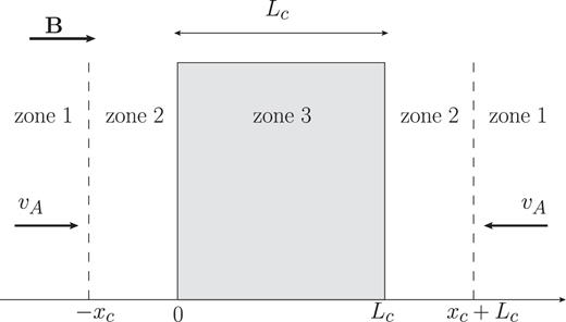
Setup of the problem. A cloud of size Lc is embedded in an homogeneous magnetic field of strength B directed along the x-axis. The direction of the Alfvén speed is also shown. See text for the definition of zone 1, 2, and 3, and of the diffusion scale xc.
A spatially uniform field in Zones 1–3 (see Fig. 1) is appropriate to describe diffuse clouds, but not dense ones (see the observational results reported in e.g. Crutcher et al. 2010) that, for this reason, are not considered in this paper. Note that, for simplicity, the transition from the low density and ionized ISM gas (of density ni) to the dense and neutral cloud environment (of density nH ≫ ni) is taken to be sharp and located at x = 0 and x = Lc. Morlino & Gabici (2015) limited themselves to consider the transport of CR protons only, while here we extend the analysis to include also CR electrons. Moreover, as discussed in the remainder of this section, we improve the description of the transport of CRs inside the cloud.
In the pioneering papers by Skilling & Strong (1976) and Cesarsky & Völk (1978), it was suggested that MCs may act as sinks for low-energy CRs. This is because low-energy CR particles lose very effectively their energy due to severe ionization losses in the dense gas of the cloud. In steady state, the rate at which CR particles are removed from the cloud due to energy losses has to be balanced by an incoming flux of CR particles entering the cloud (Skilling & Strong 1976; Morlino & Gabici 2015). The penetration of CR particles into the cloud is accompanied by the excitation of Alfvén waves due to streaming instability (Wentzel 1974). Such instability mainly excites waves propagating in the direction of the streaming of CRs. Therefore, a converging flow of Alfvén waves is generated outside the cloud (see Fig. 1). Once inside the cloud, Alfvén waves are damped very quickly due to ion-neutral friction (Zweibel & Shull 1982). Hence, following Morlino & Gabici (2015), we consider three regions (see Fig. 1):
Zone 1, located far away from the MC (x < −xc and x > xc + Lc), where the CR intensity is virtually unaffected by the presence of the cloud. As a consequence, in this zone the CR particle distribution function f(x, p) (p is the particle momentum) is roughly constant in space and equal to the sea of Galactic CRs f0(p). The quantity xc will be defined later.
Zone 2, located immediately outside the cloud (−xc < x < 0 and Lc < x < Lc + xc). In this zone, the CR particle distribution function is significantly affected by the presence of the cloud and is significantly different (i.e. smaller) than f0(p).
Zone 3, which represents the cloud (0 < x < Lc), and where particles suffer energy losses (mainly due to ionization).
The setup of the problem discussed above is intendedly simplified. A more realistic description of a cloud should include, between Zones 2 and 3, an envelope of atomic hydrogen characterized by a quite small column density of the order of few times 1020 cm−2 (see e.g. Snow & McCall 2006 for a review of cloud properties). Moreover, a smooth transition between the fully ionized and diffuse ISM and the dense and neutral MC should also be considered. In practice, the setup described in Fig. 1 can still be considered an appropriate description if the edge of the cloud (x = 0 and x = Lc) is defined as the position at which the ionization fraction of the gas is small enough to allow for a very effective damping of Alfvén waves due to ion-neutral friction.
As explained above, the waves propagate in opposite directions on the two sides of the cloud. This means that equation (1) is, strictly speaking, applicable only in the range x < 0 since the advection term would change the sign for waves propagating in the negative direction of the x-axis. Indeed, this complication could be overcome by solving the problem in the range x < Lc/2 only and adopting the symmetric condition introduced in Morlino & Gabici (2015) that gives f(x, p) = f(Lc − x, p). Also, we search here for steady-state solutions, and thus we set ∂f/∂t = 0.
To solve the problem, it is convenient to consider separately CRs of high and low energy, with E* being the energy defining the transition between the two domains (see Ivlev et al. 2018 for a similar approach). Following Morlino & Gabici (2015), E* is defined in such a way that particles with energy E > E* can cross ballistically the cloud without losing a significant fraction of their energy. If τl is the energy loss time of CRs inside the cloud (see Fig. 2), then the energy E* is obtained by equating τl with the CR ballistic crossing time |$\tau _c \sim L_c/\bar{v}(E_*)$|, where |$\bar{v}$| is the CR particle velocity averaged over pitch angle (the angle between the particle velocity and the direction of the magnetic field). Obviously, for E > E* the spatial distribution of CRs inside the cloud is, to a very good approximation, constant. It is important to stress that energy losses play an important role also for particle energies E > E* (no energy losses in a single cloud crossing), because such CRs are confined in the vicinity of the MC by the converging flow of Alfvén waves, and can thus cross and recross the cloud a very large number of times (for a more detailed discussion of this issue the reader is referred to Morlino & Gabici 2015).
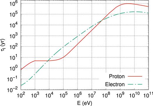
Energy loss time for CR protons and electrons in a cloud of density nH = 100 cm−3. The loss times are from Padovani et al. (2009).
2.1 High energies
As said above, equation (4) provides a general solution for spectrum of CRs with energy E > E*, or equivalently, of momentum larger than p > p*. The numerical values for the critical energy E* and momentum p* can be found from the expression τl(p*) ≃ 2Lc/|$v$|(p*), where |$v$|(p*) is the speed of a particle of momentum p* (here, we set |$\bar{v}=v/2$|). For a cloud of size Lc = 10 pc and nH = 100 cm−3 (or equivalently of column density |$N_{\text{H}_2}=n_\mathrm{ H}L_\mathrm{ c}=3.1 \times 10^{20}$| cm−2), we found p*,p ∼ 75 MeV/c and p*,e ∼ 0.34 MeV/c corresponding to a kinetic energy of E*,p ∼ 3.0 MeV and E*,e ∼ 0.1 MeV for protons and electrons, respectively.
2.2 Low energies
It is worth mentioning that equation (9) is not a formal solution of equation (2) because, in general, one would expect 〈cos ϑ〉 ≠ 1/2. However, we have checked the result obtained from equation (6) with the approximate solution obtained by the method of flux balancing (see section 2 in Morlino & Gabici 2015) and the two results match for particles with |$v$| ≫ |$v$|A.
3 COSMIC RAY SPECTRA IN DIFFUSE CLOUDS
In this section, we will use equations (4) and (9) to determine the spectrum of CR protons and electrons inside a given MC. In order to do so, we will need to specify the following:
the spectrum of CR protons |$f_0^p(p)$| and electrons |$f_0^e(p)$| far away from the cloud (Zone 1 in Fig. 1);
the column density |$N_{\mathrm{ H}_2}$| and the size Lc of the cloud;
the Alfvén speed |$v$|A in the medium outside the cloud (Zones 1 and 2).
As pointed out in Morlino & Gabici (2015), it is a remarkable fact that the spectrum of CRs inside the cloud does not depend on the CR diffusion coefficient (this quantity does not appear in neither equation 4 nor 9).

Parameters of the fits to the CR proton and electron intensity measured by Voyager 1 and AMS-02.
| Species | C (eV−1 cm−2s−1sr−1) | α | β | Ebr (MeV) |
|---|---|---|---|---|
| Proton | 1.882 × 10⁻⁹ | 0.129 | 2.829 | 624.5 |
| Electron | 4.658 × 10⁻⁷ | −1.236 | 2.033 | 736.2 |
| Species | C (eV−1 cm−2s−1sr−1) | α | β | Ebr (MeV) |
|---|---|---|---|---|
| Proton | 1.882 × 10⁻⁹ | 0.129 | 2.829 | 624.5 |
| Electron | 4.658 × 10⁻⁷ | −1.236 | 2.033 | 736.2 |
Results are shown in Fig. 4 for both CR protons and electrons, for a cloud of column density |$N_{\text{H}_2}=3.1\times 10^{21}$| cm−2 and for a value of the Alfvén speed of |$v$|A ≃ 200 km s−1. We assume a quite large value for the Alfvén speed to maximize the penetration of CRs into clouds. The reason for this assumption will become clear in the following. The three curves represent the spectrum of CRs far away from the cloud f0(E) = 4πj0(E)/|$v$|, the spectrum fb(E) at the cloud border (x = 0 and x = Lc), and the spectrum averaged over the cloud volume fa(E). At large enough energies, CRs freely penetrate clouds and the three spectra coincide. As noticed by Morlino & Gabici (2015), this is the case for particles that are not affected by energy losses during their propagation in zones 2 and 3 (see Fig. 1). For the cloud considered in Fig. 4 (|$N_{\text{H}_2} \sim 3.1 \times 10^{21}$| cm−3) and for a value of the magnetic field of 10 |$\mu$|G, this happens at Eloss,p ∼ 39 MeV for CR protons and Eloss,e ∼ 32 MeV for electrons (see equation 7 and related discussion in Morlino & Gabici 2015). Below these energies, the proton and electron spectra inside the cloud are suppressed with respect to f0, but in the energy range E*,p(E*,e) < E < Eloss,p(Eloss ,e), we still find that fb = fa. E*,p and E*,e have been defined at the end of Section 2.1. This fact can be easily undertood in the following way:
for proton (electron) energies larger than Eloss,p (Eloss,e) CRs freely penetrate the cloud, so that f0 = fb = fa;
for proton (electron) energies in the range E*,p < E < Eloss,p (E*,e < E < Eloss,e), particles suffer ionization energy losses, but this happens after they repeatedly cross the cloud. This implies that the CR spatial distribution inside the cloud is uniform, and thus f0 ≠ fb = fa;
for proton (electron) energies E < E*,p (E < E*,e), particles lose energy before completing a single crossing of the cloud, which implies that the spatial distribution of CRs inside the cloud is non-uniform, i.e. f0 ≠ fb ≠ fa.
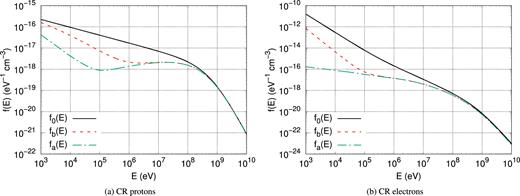
CR spectra for a cloud of column density |$N_{\text{H}_2}\sim 3.1\times 10^{21}$| cm−2 (corresponding to typical values of nH = 100 cm−3 and Lc = 10 pc). The left and the right figures are, respectively, spectra of protons and electrons. Also shown with the black solid curves are the ISM spectra given by equation (10).
In Fig. 5, we provide also a few spectra to show how our results depend on the exact value of the column density of the cloud. It is clear from the figure that the suppression of the CR spectra inside MCs is more pronounced for larger column densities. For very large column densities, approaching ∼1023 cm−2, the CR proton and electron spectrum is suppressed with respect to f0 up to quite large energies reaching the GeV domain.
Average spectra of CR protons (left-hand panel) and electrons (right-hand panel) inside clouds of different column densities as listed in the labels. The average ISM spectra of equation (10) are also shown with the black solid lines.
4 IONIZATION RATES
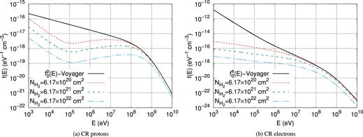
Fig. 6 shows the differential contribution to the ionization rate (|$E\mathop {}\!\mathrm{d}\zeta ({\text{H}_2})/\mathop {}\!\mathrm{d}E$|) for a few test clouds with column density 6.2 × 10²⁰, 6.2 × 10²¹, and 6.2 × 1022 cm−2 for both protons and electrons. This corresponds to an MC of size ∼10 pc with gas density of ∼20, 200, and 2000 cm−3, respectively. The differential ionization rates computed using the non-propagated Voyager spectra are also shown as the black lines. These results provide an indication for the range of particle energies that contribute to ionization the most. For the particular case considered here (CRs outside the cloud have a spectrum equal to that observed by Voyager), it is clear that the differential ionization rate peaks at about ≈100 MeV for both protons and electrons, with a quite weak dependence on the cloud column density.
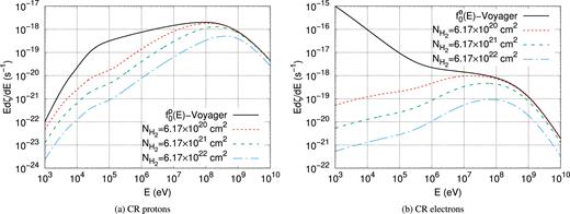
Differential ionization rate of both proton and electron CRs (left-hand and right-hand panels, respectively) at different column densities with the ISM spectra f0 assumed to be that from Voyager and AMS-02 fits. The black curves are the differential ionization rates obtained neglecting propagation and ionization losses into the cloud.
The dependence of the ionization rate with respect to the cloud column density predicted from our method is shown in Fig. 7, together with the observational data taken from Caselli et al. (1998), Williams et al. (1998), Maret & Bergin (2007), and Indriolo & McCall (2012). The ionization rates for protons and electrons (ζp(H2) and ζe(H2), respectively) are plotted together with the total ionization rate defined as ζ(H2) = ηζp(H2) + ζe(H2), where the factor η ≃ 1.5 accounts for the contribution to the ionization rate from CR heavy nuclei (Padovani et al. 2009).
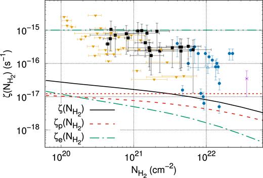
Ionization rate derived from Voyager spectra compared to observational data as a function of the column density. The two dot–dashed line and the dotted line correspond to the ionization rates of electrons and protons, respectively, neglecting the effects of propagation and ionization losses. Data points are from Caselli et al. (1998; filled circles), Williams et al. (1998; empty triangle), Maret & Bergin (2007; asterisk), and Indriolo & McCall (2012; the filled squares are data points, while the filled inverted triangles are upper limits).
It should be noticed that the results in Fig. 7 have been obtained under the assumption of a quite large value of the Alfven speed (approximately 200 km s−1). As said before, that was done to maximize the effect of the penetration of CRs into MCs. In fact, a more appropriate value would be about 60 km s−1, corresponding to a magnetic field strength of 3 |$\mu$|G and a density of ni ∼ 10−2 cm−3. If the calculation was done for such a value of the Alfven speed, the result of the ionization rate would be smaller by roughly a factor of 2.
Thus, it is evident from Fig. 7 that the predicted ionization rate fails to fit data, being too small by a factor of several tens at the characteristic column density of diffuse clouds (|$N_{\text{H}_2} \sim 10^{21}$| cm−2). It seems, then, that the intensity of CRs measured in the local ISM is by far too weak to explain the ionization rates observed in MCs. A discussion of this issue and possible solutions to such a large discrepancy will be provided in the final section of this paper. It has to be noticed, however, that the predictions presented in Fig. 7 are consistent with the upper limits on the ionization rate measured for a number of clouds (data points represented with the filled inverted triangles).
The range of column densities considered in Fig. 7 encompasses the typical values of both diffuse and dense clouds (a transition between the two regimes can be somewhat arbitrarily set at NH ≈ few 1021 cm−2 Snow & McCall 2006), while the model presented in this paper applies to diffuse clouds only. The propagation of CRs through large column densities of molecular gas may differ from the description provided in this paper mainly because large column densities are encountered in the presence of dense clumps, where the assumption of a spatially homogeneous distribution of gas density and magnetic field are no longer valid. The presence of clumps may affect CR propagation mainly in two ways:
Magnetic mirroring: The value of the magnetic field cannot be assumed to be spatially homogeneous in clumps, where it is known to correlate with gas density (Crutcher et al. 2010). The presence of a stronger magnetic field in clumps may induce magnetic mirroring of CRs, as investigated in Padovani & Galli (2011). This fact would lead to a suppression of the CR intensity and thus also of the ionization rate. This would further increase the discrepancy between model predictions and data;
Particle losses: Very dense clumps may act as sinks for CR particles. This happens when the energy losses are so effective to prevent CR particles to cross the clump over a time-scale shorter than the energy loss time. Such a scenario was investigated by Ivlev et al. (2018). Under these circumstances, a larger suppression of the CR intensity inside MCs is expected (energy losses are on average more intense), and this would also increase the discrepancy between data and predictions.
5 DISCUSSION AND CONCLUSIONS
The main result of this paper can be summarized as follows: If the CR spectra measured in the local ISM by the Voyager 1 probe are characteristic of the entire ISM, then the ionization rates measured inside MCs are not due to the penetration of such background CRs into these objects, and another source of ionization has to be found. This is a quite puzzling result, which necessarily calls for further studies. Several possibilities can be envisaged in order to explain the discrepancy between model predictions and observations. A non-exhaustive list includes
Better description of the transition between diffuse and dense media: At present, all the available models aimed at describing the penetration of CRs into MCs rely on the assumption of a quite sharp transition between a diluted and ionized medium, and a dense and neutral one. A more accurate description should consider a more gradual transition between these two different phases of the ISM. However, we recall that the simple flux-balance argument mentioned in Section 2 and discussed in great detail in Morlino & Gabici (2015) would most likely hold also in this scenario. It seems thus unlikely that a more accurate modeling could result in a prediction of ionization rates more than one order of magnitude larger than that presented here (as required to fit data);
Inhomogeneous distribution of ionizing CRs in the ISM: The assumption of a uniform distribution of CRs permeating the entire ISM could be incorrect. Fluctuations in the CR intensity are indeed expected to exist, due for example to the discrete nature of CR sources (see for example Gabici & Montmerle 2015, and references therein). However, gamma-ray observations of MCs suggests that such fluctuations are not that pronounced for CR protons in the GeV energy domain (Yang et al. 2014). Thus, fluctuations of different amplitude should be invoked for MeV and GeV particles;
CR sources inside clouds: The ionizing particles could be accelerated locally by CR accelerators residing inside MCs. Obvious candidate could be protostars, which might accelerate MeV CRs, as proposed by Padovani at al. (2015, 2016);
The return of the CR carrot? The existence of an unseen component of low-energy CRs, called carrot, was proposed a long time ago by Meneguzzi, Audouze & Reeves (1971) in order to enhance the spallative generation of 7Li, which at that time was problematic. Voyager data strongly constrain such a component, which should become dominant below particle energies of few MeV (the energy of the lowest data points from Voyager). Such a low-energy component could also enhance the ionization rate, as recently proposed by Cummings et al. (2016).
Further investigations are needed in order to test these hypothesis and reach a better understanding of ionization of MCs.
ACKNOWLEDGEMENTS
This project has received funding from the European Union’s Horizon 2020 research and innovation programme under the Marie Skłodowska-Curie grant agreement No 665850.
REFERENCES
